Forecasting GDP Growth, or How Can Random Forests Improve Predictions in Economics?

(1)

Bachelor Thesis

Statistics

Forecasting GDP Growth,

or How Can Random Forests Improve

Predictions in Economics?

Nils Adriansson

&

Ingrid Mattsson

February, 2015

Supervisor: M˚ans Thulin

UPPSALA UNIVERSITY DEPARTMENT OF STATISTICS

(2)

Abstract

GDP is used to measure the economic state of a country and accurate fore-casts of it is therefore important. Using the Economic Tendency Survey we investigate forecasting quarterly GDP growth using the data mining technique Random Forest. Comparisons are made with a benchmark AR(1) and an ad hoc linear model built on the most important variables suggested by the Random Forest. Evaluation by forecasting shows that the Random Forest makes the most accurate forecast supporting the theory that there are benefits to using Random Forests on economic time series.

(3)

CONTENTS 2

1 Introduction

Gross domestic product (GDP) measures the economic state of a country and forecasting GDP is therefore important in order to make policy-decisions con-cerning the economy. In Sweden these forecasts are made by both the National Institute of Economic Research (NIER) and the government as well as by var-ious banks. A problem when forecasting GDP is that the Economic Tendency Survey material, commonly used as indicators for GDP, contains large amounts of information. These surveys normally consists of a multitude of time series describing the outcome, present situation and expectations for important eco-nomic variables, where there is no current quantitative data available. In order to make use of all this information, forecasting techniques particularly suitable for handling large amounts of data can be used.

The importance of reliable forecasting of economic time series for all sectors of the economy justifies this study.

The purpose of this study is to investigate our hypothesis that the data min-ing technique Random Forests (RF) can brmin-ing improvements when forecastmin-ing economic time series. RFs has enjoyed good prediction results in other fields of study, e.g. biostatistics and medical research (Biau and D’Elia, 2011), but has not yet broken through to the economic society.

The RF algorithm was written by Leo Breiman as a continuation on his previous work on bagging (Breiman, 1996). The process is highly data intensive and as such has evolved from the field of computer science. Breiman (2001a) describes the RF algorithm from a classification viewpoint but the approach is applicable to regression as well. This means it can be used to forecast economic time series.

As mentioned much of the existing body of work in the field of data mining in general and RFs in particular lie outside of economics. Breiman (2001b) suggests applications in various fields and exemplifies with survival data from a hepatitis treatment trial. Gutirrez, Hilborn and Defeo (2011) investigate de-pletion of fish stocks and determinants of successful fisheries. They use the variable importance measure provided by the RF algorithm. They find that strong leadership in fishing communities and quotas can prevent overfishing. Further Benito Garzon, Sanchez de Dios and Sainz Ollero (2008) applies the RF algorithm to forecast the present and future spread of different species of trees in the Iberian peninsula. They find that the RF performs well in predict-ing the current spread and are thus confident in their forecast made based on climate data from the IPCC. These studies show the range of problem that can be tackled with the RF algorithm but as mentioned, applications in economics are scarce.

Baiu and D’Elia (2011) investigates the application of RFs in economics by forecasting the quarterly GDP growth rate for the Euro area. They use the harmonised European Union Business and Consumer Survey containing confi-dence indicators from different economic sectors. By setting up a Monte Carlo simulation they use the RF algorithm to make a forecast of GDP growth. They also use the variable importance measure provided by the algorithm to obtain

(5)

1 INTRODUCTION 4

the most relevant predictors. These are used as input in an ad hoc linear model. They find that the RF performs well but the linear model performs better. Their conclusion is that while the RF performs well it may best be used as a tool for selecting the most important predictor variables.

In this study we apply the same approach as Biau and D’Elia (2011) in order to forecast the Swedish quarterly GDP growth rate. We begin with a dataset based on the Economic Tendency Survey made by the NIER. This in-cludes confidence indicators as well as questions to firms and households about their economic outlook and perception of economic activity. We differentiate the monthly and quarterly time series resulting in 466 predictors in our dataset. As benchmark we use the well known autoregressive process of order one (AR(1)) with a drift component. In accordance with Biau and D’Elia (2011) we use the variable importance measure to identify the ten most relevant predictors and include these in a linear model. We partition the dataset in an 80/20 split and build the models on the training set containing 80 percent of the observations leaving 20 percent as a test set for evaluation. We evaluate the three different models by forecasting over the test set and arrive at noticeably different RM-SEs between the RF and the benchmark AR(1) model, the RF error being the smallest. The RF error is marginally smaller than the error from the linear model. This result invites further exploration of the use of RFs in economics.

The thesis is organized as follows. Section two describes the data and in section three we present our theoretical models. Section four includes the esti-mation presented alongside our findings. Section five concludes.

(6)

2 DATA 5

2 Data

In accordance with Biau and D’Elia (2011) our dataset is based on questions and answers from the Economic Tendency Survey conducted by the NIER. Un-like Biau and D’Elia (2011) who use data from the Euro area, we use data from Sweden. It is composed of confidence indicators from five different economic sectors, including households, along with complementary questions answered by sector representatives over time. These indicators and questions will serve as our predictor variables and are referred to as ”soft” variables. Most of the questions in the survey have qualitative responses such as ”will increase”, ”will not increase” and ”will remain unchanged”. For these questions we use a net balance of those respondents who have answered ”will increase” and ”will not increase”, measured in percentage points of total answers. Given that the bal-ances between positive and negative answers are easy to apply, read, interpret and in addition are highly correlated with corresponding economic ”hard” vari-ables (e.g. GDP), they make an interesting choice as predictors for GDP (Biau and D’Elia, 2011). In some cases there is however a considerable number of respondents who have answered ”will remain unchanged”. In order to avoid any loss of information, we therefore include a series for every response option for each question.

The sectors from which we obtain our data are industry (manufacturing), retail, services, construction and consumers. The confidence indicators are com-posite measures based on questions in the surveys. They are standardized with mean 100 and standard deviation 10.

Apart from the confidence indicators for each sector we use thirteen quar-terly questions from the manufacturing industry, five quarquar-terly questions from retail and thirteen monthly questions from consumers. In agreement with Biau and D’Elia (2011) we use the data available at the end of the third month Sm

of each quarter Sq for the monthly as well as the quarterly questions. Apart

from the level series we also use difference series Sm− Sm−1, Sm− Sm−2 and

Sm− Sm−3 for monthly questions as well as Sq− Sq−1 for quarterly questions.

This results in a total of 466 series that are used as predictor variables in the RF estimation. The predictors used and the response options to each survey question are explained further in the appendix. These soft variables are avail-able from the website of the NIER and are seasonally adjusted raw data. An overview of the soft variables included in the dataset is presented in Table 1.

(7)

2 DATA 6

Sector Questionsa _Level _Difference

Industry Quarterly Questions (1-13) Sq Sq− Sq−1

Confidence Indicator Sq Sq− Sq−1

Retail Quarterly Questions (1-5) Sq Sq− Sq−1

Confidence Indicator Sq Sq− Sq−1

Service Confidence Indicator Sq Sq− Sq−1

Construction Confidence Indicator Sq Sq− Sq−1

Consumers Monthly Questions (1-13) Sm Sm− Sm−1

Sm− Sm−2

Sm− Sm−3

Confidence Indicator Sm Sm− Sm−1

Sm− Sm−2

Sm− Sm−3

a) Response options to each question are explained further in the appendix.

Table 1: Soft variables.

In accordance with Biau and D’Elia (2011) we use the GPD quarter on quarter growth rate as response variable. The GDP time series is the only hard economic variable to be included. It is provided by Statistics Sweden and can be found on their website.

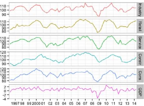
In Figure 1 the confidence indicators for the five sectors and the GDP quarter on quarter growth series is presented. From viewing Figure 1 it is clear that the confidence indicators reflects the movements in GDP and as such can be used for prediction.

(8)

2 DATA 7

Figure 1: Panel of confidence indicator variables and GDP. Confidence indica-tors are standardized with mean 100 and standard deviation 10. GDP series is the quarter on quarter growth rate.

Data for some of the predictor variables as well as GDP is available from as far back as the 1960s and 70s until today. However, in order to avoid missing values and large scale imputations we have restricted the observations to the second quarter of 1996 to the second quarter of 2014. This leaves 73 observations in total.

(9)

3 THEORETICAL MODELS 8

3 Theoretical Models

In order to investigate if the RF approach can bring forecast improvements to economics we first need to provide a brief overlook of the theoretical framework. We first give a brief account of the econometric method that is often used, which we use for evaluation. We then proceed by describing the RF algorithm in a stylized manner for easier comprehension.

3.1 Autoregressive Process

Often when evaluating econometric models we use simple linear models as benchmarks. According to Marcellino (2008) the simplest linear time series models are still, in a time when more sophisticated models are abundant, jus-tified and perform well when tested against alternative models, as long as they are well specified. The autoregressive process (AR) of order p is such a simple time series model which can be written as

Yt= p

X

i=1

φiYt−i+ ut, (1)

where φ1, ..., φp are constants and ut is a Gaussian white noise term. The

key assumption in this model is that the value of Yt−i can explain the behavior

of Y in time t. For this model to be stationary the relationship |φi| < 1 must

be fulfilled for all φi, otherwise the series will explode as t increases.

This type of model is frequently used in time series analysis and will therefore serve as our benchmark model for evaluating the performance of the RF. For more on the properties of the AR(p) process, see Asteriou and Hall (2011).

3.2 Example: Tooth Growth in Guinea Pigs

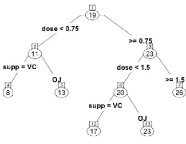
The RF method is based on regression trees and to illustrate how regression trees work we begin with an example. We have a dataset provided with R from C. I. Bliss (1952). It consists of observations on the tooth length (in mm) of 10 guinea pigs at three different dose levels of vitamin C (0.5, 1 and 2 mg) as well as two different methods of distribution, orange juice (OJ) and ascorbic acid (VC). The reason we can make different observations on the same guinea pigs is that their teeth are worn down when eating and as a result grow continuously. We fit the data to a regression tree with tooth length as the response variable and dosage and delivery method as predictor variables. In Figure 2 we find the regression tree diagram.

(10)

Figure 2: Tree diagram of fitted regression tree on guinea pig tooth data.

At each node in Figure 2 we have the splitting criterion. Observations that satisfy the criterion go to the left and those that do not go to the right. We get the node number on top and in the elliptical figure we have the average predicted tooth length of the observations that fall into that node. The node number corresponds to an output table provided by R and a sample of this is found in Table 2. To illustrate, the interpretation for node number 5 is is the following: the predicted tooth length of a guinea pig on a vitamin C dose less than 0.75 mg in form of orange juice is 13.23 mm with a MSE of 17.900.

Node Number Observations Mean Prediction MSE .. . ... ... ... 4 10 7.98 6.790 5 10 13.23 17.900 6 20 19.735 18.521 .. . ... ... ...

Table 2: Regression tree output table.

3.3 An Introduction to Random Forests

The RF was introduced by Breiman (2001a) and was an extension from his previous work on bagging (Breiman, 1996). It is an algorithm that can handle both high-dimension classification as well as regression. This has made it one

(11)

of the most popular methods in data mining. The method is widely used in different fields, such as biostatistics and finance, although it has not been applied to any greater extent in the field of economics. The algorithm itself is still to some extent unknown from a mathematical viewpoint and only stylized outlines are presented in textbooks and articles (Biau and D’Elia, 2011). Work is ongoing to map the algorithm but most papers focus on just parts at a time. The outlining of the RF method in this section draws heavily from Zhang and Ma (2012) and the chapter on RFs by Adele Cutler, D. Richard Cutler, and John R. Stevensand. The notation used by them is reproduced here.

3.4 A Forest Made of Trees

As the name itself suggests, the RF is a tree-based ensemble method where all trees depend on a collection of random variables. That is, the forest is grown from many regression trees put together, forming an ensemble. We can formally describe this as a p-dimensional random vector X = (X1, X2, ..., Xp)T

repre-senting the real-valued predictor variables and Y reprerepre-senting the real-valued response variable. Their joint distribution PXY(X, Y ) is assumed unknown.

This is one advantage of the RF, we do not need to assume any distribution for our variables. The aim of the method is to find a prediction function f (X) to predict Y . This is done by calculating the conditional expectation

f (x) = E(Y |X = x), (2)

known as the regression function. Generally ensemble methods construct f as a collection of ”base learners” h1(x), h2(x), ..., hJ(x) which are combined into

the ”ensemble predictor”

f (x) = 1 J J X j=1 hj(x). (3)

In the RF the jth base learner is a regression tree which we denote hj(X, Θj),

where Θj is a collection of random variables and for j = 1, 2, ..., J , these are

independent.

In RFs the trees are based on binary recursive partitioning trees. They partition the predictor space in a sequence of binary partitions or ”splits” on individual variables which form the branches of the tree. The ”root” node in the tree is made up of the entire predictor space. Nodes that are not split are called ”terminal nodes” or ”leaves” and these form the final partition of the predictor space. Each nonterminal node is split into two descendant nodes, one to the left and one to the right. This is done according to the value of one of the predictor variables based on a splitting criterion, called a ”split point”. Observations of the predictor variables smaller than the split point goes to the left and the rest to the right.

The split of a tree is chosen by considering every possible split on every predictor variable and then selecting the ”best” according to some splitting

(12)

criterion. If the response values at the nodes are y1, y2, ..., yn then a common

splitting criterion is the mean squared residual at the node

Q = 1 n n X i=1 (yi− ¯y)2 (4)

where ¯y is the average predicted value at the node. The splitting criterion provides a ”goodness of fit” measure with large values representing poor fit and vice versa. A possible split creates two descendant nodes, one on the left and one on the right. If we denote the splitting criterion for the possible descendants by QL and QR along with their respective sample sizes nL and nR, then the

split is chosen to minimize

Qsplit= nLQL+ nRQR. (5)

Finding the best possible split means sorting the values of the predictor vari-able and then considering every distinct pair of values. Once the best possible split is found the data is partitioned into the two descendants nodes which are in turn split in the same way as the original node. This procedure is recursive and stops when a stopping criterion is met. This can for example be that a specified number of unsplit nodes should remain. The unsplit nodes remaining when the stopping criterion is met are the terminal nodes. A predicted value for the respons variable is then obtained as the average value from the terminal nodes for all observations.

3.5 The Random Forest

Up until now we have the theoretical workings of one regression tree. Now we can begin to understand the RF. As mentioned before the RF will use base learners hj(X, Θj) as trees. We define a training setD = {(x1, y1), (x2, y2), ..., (xN, yN)}

in which xi= (xi,1, xi,2, ..., xi,p)T denotes the p predictor variables and yiis the

response, and a specific realization θj of the randomness component Θj, the

fitted tree is denoted ˆhj(x, θj,D). This is the original formulation by Breiman

(2001a) but we do not consider θj directly but rather implicitly as we inject

randomness into the forest in two ways. First of all every tree is fitted to an independent bootstrap sample of the original dataset. This is the first part of the randomness. The second part comes from splitting the nodes. Instead of each split being considered over all p predictor variables we use a random subset of m predictors. This means that different randomly assigned predictor variables are included in different trees.

When drawing the bootstrap sampleDjof size N from the training set some

observations are left out and do not make it into the sample. This is called ”out-of-bag data” and is used to estimate generalization errors (to avoid overfitting) and the variable importance measure described in section 3.7.

(13)

3.6 Tuning

Generally the RF is not sensitive and requires little to no tuning unlike other ensemble methods. There are three parameters that can tuned to improve performance if necessary. These are:

• m, the number of randomly assigned predictor variables at each node • J , the number of trees grown in the forest

• tree size, measured e.g. by the maximum number of terminal nodes The only parameter that seems to be sensitive in using RFs is m, the number of predictors at each node. When using RFs for regression m is chosen as m = p/3 where p is the total number of predictor variables (Zhang and Ma, 2012, p. 167). The potential problem that requires tuning is overfitting but as Diaz-Uriatre and Alvarez de Andres (2006) found, the effects of overfitting are small. Many ensemble methods tend to overfit when J becomes large. As Breiman (2001a) shows this is almost a non-issue with RFs; the number of trees can be large without consequence. Breiman (2001a) showes that the generalization error almost converges when J is grown beyond a certain number and so the only problem is that J not should be too small.

3.7 Variable Importance

When dealing with regression with many dimensions we can use principal com-ponents analysis to reduce the number of variables to include. The RF has its own method for determining which predictors are the most important to include. For example, to measure the importance of variable k, first the observation on the variable is passed down the tree and the predictions are computed. Then the values of k are randomly permuted in the out-of-bag data while keeping all other predictors fixed. Next the modified out-of-bag data are passed down the tree and a new set of predictions are computed. Using these two sets of data, the real set and the one based on the permutations, the difference in the MSE of the predictions from the two sets is obtained. The higher this number is, the more important the variable is deemed to be for the response.

3.8 Software

When estimating the RF and calculating the variable importance measure we use the open source statistical software R. The code produced in order to obtain our results is included in the appendix.

(14)

4 EMPIRICAL FINDINGS 13

4 Empirical Findings

Before we can estimate our benchmark model and the RF we must establish that the benchmark will perform well. In order to have the best possible model for comparison, the time series it is based on must be stationary and its process specified correctly. In the interest of a fair comparison we begin this section by investigating the GDP time series which we aim to predict.

4.1 Stationarity

The definition of a stationary process is a stochastic process that has a joint probability distribution that does not change over time. That means that if a process is stationary its mean and variance is also constant over time. This can be described as the process being in statistical equilibrium. The assumption of stationarity is important in order to make statistical inference based on the observed record of the process (Cryer and Chan, 2008).

To find out whether the quarter on quarter GDP series is stationary we formally test it using the Augmented Dickey-Fuller (ADF) test. The ADF-test tests for a unit root in the time series sample and the alternative hypothesis states that the series is stationary. When choosing the lag length for the test we use the Bayesian information criteria (BIC). The result of the ADF-test proves to be significant and is presented in Table 3. This means that the null hypothesis of a unit root is rejected at the one percent significance level and we thus conclude that the series is stationary. When choosing lag length using other criterions such as the Akaike information criteria (AIC) we arrive at the same result. We therefore conclude that it is more or less arbitrary which information criterion we use and choose to present only the result where BIC is used.

Variable t statistic p-value

GDP Growth Series −3.300 < 0.01

Note. Lag length for the ADF test is based on the Bayesian information criterion.

Table 3: Unit root test.

4.2 Autocorrelation

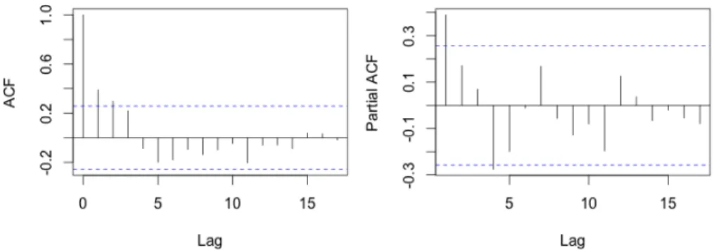
In order to best estimate and forecast the GDP growth series we investigate the correlograms for the autocorrelation function (ACF) and the partial autocorre-lation function (PACF). These are featured in Figure 3.

(15)

Figure 3: Correlogram φ = 0.381.

In the correlogram of the ACF we notice the rapidly decreasing pattern in the spikes which indicates an autoregressive process with short memory. In the correlogram of the PACF we have one significant spike at the first lag. When we weight these two results together we arrive at the conclusion that the observed process is an AR of order one.

4.3 AR(1)

After having examined the properties of the GDP growth series, we are now ready to estimate the benchmark model. We begin by partitioning our dataset into two parts. One training set which we use for building the model and one test set over which we evaluate by forecasting. The training set consists of the observations from the second quarter of 1996 to the third quarter of 2010. The test set thus contains observations from the fourth quarter of 2010 to the second quarter of 2014. We have chosen to divide the dataset this way to have approximately 80 percent of the observations in the training set and 20 percent in the test set. We fit an AR(1) with a drift component to the GDP growth series to the training set.

The output produced shows the φ-coefficient to be 0.381 which is reflected in the ACF correlogram. When the model is fitted we can use what it has learned to forecast over our test set. We use the built in prediction function available in R and arrive at an RMSE of 0.949 for the benchmark model. This value is interpreted, compared and further elaborated on in Table 7 in section 4.6.

4.4 Random Forest

The RF approach is very well suited to address this kind of estimation. We have a high dimensional regression problem (n << p) since we have 58 observations in the training set and p = 466 predictor variables to choose from.

(16)

We begin by partitioning the dataset in the same way as for the AR estima-tion. We estimate the model with J = 500 trees and the algorithm randomly selects m = 155 predictor variables to compare at each node split instead of the p = 466 available. We are given an R2 of 27.96 percent. This means that approximately 28 percent of the variation in quarterly GDP growth rate is explained by the variables included in the model. Table 4 lists the ten most important predictors as decided by the algorithm.

Variable Mean Decrease

Consumer 3 alt. 2 Sm− Sm−3 3.735 Retail 1 alt. 3 3.320 Cof retail 3.288 Industry 4 alt.1 3.182 Consumer 3 alt.6 Sm− Sm−1 3.010 Consumer 4 alt.4 2.990 Consumer 10 alt.1 Sm− Sm−1 2.825 Retail 3 2.725 Consumer 6 2.650 Industry 6 alt.3 2.441

Note. All questions and alternatives are fully outlined in the appendix.

Table 4: Variable importance table.

The predictors listed in Table 4 are calculated as described in section 3.7. The mean decrease is the mean decrease in prediction accuracy as measured by the MSE if the predictor was to be removed from the model. The most important predictor for the quarterly GDP growth rate according to the RF algorithm is a difference series of consumer question three, alternative two. This question regards consumers and reads ”[h]ow do you think the general economic situation in the country has changed over the past 12 months?” and the second alternative is ”got a little better”. All questions and alternatives are fully outlined in the appendix. When examining the whole output displaying the relevance of the predictor variables we note that the difference between one variable and the next in the ranking, decreases rapidly after the tenth variable. It could therefore be hard to motivate where to draw the line for how many variables to include after this point. This is why we choose to include the ten most relevant variables.

Again we use the model built to forecast the GDP growth rate over the test set. The RMSE is 0.753 for the RF model. This value is interpreted, compared and further elaborated on in Table 7 in section 4.6.

(17)

4.5 Ad Hoc Linear Model

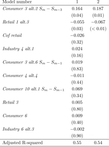
We have used the RF approach to find the key variables explaining GDP growth rate in our dataset. We now wish to estimate a linear model containing these variables and use it to make a prediction of GDP growth rate. To this end we use the same partitioning as previously where the training set consists of approximately 80 percent of the observations and the test set consists of 20 per-cent of the observations. Estimation of the model is done in two steps. Firstly, we estimate the model using the ten variables ranked as the most important in explaining GDP by the RF. Secondly, we choose those variables that showed to be significant and estimate the reduced model. The result of this procedure can be seen in Table 5 where we present the coefficients and p-values for each variable in the two models.

Model number 1 2 Consumer 3 alt.2 Sm− Sm−3 0.164 0.187 (0.04) (0.01) Retail 1 alt.3 −0.055 −0.067 (0.03) (< 0.01) Cof retail −0.026 (0.32) Industry 4 alt.1 0.024 (0.16) Consumer 3 alt.6 Sm− Sm−1 0.019 (0.83) Consumer 4 alt.4 −0.011 (0.44) Consumer 10 alt.1 Sm− Sm−1 0.069 (0.34) Retail 3 0.005 (0.80) Consumer 6 0.009 (0.40) Industry 6 alt.3 −0.002 (0.90) Adjusted R-squared 0.55 0.54

Note. P -values in brackets.

Table 5: First and final ad hoc linear model.

In the second estimation there are only two variables remaining, which proved to be significant in the first model. These are denoted ”Consumer 3

(18)

alt.2 Sm− Sm− Sm−3 and ”Retail 1 alt.3”. The first question regards

con-sumers and reads ”[h]ow do you think the general economic situation in the country has changed over the past 12 months?” and the second alternative is ”got a little better”. Looking at Table 5 we note that this variable has a pos-itive influence on GDP growth. This is plausible given that consumers being optimistic about the economic situation should naturally influence it positively. The second question regards the retail sector and reads as follows: ”[h]ow has (have) your business activity (sales) developed over the past three months?”, response option 3 being ”deteriorated (decreased)”. This variable naturally has a negative effect on GDP growth which can also be seen in Table 5. When using this model to forecast we arrive at an RMSE of 0.790. This value is interpreted, compared and further elaborated on in Table 7 in section 4.6.

It should be mentioned that we have not performed any diagnostic tests on the model since the main purpose of this study is to compare the forecasts between the AR(1) and RF. The linear model should thus be interpreted with caution.

4.6 Evaluation

To evaluate our three different ways of forecasting the quarterly GDP growth rate we have gathered the predicted and observed values in Table 6. The dif-ference between the RF and ad hoc linear model is marginal but the AR(1) estimates larger differences. When we compare observed to predicted values the RF performs best closely followed by the linear model, but the AR(1) performs poorly.

(19)

Forecast Observed Difference

AR(1) RF RF LM GDP qoq AR(1) RF LM

2010Q4 0.9 1.0 1.0 1.7 0.8 0.7 0.7 2011Q1 1.2 1.1 0.4 0.1 1.1 1.0 0.3 2011Q2 0.5 0.8 0.5 0.2 0.3 0.6 0.3 2011Q3 0.6 0.1 −0.3 1.0 0.4 0.9 1.3 2011Q4 0.9 0.2 −0.8 −1.7 2.6 1.9 0.9 2012Q1 −0.2 0.6 0.7 0.5 0.7 0.1 0.2 2012Q2 0.7 0.6 0.0 0.6 0.1 0.0 0.6 2012Q3 0.7 0.4 −0.6 0.0 0.7 0.4 0.6 2012Q4 0.5 0.2 −0.4 −0.4 0.9 0.6 0.0 2013Q1 0.3 0.6 −0.8 1.2 0.9 0.6 2.0 2013Q2 0.9 0.5 0.1 −0.4 1.1 0.9 0.5 2013Q3 0.4 0.7 0.9 1.2 0.1 0.5 0.3 2013Q4 0.7 0.7 0.8 −0.2 0.5 0.9 1.0 2014Q1 0.9 1.0 1.1 0.1 0.8 0.9 1.0 2014Q2 0.5 0.7 1.2 0.7 0.2 0.0 0.5 Sum 11.2 9.9 10.1

Table 6: Forecasted values divided by model and observed quarterly GDP growth rate.

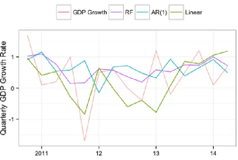
In Figure 4 the predicted values of the AR(1), the RF and the linear model are plotted together. We notice that the all three models try to capture the movements of the GDP growth series.

(20)

Figure 4: Observed quarterly GDP growth rate plotted against predicted values of the AR(1), the RF and the linear model.

To compare the forecasting errors between the different models we use the root mean squared errors (RMSE) as a measure of accuracy. The mean squared error (MSE) is a measure of the average squares of the errors. In other words it measures the difference between the estimated values and the observed values. The RMSE is simply the square root of the MSE which can be easier to interpret since it has the same units as the quantity being estimated, i.e. the GDP growth rate.

Model RMSE

Present study Biau and D’Elia

AR(1) 0.949 0.8

Random Forest 0.753 0.66

Linear Model 0.790 0.37

Table 7: Root mean square errors.

The RMSEs of the three models are presented in Table 7. The difference between the RF and the linear model is small although the RF model performs considerably better than the AR(1). The RMSE based on the forecasts of the

(21)

RF model is 0.753 i.e. the average error in forecasting quarterly GDP growth rate is approximately 0.75 percentage points.

Biau and D’Elia (2011) found that the linear model based on the predictors chosen by the RF performed best when forecasting GDP growth in the Euro area. Their estimates are found in Table 7 alongside those found in this study. Biau and D’Elia (2011) also found that the AR forecast gave the poorest perfor-mance. They estimated the RMSE for their RF model to 0.66 and the RMSE for their linear model to 0.37. This differs from our results in that their linear model showed the best performance as opposed to the present study where the linear model did not perform better than the RF. We could possibly have arrived at a different result if we had used other predictors in the first estimation of the linear model. Another explanation for their RMSEs overall being lower than ours may be that the corresponding quarterly GDP growth series for the Euro area which they analyze is smoother than the Swedish dito (Taborda, Trading Economics, 2014). The smoother series is easier for the models to forecast.

As previously stated the RMSE for the RF model in the present study is estimated to 0.753. This is the smallest error and thus the RF model performs better than the benchmark, supporting our theory that there are benefits to using data mining techniques on economic time series. There is nonetheless only a slight difference between the ad hoc linear model predictions and those made using the RF. When forecasting using the RF approach the model was not helped by the massive amount of data provided. The ad hoc linear model performs almost as well as the RF. This result highlights the use of the RF algo-rithms variable importance measure. Using a combination of the two methods can be argued for, depending on what results are needed. If the magnitude of influential variables are desired this is a recommended approach.

The AR(1) model estimated with a drift component captures the movements of the GDP growth series with a lag and predicts values further from the ob-served than the RF. In this study the difference in performance between the RF and the benchmark is noticeable. We believe that the differences and benefits of more data driven, complex models such as the RF would be emphasized to a greater extent if the target response variable did not show any clear patterns of a known process. This would benefit the RF and make better use of its ca-pabilities.

The result of this study would suggest that economic forecasts can be im-proved by using RFs. Whether or not this is the case future research will prove but regardless it can be problematic to use these kind of ”black-box” models to model economics. The reason for making any forecasts is to make decisions, and in doing so we need as much information as possible. When using the RF we are not made privy to the influences of the input variables. This means we may make better predictions for certain response variables but at the expense of not knowing what affects them in what way.

(22)

5 CONCLUSION 21

5 Conclusion

GDP can be used as a measure of the economic state of a country. It is there-fore important in order to make policy decisions concerning the economy. The purpose of this study is to investigate possible forecasting improvements in the quarterly GDP growth rate using the data mining technique Random Forests developed by Breiman (2001a). It has previously enjoyed good prediction re-sults in other fields of study but has not yet broken through to the economic society.

Using a dataset with 466 time series built on the Economic Tendency Survey conducted by the National Institute of Economic Research in Sweden, including e.g. confidence indicators, we have estimated a benchmark AR(1) with a drift component, a Random Forest and an ad hoc linear model based on influential predictors chosen by the Random Forest algorithm. The models were estimated on a training set and evaluated by forecasting over a test set corresponding to an 80/20 split.

We have used the RMSE to evaluate the model performance when fore-casting. The Random Forest proved marginally better than the ad hoc linear model and both are noticeably better than the benchmark AR(1) with RMSEs of 0.753, 0.790 and 0.949 respectively. Before any general conclusions can be drawn this result should be verified in other studies. Nonetheless it supports the hypothesis that Random Forests can bring forecasting improvements when applied to economic data; either as a means to building a well performing linear model or by itself.

Future research should include more data, e.g. economic ”hard” variables, in estimation and continue to explore data driven techniques in economics.

(23)

6 REFERENCES 22

6 References

Asteriou, D. and Hall, S. G., (2011). ”Applied Econometrics,” 2nd edition, Pal-grave MacMillan

Benito Garzon, M., Sanchez de Dios, R. and Sainz Ollero, H., (2008), ”Ef-fects of climate change on the distribution of Iberian tree species”. Applied Vegetation Science, 11, pp. 169-178.

Biau, O. and D’Elia, A., (2011), ”Euro area GDP forecasting using large survey datasets”.

Breiman, L., (2001a). ”Random Forests”, Machine Learning 45 (1) pp. 5-32.

Breiman, L., (2001b). ”Statistical Modeling: The Two Cultures (with com-ments and a rejoinder by the author)”. Statistical Science 16, no. 3, pp. 199-231.

Breiman, L., (1996). ”Bagging Predictors”, Machine Learning 24 (2) pp. 123-140.

C. I. Bliss, (1952), ”The Statistics of Bioassay”. Academic Press.

Cryer, J.D. and Chan, K., (2008). ”Time series analysis: with applications in R”, Springer, New York.

Diaz-Uriarte, R., Alvarez de Andres, S., (2006). ”Gene Selection and Classi-fication of Microarray Data Using Random Forest”, BMC Bioinformatics 7 (1) 3.

Gutirrez, N. L., Hilborn, R., and Defeo, O., (2011). ”Leadership, social capi-tal and incentives promote successful fisheries”, Nature, 470(7334), pp. 386-389.

Kenny, C. and Williams, D., (2001). ”What do we know about economic growth? or, why don’t we know very much?”. World development, 29(1), 1-22.

Marcellino, M., (2008). ”A linear benchmark for forecasting GDP growth and inflation?”, Journal of Forecasting 27.4, pp. 305-340.

Taborda, J., (2014). ”Euro Area GDP Growth Rate”, Trading Economics, Available from: http://www.tradingeconomics.com/euro-area/gdp-growth [4 De-cember 2014]

Adele Cutler, D. Richard Cutler, John R. Stevensand, (2012). ”Random Forets” in Zhang, C. and Ma, Y. [Eds.], ”Ensemble Machine Learning: Meth-ods and Applications”, pp. 157-177, Springer Science Business Media

(24)

7 APPENDIX 23

7 Appendix

7.1 R Code

#Verify AR pattern acf(train$gdp_qoq) pacf(train$gdp_qoq) #ADF test library(urca)

df <- ur.df(train$gdp_qoq, type="drift", lags=1 , selectlags="BIC")

summary(df)

#Estimating the AR(1) library(forecast)

gdp.ar <- Arima(train$gdp_qoq, order=c(1,0,0), include.drift=TRUE) #Specifying the ARIMA(1,0,0)

#Forecast

pred.ar <- gdp.ar

pred2.ar <- Arima(test$gdp_qoq, model=pred.ar) onestep <- fitted(pred2.ar)

onestep

#RMSE

library(Metrics)

rmse(test$gdp_qoq, onestep)

#The Random Forest

dim(train) #Get dimensions of data frame

train[1:58, 2:470] <- sapply(train[1:58, 2:470],

as.numeric) #Convert all predictors to numeric variables

set.seed(131) #Set randomizing seed for replication study

#The Random Forest Algorithm library(randomForest)

gdp.rf <- randomForest(gdp_qoq ~ . -date -gdp -gdp_qoq -gdp_index, data=train, importance=TRUE)

print(gdp.rf)

#Variable importance measure

imp <- importance(gdp.rf, type = 1) round(imp, 3)

(25)

7 APPENDIX 24

#Prediction dim(test)

test[1:15, 2:470] <- sapply(test[1:15, 2:470], as.numeric) pred.rf <- predict(gdp.rf, newdata=test, n.ahead=15) pred.rf

#RMSE

rmse(test$gdp_qoq, pred.rf)

#Ad Hoc Linear model library(stats)

fit <- lm(gdp_qoq ~ consumer_3_alt.2_t.3.1 + retail_1_alt.3 + cof_retail + industry_4_alt.1 + consumer_3_alt.6_t.1 + consumer_4_alt.4 + consumer_10_alt.1_t.1 + retail_3 + consumer_6 + industry_6_alt.3, data=train)

#Estimating first model summary(fit)

fit2 <- lm(gdp_qoq ~ consumer_3_alt.2_t.3.1 + retail_1_alt.3 , data=train)

#Estimating final model summary(fit2)

#Forecast

lm.pred <- predict(fit2, newdata=test, n.ahead=15) lm.pred

#RMSE

(26)

7 APPENDIX 25

7.2 Survey Questionnaire

7.2.1 Industry quarterly questions

Q1 How has your production de-veloped over the past three months? it has...

1. increased

2. remained unchanged

3. decreased

Q2 How do you assess your current production capacity? The current pro-duction capacity is...

1. more than sufficient

2. sufficient

3. not sufficient

Q3 At what capacity is your com-pany currently operating (as percent-age of full capacity)?

The company is currently operat-ing at...% of full capacity.

Q4 How have your orders devel-oped over the past three months?

1. increased

3. decreased

Q5 How do you assess your cur-rent total order books? They are (rel-atively)..

2. sufficient

3. not sufficient

Q6 How do you assess your current export order books? They are (rela-tively)...

2. sufficient

3. not sufficient

Q7 How has your competitive posi-tion on the domestic market developed over the past 3 months? It has...

1. improved

3. deteriorated

Q8 How has your competitive posi-tion on the foreign markets inside EU developed over the past 3 months? It has...

1. improved

3. deteriorated

Q9 How has your competitive posi-tion on the foreign markets outside EU developed over the past 3 months? It has...

1. improved

(27)

7 APPENDIX 26

Q10 Do you consider your current stock of finished products to be...?

1. too large

2. adequate

3. too small

Q11 How do you expect your pro-duction to develop over the next three months? It will...

1. increase

2. remain unchanged

3. decrease

Q12 How do you expect your ex-port orders to develop over the next three months? They will...

1. increase

2. remain unchanged

3. decrease

Q13 How do you expect your firm’s total employment to develop over the next three months? It will...

1. increase

2. remain unchanged

3. decrease

7.2.2 Retail quarterly questions

Q1 How has your business activity (sales) developed over the past three months? (Compared to the same pe-riod last year)

1. increased

3. decreased

Q2 How do you consider the vol-ume of the stock you currently hold to be?

1. too large

2. adequate

3. too small

Q3 How do you expect your busi-ness activity (sales) to change over the next three months? (Compared to the same period last year)

1. increase

2. remain unchanged

3. decrease

Q4 How do you expect your orders placed with suppliers to change over the next three months? (Compared to the same period last year)

1. increase

2. remain unchanged

3. decrease

Q5 How do you expect your firm’s total employment to change over the next three months? (Compared to the same period last year)

1. increase

2. remain unchanged

(28)

7 APPENDIX 27

7.2.3 Consumers monthly questions

Q1 How is the financial situation of your household compared to 12 months ago? 1. a lot better 2. a little better 3. the same 4. a little worse 5. a lot worse 6. do not know

Q2 How do you expect the finan-cial situation of your household to be 12 months from now?

1. a lot better 2. a little better 3. the same 4. a little worse 5. a lot worse 6. do not know

Q3 How do you think the general economic situation of the country is compared to 12 months ago?

Q4 How do you expect the general economic situation of the country to be 12 months from now?

Q5 How do you expect the number of unemployed people in this country to change over the next 12 months?

1. increase sharply

2. increase slightly

3. remain the same

4. fall slightly

5. fall sharply

6. do not know

Q6 In view of the general economic situation, do you think that now is the right moment for people to make ma-jor purchases such as furniture, electri-cal/electronic devices, etc.?

1. yes, it is the right moment now

2. not used in this question

3. it is neither the right nor the wrong moment

5. no, it is not the right moment

(29)

7 APPENDIX 28

Q7 Compared to the past 12 months, do you expect your house-hold to spend more or less money on major purchases (furniture, electri-cal/electronic devices, etc.) over the next 12 months?

1. much more

2. a little more

3. about the same

4. a little less

5. much less

6. do not know

Q8 In view of the general economic situation, do you think that now is the right moment to save? (Saving also in-cludes paying back on a loan)

1. yes, it is a very good moment to save

2. yes, it is a fairly good moment to save

3. it is neither a good nor a bad mo-ment to save

4. no, it is not a good moment to save

5. no, it is a very bad moment to save

6. do not know

Q9 How likely is your household to save money over the next 12 months? (Saving also includes paying back on a loan)

1. very likely

2. fairly likely

4. not likely

5. not likely at all

6. do not know

Q10 Which of these statements best describes your household’s current financial situation?

1. we are saving a lot

2. we are saving a little

3. we are just managing to make ends meet on income

4. we have to draw on our savings/ running into debt to some extent

5. we have to draw on our savings/ running into debt to a large ex-tent

6. do not know

Q11 How likely is your household to buy a car over the next 12 months?

1. very likely

2. fairly likely

4. not likely

6. do not know

Q12 Is your household planning to buy or build a home over the next 12 months (to live in permanently, as a holiday house or to let?

1. yes, definitely

2. possibly

4. probably not

5. no

(30)

7 APPENDIX 29

Q13 How likely is your household to spend any large sums of money on home improvements or renovations over the next 12 months (on permanent home or holiday house)?

1. very likely

2. fairly likely

4. not likely

6. do not know

7.2.4 Confidence indicators

Industry: Current total order books (Q5)− current stock of finished products (Q10) + expected production volume (Q11)

Retail: Sales volume, turn-out (Q1) − current volume of stock (Q2) + expected sales volume (Q3)

Services: Business development, turn-out + demand for the firm’s services, turn-out + expected demand for the firm’s services

Construction: Current order books + expected numbers of employees

Consumers: Is calculated as an average of the net balance of positive and negative answers to the questions Q1, Q2, Q3 and Q4 (consumers monthly questions).

Forecasting GDP Growth, or How Can Random Forests Improve Predictions in Economics?

Bachelor Thesis

Statistics