ANALYSIS OF STRESS AND GEOMECHANICAL PROPERTIES IN THE NIOBRARA FORMATION OF WATTENBERG FIELD,
COLORADO, USA
by
c
Copyright by Alexandra K. Grazulis, 2016 All Rights Reserved
A thesis submitted to the Faculty and the Board of Trustees of the Colorado School of Mines in partial fulfillment of the requirements for the degree of Master of Science (Geo-physics). Golden, Colorado Date Signed: Alexandra K. Grazulis Signed: Dr. Thomas L. Davis Thesis Advisor Golden, Colorado Date Signed: Dr. Terence K. Young Professor and Head Department of Geophysics
ABSTRACT
In Wattenberg Field the Niobrara Formation is the primary productive zone for horizontal drilling and completions. It is an unconventional reservoir made up of alternating chalk and marl layers which require hydraulic fracturing for completion. The main study area for this project is a four square mile region where time-lapse multicomponent seismic surveys have been acquired. This area includes the Wishbone section, where 11 horizontal wells have been drilled, and is the focus of dynamic reservoir characterization. The primary goal of this research study is to investigate relationships between geomechanics, stress and fractures. Determining the geomechanical properties of the reservoir is essential for better reservoir management.
Geology is the main driver controlling production, due to the presence of fault compart-mentalization in the field. The central graben, within the Wishbone section, causes geologic heterogeneity and displays signs of high net pressure. This is due to a larger increase in pore pressure, ultimately decreasing effective stress. Outside of the graben, naturally fractured areas, displaying decreasing net pressure trends, will maximize fracture network surface area during completions. This allows for a larger volume of rock to be stimulated, and a greater chance of opening pre-existing fractures. As far as re-fracturing efforts are concerned, areas outside of the graben which are brittle and have low stress anisotropy should be targeted to create complex fracture networks.
Geomechanical and stress information about the reservoir is vital for predicting fracture propagation. After investigation of fracture characterization trends, we have a better under-standing of stimulated areas within the Wishbone section. Specific completion techniques can be applied to stages based on geomechanical properties and geologic location. Fracture networks defined through the integrated dynamic reservoir characterization process provide targets for future re-fracturing efforts.
TABLE OF CONTENTS
ABSTRACT . . . iii
LIST OF FIGURES AND TABLES . . . vii
LIST OF SYMBOLS . . . x LIST OF ABBREVIATIONS . . . xi ACKNOWLEDGMENTS . . . xii DEDICATION . . . xiii CHAPTER 1 INTRODUCTION . . . 1 1.1 Motivation . . . 1 1.2 Field Background . . . 2 1.3 Geologic History . . . 5 1.4 Stress History . . . 9 1.5 Methodology . . . 11 1.5.1 Data Inventory . . . 12 1.5.2 Stress Analysis . . . 12 1.5.3 Structural Modeling . . . 13 1.5.4 Simulations . . . 13
1.5.5 Analysis and Recommendations . . . 13
CHAPTER 2 LITERATURE REVIEW . . . 15
2.1 Geomechanics in Unconventional Reservoirs . . . 15
2.3 Role of Geomechanics in Hydraulic Fracturing . . . 22
2.4 Stress Shadow Effect . . . 23
CHAPTER 3 STRESS ANALYSIS . . . 25
3.1 Completion Reports . . . 25
3.2 Net Pressure Trends . . . 27
CHAPTER 4 MODELING PROCESS . . . 33
4.1 Data Collection and Well Normalization . . . 33
4.2 Structural Model . . . 34 4.2.1 Wells . . . 36 4.2.2 Core . . . 38 4.2.3 Seismic . . . 40 4.2.4 Model . . . 40 4.3 Integration of RCP Work . . . 40 4.4 Preliminary Interpretations . . . 42
CHAPTER 5 GEOMECHANICAL SIMULATIONS . . . 49
5.1 Simulation Process . . . 49
5.2 Stress Changes . . . 51
5.3 Moving Forward . . . 55
CHAPTER 6 COMPARISON DATA . . . 57
6.1 Microseismic . . . 57
6.2 Image Logs . . . 59
6.3 Rock Quality Index . . . 61
6.5 Shear Seismic . . . 64
CHAPTER 7 CONCLUSIONS AND RECOMMENDATIONS . . . 71
7.1 Future Work . . . 72
LIST OF FIGURES AND TABLES
Figure 1.1 Map of Wattenberg Field. . . 3
Figure 1.2 Wells of interest in Turkey Shoot. . . 5
Figure 1.3 Timeline of seismic acquisition and well development. . . 6
Figure 1.4 Map of seismic surveys. . . 7
Figure 1.5 Stratigraphic column of Wattenberg Field . . . 10
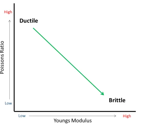
Figure 2.1 Young’s Modulus vs. Poisson’s Ratio. Arrow pointing in the direction of increasing brittleness for a fixed stress state. . . 17
Figure 2.2 Principal stresses acting on a normal fault, as described by the Anderson fault classification system. . . 19
Figure 2.3 Diagram of principal stresses for a vertical well. . . 20
Figure 2.4 Diagram of principal stresses for a horizontal well aligned with minimum horizontal stress. . . 21
Figure 2.5 Schematic of an initial and secondary fracture from a re-fracturing effort . . . 24
Figure 3.1 11 wells within the Wishbone section. . . 26
Figure 3.2 Example treatment plot. . . 26
Figure 3.3 Net pressure trends. . . 28
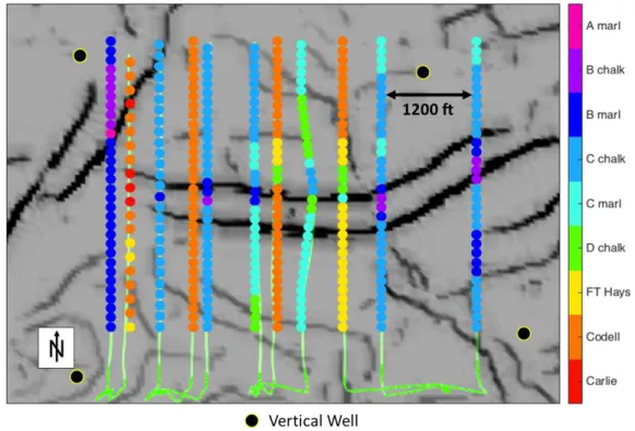
Figure 3.4 11 Wishbone wells with stages color coded by lithology. . . 29
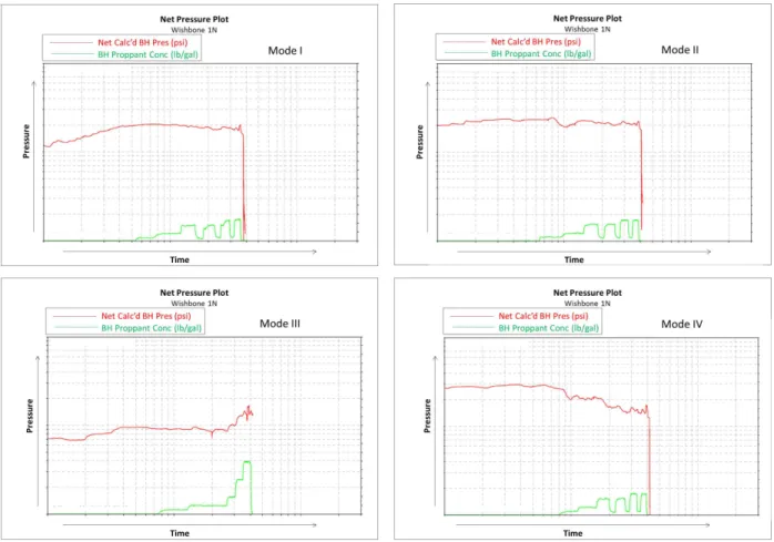
Figure 3.5 Net pressure plots from different stages for well 1N, each representing a different fracture characterization mode. . . 30
Figure 3.6 Stages for wells 1N, 2N, 6N, 7N and 9N color coded by net pressure trend mode. . . 31 Figure 3.7 Stages for wells 1N, 2N, 6N, 7N and 9N color coded by net pressure
Figure 4.1 Wells in existing project (blue). New wells added and normalized (red). . 35
Figure 4.2 Example histograms of well normalization for Gamma Ray log. . . 36
Figure 4.3 Structural modeling process. . . 37
Figure 4.4 Map displaying Core Well #3 in relation to the Wishbone section. . . 38
Figure 4.5 Core Well #3 logs. Black data points represent CCS values determined from core testing. . . 39
Figure 4.6 Top Niobrara structure map displaying locations of the wells (red) used in velocity model. . . 41
Figure 4.7 Final Turkey Shoot structural model; layers distinguihsed by color. . . 42
Figure 4.8 Poisson’s Ratio inversion volume - Top of C Chalk. . . 43
Figure 4.9 Cross section of Poisson’s Ratio inversion. . . 43
Figure 4.10 Cross section of geometrically modeled Poisson’s Ratio. . . 44
Figure 4.11 Cross section of Poisson’s Ratio inversion with wellbore locations. . . 45
Figure 4.12 Cross section of Young’s Modulus with wellbore locations. Young’s Modulus calculated using well logs. . . 45
Figure 4.13 Cross section along plane of well 1N. . . 46
Figure 4.14 CSS inversion volume - Top of C Chalk. . . 46
Figure 4.15 Cross section of the percent difference of Zp for the baseline survey subtracted from the monitor survey. . . 48
Figure 5.1 Reservoir Geomechanics workflow for Visage simulations. Workflow is modified from Schlumberger. . . 50
Figure 5.2 In-situ stresses within Wishbone. Maximum horizontal stress (red) and minimum horizontal stress (blue). . . 52
Figure 5.3 Qualitative pressure volume (slice = Top of C Chalk) for initial pressure and one year after production of well 6N. . . 53
Figure 5.4 Example of a possible simulation output showing horizontal stress magnitudes and azimuths at these same time-steps. . . 54
Figure 5.5 Image displaying a possible stress reversal region for one stage in well
6N. . . 56 Figure 6.1 Microseismic events, color coded by stage, for wells 1N, 2N, 6N, 7N and
9N. . . 58 Figure 6.2 Microseismic events, color coded by stage, for wells 1N, 2N, 6N, 7N and
9N. Top of Niobrara C Chalk slice through Poisson’s Ratio inversion
volume. . . 59 Figure 6.3 Open natural fractures interpreted for wells 2N and 6N . . . 60 Figure 6.4 Rose diagram of drilling induced fractures for well 6N . . . 61 Figure 6.5 Cross section through Poisson’s Ratio volume along plane of well 2N. . . 63 Figure 6.6 Tracer study design. . . 64 Figure 6.7 Percentage difference in monitor and baseline anisotropy volumes. . . 65 Figure 6.8 Stages representing net pressure Mode IV (blue) for wells 1N, 2N, 6N,
7N and 9N, overlain onto percentage difference anisotropy volume. . . 66 Figure 6.9 Stages representing net pressure Mode II (orange) for wells 1N, 2N, 6N,
7N and 9N, overlain onto percentage difference anisotropy volume. . . 67 Figure 6.10 Map of the 11 Wishbone wells. Niobrara producing wells are labeled
and color coded to match corresponding production curves in the
following figure. . . 69 Figure 6.11 Normalized production plot of Niobrara wells within Wishbone. . . 70 Table 1.1 Geophysical surveys . . . 6
LIST OF SYMBOLS
Stress . . . σ Maximum Principal Stress . . . σV Maximum Horizontal Stress . . . σH Minimum Horizontal Stress . . . σh Young’s Modulus . . . E Poisson’s Ratio . . . ν Bulk Density . . . ρ Compressional Velocity . . . Vp Shear Velocity . . . Vs Compressional Impedance . . . Zp Shear Impedance . . . Zs Tensile Strength . . . σT Hoop Stress . . . σ′ θH Pore Pressure . . . Pp Wellbore Pressure . . . Pw Gravitational Constant . . . g
LIST OF ABBREVIATIONS
Colorado School of Mines . . . CSM Reservoir Characterization Project . . . RCP Energy Information Agency . . . EIA Anadarko Petroleum Corporation . . . APC Stimulated Reservoir Volume . . . SRV Produced Reservoir Volume . . . PRV Three Dimensional . . . 3D Four Dimensional . . . 4D Time-Lapse . . . 4D True Vertical Depth . . . TVD Rock Quality Index . . . RQI Confined Compressive Strength . . . CCS Closure Stress Scalar . . . CSS Instantaneous Shut In Pressure . . . ISIP Enhanced Oil Recovery . . . EOR Barrel . . . bbl Barrel Oil Equivalent . . . BOE
ACKNOWLEDGMENTS
I would first like to thank my family for their amazing support throughout my time at Colorado School of Mines. They have always been my rock and without them none of this would have been possible.
I would like to acknowledge the Colorado School of Mines and the Geophysics Depart-ment for the opportunity to complete both my undergraduate and graduate degrees at this institution. The material learned on this campus has been invaluable and I know will allow me to be successful in my future endeavors. To the Reservoir Characterization Project and all who are involved, I feel so fortunate to have been able to be a part of this outstand-ing research group. I would like to thank Anadarko Petroleum Corporation for supplyoutstand-ing data and knowledge to RCP and dedicating their time to helping students throughout this project. To my advisor, Tom Davis, I am thankful for his dedication and support during my time at CSM. The completion of this thesis would not have been possible without him. To Tom Bratton, who has been an unending vault of knowledge and has contributed so much of his time to helping with this research. I truly appreciate his passion for working with students and the expertise he brings to this consortium. I would also like to thank my thesis committee members, Azra Tutuncu and Jeff Andrews-Hanna, for their support and guid-ance throughout my research. To Michelle Szobody and Sue Jackson, for their hard work keeping everyone on track, and always happy to answer any questions or concerns. Finally I would like to thank the students of RCP, who I am fortunate to now call close friends. Peer support is so important throughout this process and I am forever grateful for their help and compassion during my research.
CHAPTER 1 INTRODUCTION
The Reservoir Characterization Project, RCP, is an industry sponsored consortium which is currently conducting research on Wattenberg Field, Denver Basin, Colorado. The main focus is to integrate geophysics, geology and petroleum engineering to perform dynamic reservoir characterization on unconventional formations. This work focuses on creating a 3D geomechanical model to understand stress changes and heterogeneity throughout the Niobrara and Codell Formations.
1.1 Motivation
Within the last decade, the exploration and production of shale reservoirs has increased significantly, due to coupled horizontal drilling and hydraulic fracturing applications, along with other advancements in completion technologies. The demand for energy is continually increasing and with the decline of conventional reservoirs, the importance of understanding unconventional reservoirs is even greater. The Energy Information Agency (EIA) reports that continued growth in domestic production of crude oil from tight formations leads to a decline in net imports of crude oil and petroleum products. The EIA predicts that the net import share of crude oil and petroleum products supplied will drop from 33% to 17% by 2040. Unconventional production will play a critical role in meeting these EIA projections. Approximately 51% of the proven tight gas reserves in the lower 48 states are located in the Rocky Mountain region (McCallister, 2000). The Wattenberg Field will be one of the key unconventional reserve areas in the US in helping meet the EIA projections; and for moving toward future energy independence.
The Wattenberg Field is a tight oil and gas field, discovered in 1970. It is one of the largest basin-centered gas fields in the Rocky Mountain region, in terms of reserves, surface area, and
number of wells. The field is located at the intersection of the basin axis and the northeast-trending zone of high heat flow. The combination of this high heat flow and deep burial is the reason for the large amount of hydrocarbon generation within the field (Ladd, 2011). Targeted intervals include the Niobrara and Codell Formations. The Niobrara is formed from interbedded chalk and marl layers, and has very low porosity and permeability. The Codell is a sandstone of slightly higher permeability. The main source beds for the Niobrara and Codell are contained within the Niobrara. Vertical well production has been occurring since the 1970s, and horizontal drilling since the 2000s. Development has shifted among different productive formations over time due to new discoveries, prices, and technology advances, like hydraulic fracturing. Most new wells in Wattenberg are targeting the Niobrara and Codell Formations and are horizontal. Most wells are drilled north-south due to the stress field and in attempt to maximize number of wells per section. Throughout all of Wattenberg Field there is varying well spacing, length, and completion techniques used, which is based upon the stress orientation, fracture network and permeability of the area. The challenge in this field is how to combine geology and engineering to maximize production. The goal of this research project is to help understand the geomechanics and stress field changes of the Wattenberg to aid in drilling and completion design of the Niobrara and Codell Formations. 1.2 Field Background
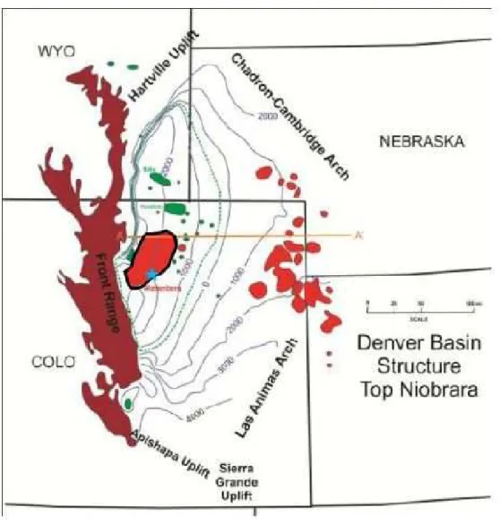
Wattenberg Field is located in northeast Colorado in the Denver Basin (Figure 1.1). It covers more than 2,000 square miles between Denver and the town of Greeley. Over 20,000 wells have produced from Cretaceous formations in this field. The majority of drilling occurs in Weld County, but development also stretches into Adams, Boulder, Broomfield, Denver, and Larimer Counties.
The Niobrara Formation is one of many formations that are productive in this field, and is a major tight, petroleum resource play. The Niobrara, along with the underlying Codell Sandstone, is the reservoir of interest in this study. The Niobrara consists of interbedded
Figure 1.1: Map of Wattenberg Field outlined in black (Sonnenberg, 2013). Blue star indi-cates study area.
ologic heterogeneity is the main reason for the production variance within the Niobrara. Not only are there multiple chalk and marl benches, but within each bench there are very thin chalk and marl layers. The Niobrara has very low porosity (8-10%) and permeability (0.1md), which makes it an unconventional play (Sonnenberg, 2013). The overlying Lower Pierre Shale is also an important formation in this study due to the overpressure observed. The area of interest for this research is focused over four square miles in the southeast cor-ner of Wattenberg Field. The project sponsor, Anadarko Petroleum Corporation (APC),
has provided multiple datasets to RCP to aid in interpretation that will ultimately lead to understanding the stimulated areas of the reservoir. Integration of geology, geophysics, and petroleum engineering is a critical component for understanding unconventional fields like Wattenberg. The key objective of the Wattenberg project is to determine how faults and natural fractures affect the reservoir. In addition, there is a need in understanding how stress state changes over time and identify how the formation heterogeneity influences completions and production. APC has drilled 11 horizontal wells in section 24 of T2N66W, called the Wishbone section (Figure 1.2). The project focuses around the data from these wells to understand their completion performance. They were completed from east to west in fall of 2013. A timeline of when these wells were drilled and seismic data was acquired is shown in Figure 1.3. Preliminary results show that there is a high degree of complexity within the reservoir, due to multiple fracture networks and heterogeneity of the chalk and marl layers. There is also potential hydraulic connectivity between the Niobrara and Codell formations. To capture a full understanding of the reservoir heterogeneity of the field, the variations in geomechanical and petrophyscial properties need to be analyzed. Data include seismic, microseismic, well logs, image logs, tracer data and production data. Several seismic surveys were acquired (Figure 1.4) and are listed in Table 1.1. The area of interest for this research is within the time-lapse, multicomponent survey over the Turkey Shoot region. Time-lapse data are vital for this research to help determine changes in the reservoir with respect to time. The stimulated and produced areas of the reservoir can be determined with proper analysis of time-lapse data. These 3D seismic surveys include PP, PS and SS wave datasets. Shear data are useful for determining fracture orientation and density. Compressional data can be used, in a time-lapse sense, to locate what portions of the reservoir have been affected by production. The engineering data for the wells includes completions reports, tracer and production data. Well logs for the horizontal wells and vertical wells in the area were pro-vided. Using well data and seismic data are important in interpretation, because it allows for an understanding of the reservoir at both a large and small scale. The relationship between
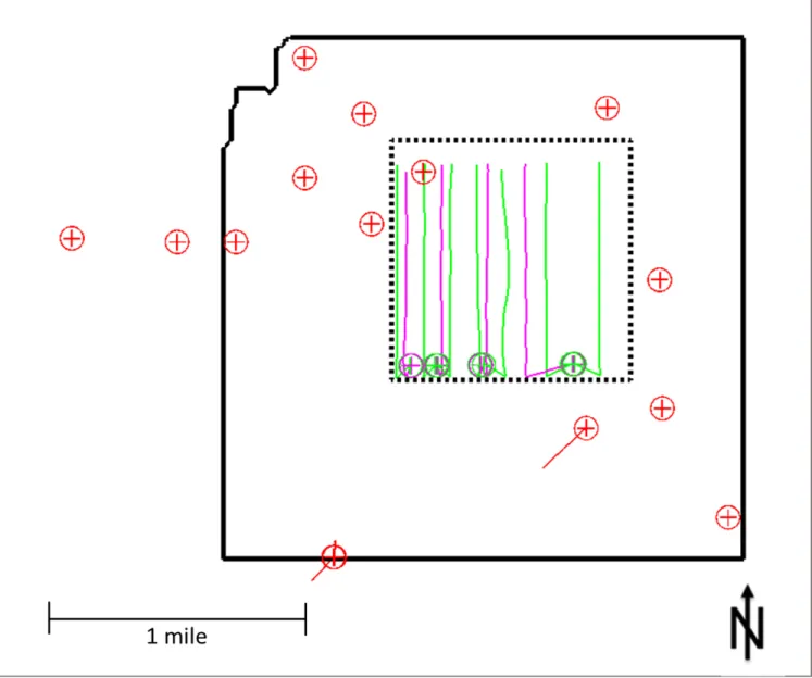
Figure 1.2: Wells of interest in Turkey Shoot (solid line), Wishbone (dashed line). Vertical wells in red, Niobrara horizontal wells in green, and Codell horizontal wells in pink.
the stress field and geomechanical properties with production and hydraulic fracturing has been investigated in this research study.
1.3 Geologic History
The Denver Basin is a 70,000 square mile, asymmetrical basin of Laramide age. It is an elongated shape stretching north to south, which has a steeply dipping western flank and gently dipping eastern flank; spanning throughout portions of Colorado, Wyoming and
Figure 1.3: Timeline of seismic acquisition and well development.
Table 1.1: Geophysical surveys
Survey Name Areal Coverage (sq. mi.) Type of Survey
Regional (Merge) 50 WAZ 3D/1C
Anatoli 10 3D/3C
Turkey Shoot 4 4D/9C
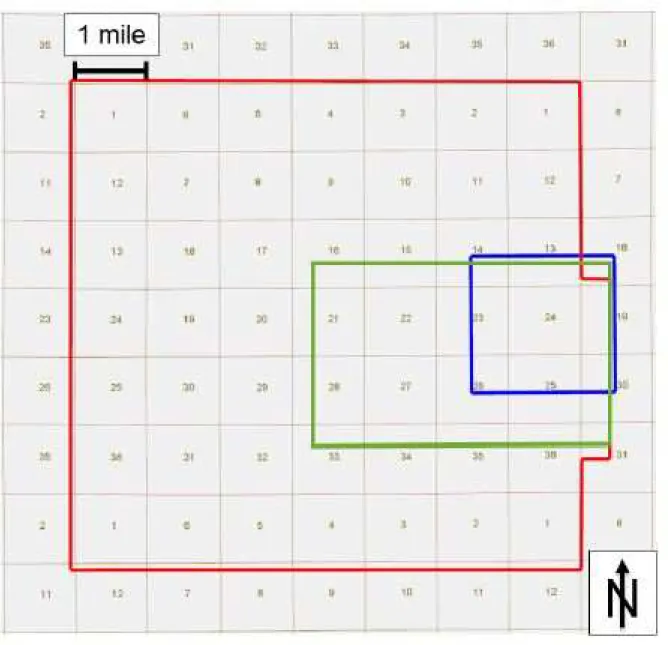
Figure 1.4: Map of seismic surveys. Red = Merge. Green = Anatoli. Blue = Turkey Shoot.
Nebraska. The basin is bounded to the west by the Rockies front range, Apishapa uplift and Hartville uplift, and to the east by the Chadron arch and Las Animas arch. The formation of the Denver Basin was part of the Ancestral Rockies, and was later deepened during the Laramide Orogeny; the creation of the modern Colorado Rockies. The basin was later filled with sediment that eroded from the Rockies. Sediment packages are thickest along the basin axis, a line between Denver and Cheyenne, due to this alluvial fan type deposition. These
sediments consist mainly of sandstone, shales and limestone, overlying Precambrian rocks that form the basement as deep as 13,000 feet beneath the surface.
The Denver Basin contains about 1,500 oil and gas fields, where the majority of hy-drocarbons are produced from reservoirs ranging in age between Paleozoic and Cretaceous. Conventional exploration has historically been focused in the Lower Cretaceous Muddy J and D sandstones (Weimer et al., 1986). Intense exploration and drilling began in these reservoirs in the early 1950s. The Wattenberg Field is considered an unconventional field due to the tight nature of the Niobrara, Codell and J formations. The field is considered a low permeability basin center gas field, where these basin centered accumulations in the Niobrara and Codell reservoirs have been the main target in Wattenberg. The first well was drilled in 1970 (Weimer et al., 1986), but exploration was slow for the Niobrara and Codell Formations until the early 1980s. At this time drilling rates began to increase due to an increase in oil price and Federal pricing incentives for tight reservoirs. With the discovery of sweet spots and combined production from Niobrara, Codell and underlying Muddy J, the amount of drilling in the field exponentially increased.
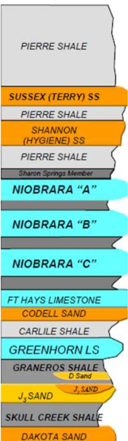
The thickness of the Niobrara in Wattenberg Field ranges from 240-330 feet. Production is predominantly from four chalk layers within the Niobrara that are typically each 20-30 feet thick. These four chalk layers, or benches, are labeled as A, B, C and D chalk (Figure 1.5). It should be noted that the area of Wattenberg Field in which this study was conducted the A chalk layer does not exist. The Codell is considered a siltstone and ranges from 15-25 feet in thickness. As mentioned before, these reservoirs have very low porosity and permeability (Sonnenberg, 2013), where the Niobrara is 10% and less than 0.1mD respectively, as well as the Codell at 14% and 0.1mD respectively. The unconventional nature of the Niobrara and Codell reservoirs makes it extremely difficult to produce hydrocarbons without hydraulic fracturing.
Several reasons for higher production in an unconventional formation include, large frac-ture density and a more open network fracfrac-ture system, better grain sorting with lower
amounts of matrix clays and muds, and an overall thicker reservoir section. Within the Wattenberg Field, oil and gas are stratigraphically trapped in nearshore, marine sandstone intervals of the Codell. The hydrocarbons are surrounded by impermeable rock, making them virtually immobile. Fractured sands, limestones and shales make up the reservoir in-tervals of the Niobrara. The Mowry and Graneros shales are the main source rocks for all Lower Cretaceous formations. The Upper Cretaceous formations are sourced by some of the Lower Cretaceous reservoirs, including the Niobrara, Carlile shale and Greenhorn limestone. Any Paleozoic reservoirs are most likely sourced from Paleozoic black shales.
1.4 Stress History
Studies have shown that understanding the stress state and tectonic history of a reservoir is important for optimizing development. Knowing the timing of faults and other structures can lead to conclusions about stress changes, deformation and geomechanical changes. The depositional, burial, and stress history are all interrelated and can show how a formation has been altered, mechanically and chemically, over millions of years. This will ultimately lead to the understanding of the present day stress state of the field, and the areas for optimal production and hydraulic fracturing. The Niobrara is a Cretaceous age formation and was deposited in a foreland basin in the Western Interior Seaway. This was a time of a marine transgression and represents a maximum sea-level highstand.
The basins currently present, throughout the Rocky Mountain region, were formed dur-ing the Laramide orogeny. The Western Interior Cretaceous basin was bordered to the west by plutonism, volcanism, and thrusting, and to the east by a broad cratonic zone. This basin had experienced the effects of sediment loading and rapid subduction with drastic subsidence (Sonnenberg, 2013). Niobrara lithology consists of limestone, with interbedded marl layers. These rocks naturally have low porosity, but with diagenesis, pore throat sizes were reduced even further. This is one of the main reasons fracturing is needed to create a productive reservoir. Fault systems, determined by seismic data, are present in the Nio-brara interval. The majority of faults seen are normal and slightly listric. Shear or wrench
Figure 1.5: Stratigraphic column of Wattenberg Field (Sonnenberg, 2013). The Niobrara A Chalk is not present in this study area.
faults were also observed within the Wattenberg area. Many faults dip at approximately 45 degrees, are slightly listric, and influence fractures within the Niobrara formation (Davis, 1985). Polygonal fault systems are also present in Wattenberg Field. These are mainly
interpreted from 3D seismic data. Two polygonal faults, creating a large graben, are located in the Wishbone section and penetrate the Niobrara interval. In general, formations above and below the Niobrara interval were not affected by polygonal faulting. Students in RCP have been actively studying the fault framework and stress state of the Niobrara. The key objective for the Wattenberg project are determining how faults and natural fractures affect the reservoir and how the stress state changes through time. Initial conclusions, thus far, include: complex natural and induced fractures are present, shear seismic data can define fractures more clearly than compressional seismic, there is a connection between short-term initial production and 4D effects, and the general azimuth of maximum horizontal stress is approximately N65◦W, which was determined using image logs and microseismic. The initial stress state determined from seismic data corresponded well with data from the easternmost wells within Turkey Shoot, but not with the western wells. This is due to maximum and minimum horizontal stress direction alterations from the hydraulic fracturing operations. The easternmost wells were completed first, therefore changing the initial stress state for the western wells. This is an area of study that needs to be better understood. Every time hydraulic fracturing takes place, there is a change to the stress state in the formation. If the nature of this change could be mapped and quantified, the stimulated reservoir volume could be better estimated.
1.5 Methodology
The main objectives of this thesis study are to identify geomechanical and stress dis-tributions throughout the reservoir, how stress alterations are related to the geomechanical properties and how this relationship can help to determine optimum well locations and their spacing. The methodology used for this study was divided into five main areas of research: data inventory, stress analysis, structural modeling, stress simulations, and finally analysis and recommendations.
1.5.1 Data Inventory
At the initial stage of any project it is important to determine the data available, what conditioning must be applied to the data, and the previous work conducted in the same area. There are many different types of datasets that have been made available to RCP by the project sponsor, APC. The data crucial to this thesis study are seismic volumes, well logs, and well completions and production data. Prior work important to this thesis includes initial structural models, petrophysical analysis of the Wattenberg project, and theses studies completed in the past on related topics. A model framework, created by Pitcher (2015) is used as the preliminary steps for the models created in this study. Understanding the well data in the area is also important before making any interpretations. Five wells were used in the creation of the initial model, but more well data was desired. There were ten additional wells in the Turkey Shoot area. In order to use these wells for interpretation, well normalization needed to occur. The vertical wells in this area have been logged by various companies and it is important to calibrate well data for the interpretations between the wells to be reliable. Other data available in the Wattenberg project include microseismic, image logs, core, and tracer data. These additional data will be important to use as validation data for the conclusions reached in this study.
1.5.2 Stress Analysis
Determining the stress regime and stress anisotropy of a reservoir is crucial to understand the formation geomechanics and associated design and execution for the operations. Quan-titative stress magnitudes are quite difficult to obtain. In this thesis study, linear elastic assumptions for the reservoir formation were used to estimate stress magnitudes and overall stress anisotropy throughout the reservoir. Completion data has also been taken into ac-count to understand what reservoir parameters have the greatest impact on the stress and pressure trends. Net pressure trends, from these completions reports, have been analyzed to understand fracture propagation throughout the reservoir.
1.5.3 Structural Modeling
The creation of a geological model is the next step. A model helps to look at the reservoir interval and other formations of interest in a 3D view. It can incorporate horizons, faults, and well data and can be as simple or complex as the user desires. This structural model will allow the interpreter to visualize the area of interest spatially or in a cross section view. Future use for a structural model in this study is to incorporate it into reservoir geomechanics and production simulations. A model that can accurately represent the Turkey Shoot study area can be tested in simulations that will show stress magnitude changes, and potentially Stimulated Reservoir Volume (SRV).
1.5.4 Simulations
There are different types of simulations that can be performed depending on the de-sired outputs. Depending on the simulation used it can account for many factors such as, oil production, fluid injection, drainage area, etc. For this project the goal has been to perform simulations that will detect changes to the stress field within the study area. Pre-liminary stress simulations will be analyzed mainly with the reservoir geomechanics module in PetrelTM
. This module has the capability of modeling formations around the reservoir to better describe far field stresses. As a reservoir depletes, effective stress changes, and sometimes even causes stress reversal. The goal of running simulations is to better predict where rocks will fail, where to target hydraulic fracturing efforts, and how the geomechanical properties are changing through time in the reservoir. This research provides insight on the simulation process and what information could be provided from full simulation runs by future RCP students.
1.5.5 Analysis and Recommendations
The final portion of this report will be the examination of results. Analysis will be based upon the findings from field background research, previous work, the stress analysis and the modeling results. Relationships between the stress anisotropy, acoustic properties
and petrophysical properties will be discussed in an attempt to aid in optimization of the future drilling and completion designs. The analysis portion of the report will also provide recommendations for future work.
CHAPTER 2 LITERATURE REVIEW
Geomechanics plays an important role in the production of hydrocarbons. It is the bridge between geophysical observations and reservoir engineering applications. Reservoir geomechanics is a study of how stresses, temperatures and pressures change and affect the mechanical and petrophysical properties of rocks. It is important to assess the initial con-ditions of the reservoir and use known geomechanical properties to try and predict how the formation will change due to drilling, stimulation and production. In this thesis study, geomechanical properties and stress changes of the Niobrara Formation within the Turkey Shoot region have been investigated.
2.1 Geomechanics in Unconventional Reservoirs
Unconventional reservoirs have become a crucial part of the portfolio of many oil and gas companies. Producing from a shale formation requires more complicated completion techniques than conventional production. Hydraulic fracturing is a necessity when it comes to producing from these tight, non-permeable, reservoirs. The Niobrara in Wattenberg Field, falls into this category, as mentioned in the previous chapter. Understanding the geomechanics of the producing interval, as well as the overburden and underburden, are vital when planning completion methods. Geomechanical properties not only help predict how the rock will react under a given stress state, but also in predicting wellbore stability, high or low pressure zones and reducing other drilling risks.
Unconventional formations span far and wide in composition, depositional history, min-eralogy, and their rock properties. All of these can have an effect on the geomechanical properties. Shales are not stratigraphically or spatially homogenous, nor were they deposited solely by hemipelagic sediment in a quiet, deep marine environment, as has been tradition-ally thought (Slatt and Abousleiman, 2011). It is important to gather as much information
as possible that can help in the prediction of how the reservoir will behave due to stimulation and production. Geomechanics plays a significant role in unconventional production, partic-ularly because of the need for hydraulic fracturing and the associated alterations that take place even before production starts from the reservoir. With even a basic understanding of the geomechanical properties of the reservoir, an optimal and more efficient well plan and design can be implemented.
2.2 Geomechanical Properties and Stress Equations
There are several geomechanical properties used to describe the behavior of a formation. The two most common geomechanical properties include Young’s Modulus and Poisson’s Ratio. These properties are calculated using seismic velocities and formation density to characterize the compressibility and brittleness of the reservoir. Young’s Modulus (E) is a measure of stiffness and Poisson’s Ratio (ν) is the ratio of expansion over compression (Ramsey, 2016). E = ρV 2 s(3V 2 p − 4V 2 s) V2 p − V 2 s (2.1) ν = V 2 p − 2V 2 s 2(V2 p − V 2 s) (2.2)
The variables ρ, Vp and Vs represent bulk density, compressional velocity and shear velocity respectively.
Ideal values for these properties are a low Poisson’s Ratio and high Young’s Modulus (Figure 2.1). At a fixed stress state this would indicate a brittle formation that would more easily fracture. It is important to note though, that a material can be made brittle by varying stress state, temperature, fluid type and mineralogy. Also, if a formation is already fractured then understanding these fractured sweet spots may carry vast importance. Young’s Modulus
and Poisson’s Ratio can be useful guides when analyzing areas that may fracture easier, but other rock properties must also be taken into account.
Figure 2.1: Young’s Modulus vs. Poisson’s Ratio. Arrow pointing in the direction of in-creasing brittleness for a fixed stress state.
The next important set of equations to understand are earth stresses. Depending on geomechanical properties, a rock will fail when it has undergone certain stress and pressure. Knowing rock failure parameters is extremely important when drilling a well, to avoid well-bore damage, and also for hydraulic fracturing, to predict when the formation will fracture. The first step in predicting stress is through linear elastic theory. An elastic object is one that will eventually return to its original shape, after undergoing slight deformation by an outside stress. Hooke’s Law uses this theory to describe a stress-strain relationship of which the deformation of an elastic object is proportional to the stress applied to it (Higgins et al., 2008).
σij = Cijklǫkl (2.3)
The variables σ and ǫ denote the second rank stress and strain tensor. The stiffness tensor, C, can be defined for an arbitrary material using the following matrix.
C11 C12 C13 0 0 0 C21 C22 C23 0 0 0 C31 C32 C33 0 0 0 0 0 0 C44 0 0 0 0 0 0 C55 0 0 0 0 0 0 C66
According to Bratton (2016), linear elastic theory is used to analyze the stress state that causes drilling induced damage. Positive numbers should be used for compressive stresses and negative numbers for tensile stresses. There are many types of shear and tensile failure modes, and the more information the driller has about these failures, the safer and more effective the drilling and completion process can be. Pore pressure, the pressure of fluids within the pores of a reservoir (Ramsey, 2016), is also critical to know before drilling a well. Radial wellbore stress is described by the following equation.
σ′
r = Pw− Pp (2.4)
Pw and Pp denote wellbore stress and pore pressure.
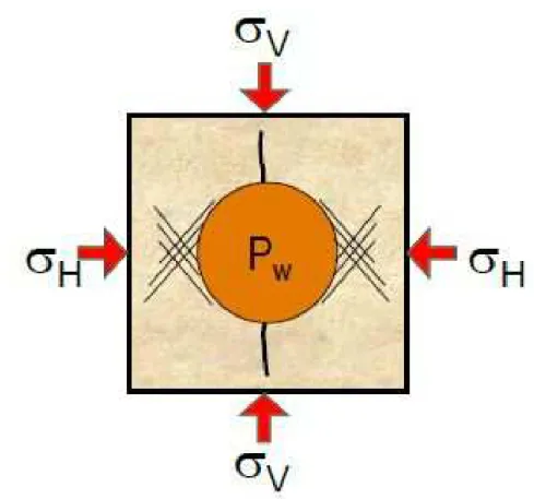
There are two sets of stresses used in the analysis of wellbore stability, far-field stresses and wellbore stresses. Far-field stresses occur naturally in the earth, but can be altered around the wellbore due to drilling through the rock and the injection of drilling fluid into the reservoir. There are three far-field stresses, vertical (σv), maximum horizontal (σH), and minimum horizontal (σh).
Figure 2.2 demonstrates the principal stresses in a normal fault regime, which is the stress state of the Wattenberg study area, and overall Denver Basin.
Figure 2.2: Principal stresses acting on a normal fault, as described by the Anderson fault classification system.
There are several assumptions required for hydraulic fracturing (Harrison and Hudson, 2000). The first is that one principal stress is vertical and is due to the weight of the overburden. Another assumption is that the rock is impermeable and fractures will be formed in a vertical plane. Lastly, Kirsch equations (described below), can be used to estimate the stress concentration around the borehole. This will be with the assumption that the formation is linearly elastic.
For an estimation of overburden stress, σv can be calculated with bulk density, ρ, the gravitational constant, g, and true vertical depth, h.
From the Kirsch equations (Harrison and Hudson, 2000), minimum and maximum hori-zontal stresses can be used to predict when a rock will fail. Tangential wellbore stress (σ′
θH), or ”hoop” stress must be overcome for breakdown to take place. Hoop stress can be described from the following equation for a vertical well:
σ′
θH = 3σh− σH − Pw− Pp (2.6)
Figure 2.3 demonstrates the principal stresses acting on a vertical well.
Figure 2.3: Diagram of principal stresses for a vertical well.
In this study, the wells are horizontal and therefore a slight variation of this equation is used. The maximum principal stress in this field is σv, and the horizontal wells are drilled in a direction closely aligned with σh. This means that σh will not have as great of an effect
σ′
θH = 3σH − σv− Pw − Pp (2.7)
Figure 2.4 demonstrates the principal stresses acting on a horizontal well aligned with minimum horizontal stress.
Figure 2.4: Diagram of principal stresses for a horizontal well aligned with minimum hori-zontal stress.
Linear elastic equations are useful when trying to form a general understanding of the far-field stresses in a field of interest, but it is understood that shales exhibit anisotropic behavior. Shales are often described by transverse isotropy, which characterizes a rock that has an axis of symmetry where the rock property is the same in two directions but not the third (Higgins et al., 2008). It also indicates that when the rock is fractured, it does not completely return back to its original shape. As the shear stress increases and the yield
strength of the formation is exceeded, the grains begin to re-orient, and will not return back to their original state.
2.3 Role of Geomechanics in Hydraulic Fracturing
Due to the tight, impermeable nature of these reservoirs, like the Niobrara, hydraulic fracturing is used during the completion process. Hydraulic fracturing has become the key to unlocking unconventional resources, however the fracturing process is the most poorly understand feature of the drilling and completion process (Curnow and Tutuncu, 2016). In an attempt to predict how a formation will break under stress, the geomechanical properties must be understood. Predictions become even more complex when dealing with a naturally fractured reservoir. One of the goals of this project is to better predict the interactions between the hydraulic and natural fractures. Based on shear data analysis from Motamedi (2015), it is known that the Niobrara is a naturally fractured reservoir. Where exactly the most natural fractures occur is still uncertain, therefore, an analysis has been conducted in this project. Different formations will have different natural fracture systems, with varying aperture and connectivity, which will depend on the geomechanical properties of the forma-tion, along with the maximum and minimum horizontal stress magnitudes and orientations. Extensional fractures will propagate in the direction of maximum horizontal stress and open in the direction of minimum horizontal stress. Shear fractures, on the other hand, will occur obliquely to the maximum horizontal stress direction. Properties such as Young’s Modu-lus and Poisson’s Ratio have a large impact on the in-situ stress state (Gray et al., 2012). For example, a larger Poisson’s Ratio usually indicates a more ductile rock, and therefore a larger stress is required to fracture the rock. Microseismic is another tool used to analyze fracture systems and should follow the maximum horizontal stress direction. According to Lorenz (2016), the stronger the stress anisotropy, the more linear the microseismic response is. Hydraulic fractures are expected to follow the direction of natural fractures, but this is not always the case. If stress anisotropy is low and the fracture fabric is strong, the
forma-maximum horizontal stress. Before moving forward with the hydraulic fracturing process it is important to create a drilling and completion design that will honor the in-situ forma-tion properties and have the most fracturing potential. Factors that need to be considered include well direction and spacing, hydraulic fracturing stage length, injection rate, fluid volume, among others.
2.4 Stress Shadow Effect
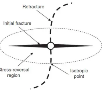
Stress reorientation is a topic that has become popular in the past few years. It is known as stress shadow effect and is defined as a redistribution of stresses around a fractured well due to nonuniform depletion of a reservoir (Roussel and Sharma, 2012). Initially, fractures are created in the direction of maximum horizontal stress and open in the direction of minimum horizontal stress. During production operations the maximum horizontal stress decreases faster than the minimum horizontal stress, because the fluid will be able to travel faster in the fracture direction. This may cause stress reversal in the vicinity of the fracture. When a fracturing job is completed, fluid pressure in the reservoir drops and the fractures created will close down on the injected proppant. The new stresses will now be higher in the direction of in-situ minimum horizontal stress. When this occurs, stress reversal will take place. The distance away from the wellbore that this stress reversal will reach is greatly dependent on the geomechanical properties and stress anisotropy of the reservoir. Initially, brittle rock will be easier to fracture, and then the magnitudes of the principal stresses will determine the stress reversal region. It may be possible for the stress reversal region to even be larger than the fracture half-length, but this will depend on fracture height and width, and Young’s modulus in the pay zone (Roussel and Sharma, 2012). At some point, the stress reversal will end and there will be virgin rock that has the intact in-situ stress values. With a re-fracturing effort, this virgin rock may be reached, and a new set of fractures can be exploited. The timing for re-fracturing is another highly debated concept, but is beyond the scope of this research. Figure 2.5 is a schematic of a second fracture propagating orthogonally to the initial fracture in a re-fracturing effort.
Figure 2.5: Schematic of an initial and secondary fracture from a re-fracturing effort (Roussel and Sharma, 2012).
Within the study area of Wattenberg Field, it is believed that stress anisotropy is fairly low, based on the pressure data, like the instantaneous shut in pressure values (ISIP) when implemented in the Kirsch equations. Part of this study is to determine if stress reversal is possible in this region and how geology plays a part in the stress regime change. If in-situ stress and stress reversal can be understood in the Niobrara, more efficient well drilling and completion designs may be implemented.
CHAPTER 3 STRESS ANALYSIS
Stress is a complicated topic because it can be affected by so many variables. Even when dealing with an isotropic, homogeneous formation, stress is influenced by reservoir depth, rock strength, age, tectonic history and many other factors. The Niobrara is a heterogeneous reservoir, and is influenced by fault compartmentalization. Calculating the stress accurately in this environment is quite difficult. As mentioned in the previous chapter, using linearly elastic assumptions to obtain an answer is still a good starting point. Also, completion data can be used to analyze breakdown pressure and ISIP data that can lead to a prediction of maximum and minimum horizontal stress. This chapter looks into using field reports to link pressure data to stress and fracture behavior in the Wishbone section of Wattenberg Field. 3.1 Completion Reports
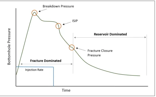
Completion reports have been provided to aid in reservoir characterization of the Wish-bone section. The 11 APC wells were completed with hydraulic fracturing techniques by Halliburton. These reports provide treatment and pressure plots at every stage for all 11 wells and notes about the individual fracture jobs. A map view of the wells is shown in Figure 3.1. Ten of the wells were fractured using one completion technique, and one well (9N) was completed with a different method. A typical treatment plot will show bottom hole pressure throughout the time it takes to complete the stage. Several types of pressure points can be interpreted from this timeline. An example treatment plot is shown in Figure 3.2. The most important information obtained by the treatment plots is the breakdown pressure, ISIP, and the closure pressure. Breakdown pressure is the pressure needed to initially break the rock; ISIP is the final injection pressure minus pressure drop due to friction and per-forations in the wellbore; and closure pressure is the pressure needed to keep the fracture open.
Figure 3.1: 11 wells within the Wishbone section.
Figure 3.2: Example treatment plot. From this pressure curve values such as breakdown pressure, ISIP and closure pressure can be determined.
3.2 Net Pressure Trends
Net pressure plots were provided with the completion reports and show the overall pres-sure trend throughout the entire stage. If the prespres-sure trend is increasing this means the fracture most likely stayed in the anticipated zone and fluid pressure had built up. If the pressure trend is decreasing, the fracture may have broken out of the zone and might have grown into a different lithology, or could be opening pre-existing fractures. In some uncon-ventional fields, if the producing interval is a thin layer surrounded by poor quality rock, that may be a negative result. In the case of Wattenberg Field, the Niobrara is comprised of alternating layers of chalks and marls, all of which are considered productive, and also overlays the Codell sandstone. A decreasing trend in net pressure could be a positive effect in this situation, because it probably means the fracture is propagating through multiple layers. Nolte and Smith (1981) published a paper which analyzed these net pressure trends. Net pressure is defined as the pressure in the fracture minus the in-situ stress. In their paper, interpreting net pressure behavior in the field is presented to determine estimates of frac-ture growth patterns. They assume that as long as the fracfrac-ture height is contained, the net pressure will increase with time. This study was conducted for a homogeneous reservoir, but general pressure trends can help to understand fracture behavior in heterogeneous reservoirs as well, such as the Niobrara Formation. Figure 3.3 is a graph describing the four trends observed in net pressure plots and how they pertain to fracture growth. Mode I represents normal lateral fracture growth. Mode II can be stable height growth or increased fluid loss, but has less lateral growth than Mode I. In Mode II the fracture can still propagate and be filled with proppant. Mode III represents a fracture that has stopped propagating and is being inflated as the net pressure increases. With this mode, proppant can still be injected, but the pressure must be monitored closely to ensure maximum injection pressure is not reached. With Mode III, if the net pressure slope is greater than one, a screen out may occur. This is a condition where the solids carried in a treatment fluid, such as proppant, create a bridge across the perforations. This creates a sudden and significant restriction to
fluid flow that causes a rapid rise in pump pressure (Ramsey, 2016). If a net pressure plot replicates the trend of Mode IV, the fracture height is increasing rapidly (Nolte and Smith, 1981).
Figure 3.3: Net pressure trends (Williams et al., 1979). Mode I - Normal lateral fracture growth. Mode II - Less lateral fracture growth. Mode III - Lateral fracture growth has stopped and pressure is increasing rapidly. Mode IV - Rapid fracture height growth.
In this study, completion reports were analyzed for wells 1N, 2N, 6N, 7N and 9N. These five wells were chosen because they were the wells drilled most consistently through the Niobrara target interval, the C Chalk. Figure 3.4 shows the 11 Wishbone wells color coded by the lithology at each stage. White (2016) developed this figure after analysis of the geosteering reports.
The net pressure plot for each stage was associated with one of the four different Nolte and Smith (1981) modes for fracture characterization. Figure 3.5 shows an example net pressure plot for each mode from well 1N.
Figure 3.4: 11 Wishbone wells with stages color coded by lithology (White, 2016). Map is a time slice through an incoherence volume for the top Niobrara (Pitcher, 2015).
There was no net pressure trend that was consistent for each lithology, but there was a slight trend when near or inside the major Wishbone graben. Figure 3.6 displays the stages for wells 1N, 2N, 6N, 7N and 9N color coded by net pressure mode. When looking closely at the central graben, it seems that most stages represent Mode I, or at least Modes I-III (Figure 3.7). Modes I and II show normal lateral fracture growth, and Mode III means the fracture has stopped propagating and there is a net pressure build up. Many of the stages outside the graben are Mode IV, which means fracture height is increasing rapidly. This difference in net pressure trends helps validate the idea that fault compartmentalization is present in the Wishbone. There is a larger net pressure trend within the graben, which means those faults could be barriers to flow. There may be pressure build up inside the fault due to the fracturing of multiple wells inside the graben. Net pressure is associated with fracture characterization, which is ultimately related to geomechanical properties. There is most likely a change in rock mechanics inside and outside of the graben. Another interesting
Figure 3.5: Net pressure plots from different stages for well 1N, each representing a different Nolte and Smith (1981) fracture characterization mode.
observation is that the wells on the western side of Wishbone, 7N and 9N, have mostly decreasing net pressure trends. This could mean one of two things. First, it could mean the standard Mode IV definition; fracture height is rapidly increasing. Second, it could mean these fractures are penetrating depleted zones. There are several horizontal wells that exist in the section to the west of Wishbone. Depending on the stimulated reservoir volume (SRV) of those wells, they may have depleted areas of western Wishbone. If wells 7N or 9N where fractured into these zones, a decreasing net pressure trend would be seen. This is quite unlikely though, because the wells were completed around the same time.
Net pressure plots were analyzed for increasing or decreasing trends throughout the time it took to complete each stage. The main observation was found near the central graben
and western side of Wishbone. There was a consistent increasing pressure trend inside the graben, for the five wells analyzed, and mainly decreasing trend just outside the graben (Figure 3.7). Also, overall decreasing net pressure trends were observed throughout the 7N and 9N wells. This is associated with height growth; possibly leading to connectivity between the Niobrara and Codell reservoirs in this region.
One of the main goals of the Wattenberg project is to understand how the geology affects production. The idea that this central graben has a large influence in the Wishbone section is supported in many analyses. The difference in net pressure, described in this chapter, caters to the idea that fault compartmentalization is present in the Wishbone section. These conclusions are compared to other RCP studies later in this thesis.
Figure 3.7: Stages for wells 1N, 2N, 6N, 7N and 9N color coded by net pressure trend mode. Modes I-III in graben highlighted in red.
CHAPTER 4 MODELING PROCESS
The main focus of this research is to create a structural model, representing the Turkey Shoot region, which could later be used in various engineering and geomechanical simulations. A major goal of the entire Wattenberg project has been to model the subsurface as closely as possible, and try to predict the rock behavior under stress. There are many steps that go into creating a model, and several students have contributed to portions of this process. This structural model is dynamic, and can constantly be updated with new information, modified inputs, and more properties over time. The hope is that this model will stay within the RCP Wattenberg project, and each year there will be new additions or results that are obtained from it.
4.1 Data Collection and Well Normalization
The first step in any modeling process is to understand what data are available, if any corrections must be applied and what previous work has been done. The data used in this model consists of well data, seismic interpretations, such as horizons and faults, and seismic inversion properties. An initial model was created by a former RCP student (Pitcher, 2015), and that model development strategy was used in this project. Work by other students, including horizons, faults, velocity models and inversions are mentioned later in this chapter. Properties from five wells were used to populate the initial model, but more well data was desired. There were ten additional wells in the Turkey Shoot area, but before incorporating them into the model they needed to be normalized. Many of the vertical wells in this field have been logged by different companies and it is important to calibrate their data before loading them into the model. Figure 4.1 is a map of the vertical wells used in the normalization process for the Turkey Shoot area. Well normalization is a key process that needs to be completed before data analysis. It optimizes well log data to accentuate geologic
responses while minimizing error effects. Incorrect interpretations may be made if data are not calibrated properly and if wells were poorly and inconsistently normalized. Normalization is adjusting for error, which could have occurred for a variety of reasons: borehole conditions, well log vintage, well logging company, etc. Environmental corrections must be made along with any shifting of data due to which rock matrix a certain tool was calibrated to.
Within Wattenberg Field, specifically Turkey Shoot, there are several different service companies that have logged the vertical wells in the survey area. Phoenix wells, for example, tend to be logged using tools much older than Schlumberger. The difference in tools used has a great effect on the data recorded. An important aspect of the normalization process is knowing what zones to normalize. Zones should be based on the consistency of rock properties throughout the field. In the Turkey Shoot, wells were normalized using the Lower Pierre and Ft. Hayes zones. These zones have little variability across the study area. The well log signatures were relatively the same across the vertical wells.
The Niobrara was not chosen as a zone to normalize, because it is expected that there will be variability in reservoir intervals. Wells were normalized using a quantile two-point shift in TechlogTM
. A minimum and maximum point could be set on the calibration well where the other wells would be normalized to. This caused a slight shift in values in the Phoenix wells. These shifts were monitored using histograms of the well log data of interest: gamma ray, density, neutron porosity and resistivity. Figure 4.2 is an example of well normalization histograms. The wells shown in Figure 4.1 were normalized in this project and then incorporated into the model. The calibration of well data was the main task in the data inventory process. Once this was completed, the structural modeling process could begin.
4.2 Structural Model
The structural modeling process was completed in the Schlumberger software PetrelTM . PetrelTM
Figure 4.2: Example histograms of well normalization for Gamma Ray log. Zone of normal-ization is Lower Pierre. Phoenix wells in pink, Schlumberger calibration well in blue.
contracts with CSM, PetrelTM
was the software of choice. There are many inputs for a geocelluar, structural model, but the process is fairly straightforward. Figure 4.3 displays the workflow for creating a model in PetrelTM
. 4.2.1 Wells
The first step is to import well data. Once wells were normalized in TechlogTM
, they were exported in proper ASCII file format in preparation to be imported to PetrelTM
. Deviation logs provide the X, Y and Z coordinates for the entire well, to ensure the well is imported to the proper location. Another important parameter is the kelly bushing height. This is the distance off the ground that the kelly bushing sits, and technically where measured depth for the well begins. This value must be taken into account when importing wells so that the surface location is correct.
Once the wells are in their proper location, the logs associated with them can be imported. Logs such as gamma ray, deep resistivity, bulk density, neutron porosity and many others were incorporated into the project.
4.2.2 Core
The research presented here incorporates geomechanical properties calculated using dy-namic data; sonic logs and seismic. In modeling it is important to understand the static data as well. Dynamic data changes through time, whereas static data does not. Unfortunately, there are no cored wells in the Turkey Shoot. The closest cored well is the Core Well #3 (Fig-ure 4.4), approximately four miles north of Turkey Shoot. Another RCP student conducted research that incorporated core measurements from Core Well #3. These measurements consisted of using a Proceq Bambino, hand-held rebound hammer, which can measure brit-tleness through non-destructive testing. Hardness values can be read from the hammer and converted to confined compressive strength (CCS). The hardness values represent the ratio of rebound velocity to impact velocity (Murray, 2015). Bambino testing and triaxial stress tests on Niobrara cores in other fields have yielded a relationship that converts hardness to CCS. Once CCS values have been determined they can be compared with geomechanical properties calculated from well logs. Figure 4.5 displays well information from Core Well #3 (Mabrey, 2016). CCS values, determined from core data, are overlain onto geomechanical property logs calculated from sonic.
Figure 4.5: Core Well #3 logs. Black data points represent CCS values determined from core testing (Mabrey, 2016).
The three tracks on the right show CCS and several types of bulk moduli. The curves will not be the same values but their general trends should align fairly well. As seen in Figure 4.5, the CCS curve follows the trends of the Young’s Modulus, Bulk Modulus and Poisson’s Ratio curves quite consistently, especially within the chalk layers. It was determined that the dynamic logs of Core Well #3 represent the static data from core. The dynamic data were incorporated into the structural model.
4.2.3 Seismic
The next step is to collect the proper seismic information. Several students have created interpretations using the seismic surveys provided by APC. Faults interpreted by Yanrui Ning and horizons interpreted by Payson Todd, on the Turkey Shoot PP baseline survey, were used in this model. There were 18 major faults in the Turkey Shoot region. The faults and horizons were interpreted in time, and so depth conversion was needed in order to proceed with the modeling process. Payson Todd developed a velocity model from 13 well ties in the Turkey Shoot area. This velocity model was used to depth convert the faults and horizons used in the structural model. Figure 4.6 displays the wells used in the velocity model.
4.2.4 Model
In order to construct a grid of the Turkey Shoot, a zone model was created based upon horizons and faults. Horizons used include: Mid-Lower Pierre, Sharon Springs, Niobrara Top, B chalk, B marl, C chalk, C marl, D chalk, Fort Hays, Codell, Carlile and Greenhorn. The 18 major faults were incorporated as well. From the zone model, a structural grid could be constructed, with specific cell sizes to upload rock properties. Cell sizes of 55ft. x 55ft. were chosen based on the bin size of the Turkey Shoot seismic survey. The next step was to populate the structural grid with rock properties; both well and seismic based. To understand the modeling process, many test models of varying complexity were created, but only the final structural model is discussed in this report. Figure 4.7 is the final structural model constructed for the Turkey Shoot.
4.3 Integration of RCP Work
The Wattenberg project and RCP in general, puts an emphasis on integration and work-ing together. There are approximately 20 students assigned to this project, which means comparing results and validating data between one another is crucial. As mentioned above, several students interpretations were used in the structural framework of the Turkey Shoot
Figure 4.6: Top Niobrara structure map displaying locations of the wells (red) used in velocity model (Payson Todd).
model, but more were used when it came to increasing complexity of the model. Several properties were calculated from a PP pre-stack inversion of the Turkey Shoot dataset (But-ler, 2016). These inversion properties include: Poisson’s Ratio (ν), Compressional Acoustic Impedance (Zp), Shear Acoustic Impedance(Zs), VpVs, and Closure Stress Scalar (CSS). Figure 4.8 is the top of the C Chalk for the Poisson’s Ratio inversion volume. These inver-sion properties are uploaded into the structural model through geometrical modeling. This process takes the average value for a given cell and populates the entire cell with that one value. The model will look slightly pixelated due to the cell sizing of the model. Figure 4.9 and Figure 4.10 show the same crossline displaying the Poisson’s Ratio inversion from the
Figure 4.7: Final Turkey Shoot structural model; layers distinguihsed by color.
seismic volume and the Poisson’s Ratio inversion after being uploaded into the structural model. By uploading different properties into the model it is then easy to split the model by an individual layer in map or cross section view. Overlaying the horizontal wells will allow for interpretations to be made laterally as well as vertically through the reservoir. The future goal is to create a complex model. Currently, other students are working on facies models, discrete fracture networks, and rock quality index logs that can all eventually be uploaded into the Turkey Shoot model.
4.4 Preliminary Interpretations
The ultimate goal of this study is to understand the geomechanical properties of the field, how they relate to stress, and how drilling and completion methods can be planned from this knowledge. Based on properties uploaded into the Turkey Shoot model, along with initial stress analysis, some preliminary geomechanical interpretations have been made. To begin geomechanical analysis of the Turkey Shoot, each property of the model was examined layer by layer, both in map and cross section view. Figure 4.11 and Figure 4.12 display the same crossline through Poisson’s Ratio and Young’s Modulus respectively. The circles symbolize the wellbore locations at that specific crossline. The values displayed in this cross section are fairly consistent for the entire Turkey Shoot region. The C Chalk stands out due to its low
Figure 4.8: Poisson’s Ratio inversion volume - Top of C Chalk.
Figure 4.10: Cross section of geometrically modeled Poisson’s Ratio.
Poisson’s Ratio and high Young’s Modulus. Refering back to Figure 2.1, this relationship is associated with brittle rock, which is more easily fractured. Figure 4.13 is an inline through the plane of well 1N. 1N is mostly drilled through the C Chalk, as evident by the figure, but is quite undulated.
The C Chalk is the target interval of the Niobrara reservoir and is drilled the most consistently by the wells analyzed in this study. When looking at Poisson’s Ratio in map view (Figure 4.8), the northeast area of the Wishbone section has distinctly lower values. When looking at the CSS of the C Chalk (Figure 4.14), there is a similar result. Theoretically, a brittle rock will have a relatively low Poisson’s Ratio along with a low CSS.
Another interesting inversion property to note is the percent difference between the mon-itor and baseline Zp. Throughout the process of a hydraulic fracturing job, pore pressure will increase due to fluid injection. When pore pressure is increased, the effective vertical stress decreases along with velocity. Evidence of open fractures should be seen in the seismic monitor survey, because it was recorded during flowback. If a well was fractured successfully, and the fractures were propped open, the velocity should be slower than what was recorded
Figure 4.11: Cross section of Poisson’s Ratio inversion with wellbore locations.
Figure 4.12: Cross section of Young’s Modulus with wellbore locations. Young’s Modulus calculated using well logs.
Figure 4.13: Cross section along plane of well 1N.
in the baseline survey. A study by White (2015) determined that change in Zp is associated with reservoir pore pressure and that the Niobrara, within the Wishbone section, has a 3-7% change. This corresponds to the Zp change seen in this study. Figure 4.15 is the same crossline as the previous figures but is displaying the percent difference of Zp.
There are several important observations taken from this cross section. First, the C Chalk and B interval are displaying negative values, meaning there was a decrease in ve-locity between the baseline and monitor surveys in this layer. This gives evidence to the connectivity between certain benches of the Niobrara. The C Marl and D Chalk are dis-playing little to no change, giving the interpretation that less fractures were created here or fractures are not propagating through the C Marl. Moving to the Codell interval, a large negative change is observed. The Codell reservoir has higher permeability and porosity than the Niobrara, which may lead to a more heavily fractured reservoir. Also, if there is a larger presence of natural fractures in the Codell, this could lead to the large impedance change. The displayed crossline is through the southern edge of the Wishbone section, and does not cross the central graben. Areas near major faults may show more connectivity between the Niobrara and Codell reservoirs.
Observations made from these modeled inversion properties can help in analyzing well placement and well communication. Engineers will want to know if their wells are spaced properly and if the wells are interacting with as much of the reservoir as possible. The model in this study indicates that communication between the B and C intervals is very likely and that there is strong lateral communication as well. Interpretations made later in this report will incorporate validation data for a more complete analysis.
Figure 4.15: Cross section of the percent difference of Zp for the baseline survey subtracted from the monitor survey.
CHAPTER 5
GEOMECHANICAL SIMULATIONS
Geomechanical modeling helps to understand how the Earths in-situ stresses relate to geology, completion type and production. Stress modeling and simulations are used to deter-mine the magnitude and direction of these stresses. Reservoir simulations are an important part of the reservoir characterization process, because they help determine rock behavior. The pattern of displacement, subsurface deformation and stress changes, during reservoir production, are influenced by reservoir geometry, mechanical properties, well positions, pro-duction schedule and flow properties (Herwanger and Koutsabeloulis, 2011). There are many types of simulations used in the oil and gas industry. History matching is one type of simu-lation that attempts to create pressure volumes that correspond to the real well production data. This information can then be used in a predictive simulation to estimate future produc-tion. Simulations that are not as commonly used are geomechanical and stress simulations, which is the focus of this chapter.
The Reservoir Geomechanics workflow in PetrelTM
allows the user to create an initial structural and properties model that can be sent to the VisageTM
simulator; a geomechanical simulator. This chapter will describe the simulation process, initial test runs and how a full VisageTM
simulation can be used in the future. 5.1 Simulation Process
The reservoir geomechanics workflow (Figure 5.1) steps the user through several tasks, creating input data that will ultimately be transferred into the VisageTM
finite element geomechanics simulator. These tasks consist of uploading geomechanical properties to the model, uploading pressures and time-steps, and assigning in-situ stress information. All of these inputs are combined into a geomechanical model used in the simulation. VisageTM
can perform one and two way coupling with the reservoir simulator EclipseTM