This is the published version of a paper presented at 24:th ISABE Conference, Canberra, September 22-27, 2019.
Citation for the original published paper: Stenfelt, M., Kyprianidis, K. (2019)
Gas Turbine Mixer Modelling Strategies and Afterburner Liner Burn-Through Diagnostics
In:
N.B. When citing this work, cite the original published paper.
Permanent link to this version:
ISABE2019
Gas Turbine Mixer Modelling
Strategies and Afterburner Liner
Burn-Through Diagnostics
Mikael Stenfelt, Konstantinos Kyprianidis
mikael.stenfelt@mdh.se Mälardalen University
Energy & Environmental Engineering Västerås Sweden Mikael Stenfelt SAAB Aeronautics Propulsion department Linköping Sweden
ABSTRACT
A mixer may be damaged either by cracks or mechanical deformation causing a change in geometry. Only the latter case is, in some cases, possible to detect by shifts in physical measurements such as pressures and temperatures. In general, deformations of the geometry of a mixer due to damage is very hard to identify and quantify with the onboard measurements available, especially for turbofans with high bypass ratio (BPR) where a damaged mixer may cause a slight loss in thrust rather than shifts in measurable quantities.
A special case of mixer damage that may be detected is burn-through of the afterburner liner in low bypass afterburning turbofans. The liner is used to protect the outer casing of the gas turbine to the high temperatures during afterburner operation. For this, the liner need to be continuously cooled by bypass air to withstand the temperatures. A burn-through is generally caused by a local blockage of the cooling path, leading to temperatures the liner cannot withstand. In severe cases it may cause a burn-through of the gas turbine outer casing as well where it may cause a fire in the engine bay.
In this paper, two diagnostic routines are developed to identify a burn-through of an afterburner liner. The diagnostics is intended to be performed as a part of the startup check of the gas turbine to increase the confidence that no burn-through has occurred during the last operation. For these methods a mixer model of high enough fidelity is required, which is described in the paper. The main conclusion is that with enough data it is possible to detect a burn-through but the data collection time is so long that the methods need to be further enhanced to be of any practical use.
NOMENCLATURE
A Area
BPR Bypass Ratio
Cd Discharge coefficient
CFD Computational Fluid Dynamics
d Diameter
EVA EnVironmental Assessment
GPA Gas Path Analysis
HPC High Pressure Compressor
HPT High Pressure Turbine
ISA International Standard Atmosphere
LPT Low Pressure Turbine
ṁ Mass flow N Rotational speed NN Neural Network p Static pressure P Total pressure R Gas constant
SLS Sea Level Static
T Total temperature
V Velocity
β Diameter ratio
γ Ratio of specific heats
δ Density ε Expansibility factor Subscripts deg Degraded inp Input ref Reference
Gas turbine station numbering
1 Air inlet
2 Fan inlet
15 Bypass flow before mixing
21 Fan outlet 25 HPC inlet 3 HPC outlet 31 Combustor inlet 4 Combustor outlet 43 HPT outlet
56 LPT outlet before mixer
6 Mixer outlet
7 Convergent nozzle inlet
8 Convergent nozzle throat
1.0 INTRODUCTION
In a gas turbine performance code, there are different solution strategies for a mixer model that may be adopted to achieve a physical representation of the mixing process, such as a fully mixed single stream or multiple streams containing either fully, partially or non-mixed states. There are also various methods of representing the mixing losses, which can be an overall efficiency factor representing the ratio of actual thrust gain versus the ideal case or momentum losses of the incoming hot and cold streams. Early work in this area was performed by Frost [1] that derived equations for mixer losses.
A design philosophy generally adopted is to assume a static pressure ratio balance between the incoming streams when simulating the mixer within a gas turbine. This may be sufficient for many engine configurations and operating points but, depending on the actual mixer geometry and where the mixer control volume is placed, it may not
necessarily be correct [2]. For instance, there may be narrow cross sections within the mixer that cause pressure drops for one or both streams, which may give the mixer a certain component characteristics other than a static pressure ratio of one. This is in general the case for low bypass afterburning turbofans where the bypass flow is usually used for cooling the afterburner liner rather than increasing the thrust from mixing the flows.
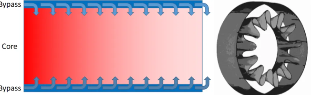
The possibility for different mixers to have very different configurations, see Figure 1, and thereby individual component characteristics, imposes a need to be able to control the state of the mixer within the gas turbine performance code if accurate and detailed modelling of various mixer designs are to be performed. To do so, control and residual variables should be incorporated into the mixer module in the performance code. Different sets of these variables may be chosen depending on what data is available when tuning the model to a physical or simulated application.
Figure 1 Mixer configurations. To the left, principle sketch of an afterburner liner where the bypass cooling flow enters through the multiple holes in the liner. To the right an arbitrarily lobed
mixer design.
Multiple papers has been produced where mixer performance of a specific mixer design is measured [4-5]. A paper from NASA presents an investigation and comparison of 44 different mixer designs [6] in order to find the influences from various geometries on the mixer performance. Other papers focus on 3D simulations of the mixer performance by means of CFD at different operating conditions [3, 8] to get a better understanding of the physical flow field for a specific design. In [7], a study is performed to bridge the gap between experimental investigations of mixer designs and numerical simulations of the flow field. Papers on modelling mixers in 1D simulation codes are in general published in books, program manuals and theory guides [2, 9-10] and only the method chosen by the authors are then presented.
Diagnostics of gas turbines can be classified as either physics based, data driven or a fusion of the two where the classical approach is the Gas Path Analysis, GPA, developed by Urban [11] in the early seventies, where shifts in measurements are correlated to a certain component degradation. The early implementations used linear correlations for fault detection and the method has since been developed to handle non-linear behavior [12]. Other physics based methods make use of Kalman filters [13] to compare actual and estimated outcome from a gas turbine model as a basis for fault detection. Just like the GPA method, the first Kalman filters handled linear problems. More recent methods make use of a nonlinear version named the extended Kalman filter to improve the accuracy for gas turbine diagnostics [14].
Data driven diagnostics make use of various machine learning algorithms that detects faults from anomalies in the data. A common approach is to use a Neural Network, NN, for the detection [15] where the NN is trained to detect a certain kind of fault. Other methods may employ fuzzy logic [16], genetic algorithms [17] or Bayesian belief networks [18] depending on the type of problem to be solved. Combining the physics based and data driven methods may further enhance the diagnostic capability [19]. To the authors’ knowledge, no work on diagnostics on gas turbine mixers has been published. Two diagnostic routines, one based on regression and one on a NN approach, has been developed and evaluated for the detection of an afterburner liner burn-through. An in-house performance code [20] has been modified to include a mixer module and an
engine model mimicking a GE-F414-400 has been created based upon open access data [21]. This model form the basis of all data within this paper.
2.0 MIXER MODELLING
When mixing two streams of different temperatures, a potential thrust gain will occur when comparing the thrust from the mixed fluid to the sum of the thrust from the unmixed streams if they were to ideally expand to ambient conditions. The magnitude of the gain is highly dependent on the bypass ratio, BPR, temperature and pressure differences between the streams. When modelling a mixer with optimal performance, the mass flow, energy and momentum continuity should remain constant between inlets and outlet. This may be sufficient in low fidelity studies but as soon as more accuracy is required, the losses need to be incorporated in some way.
A common approach to incorporate the losses is the mixer efficiency factor that is defined as the actual thrust gain versus the potential thrust gain from an ideal mixing. This is a fairly convenient method since the performance of the mixer is then only dependent of a single parameter. There are however a few drawbacks with this method if a simulation model of a mixer should be tuned to measurement data. When calculating the ideal thrust, an ideal expansion is assumed which makes the thrust a function of the mass flow and velocity. The velocity may be calculated according to Equation 1, assuming a perfect gas.
𝑉 2 ∙ 𝑇 ∙ 𝑅 ∙ 𝛾
𝛾 1∙ 1
𝑝
𝑃 … ( 1 )
Videal is the velocity after an ideal expansion, T is the total temperature, R is the gas
constant, γ is the ratio of specific heats, pamb is the ambient static pressure and P is the
total pressure. The subscript m stands for mixed properties. When the thrust is reduced by the efficiency factor, the ideal velocity is no longer valid and a new, slightly lower, velocity is instead used as input for the calculation back to the total states. Equation 1 is then rearranged to solve for total pressure. This cause a discontinuity where the total pressure out of the mixer is based on a fractional mixing with losses while the total temperature is based on complete mixing. Due to this it is not possible to tune both the pressure and temperature in the mixed state to measurement data. The mixer efficiency as defined above is however often a suitable variable to use when comparing the performance of different mixer designs. Another issue that arises in the special case of two streams of equal total states is that there is no potential thrust gain and therefore, no losses can be modelled.
A method that overcomes these problems uses input stream momentum scaling factors. These are applied to the incoming streams to scale down the incoming momentum before an ideal mixing is calculated. This means that there are now two (or more if more than two input streams are mixed) coefficients that can be used for tuning which will affect both the mixed total pressure and temperature. The downside with this method is that it requires more knowledge by the user about the losses for each stream. The implementation of the scaling factors can be seen in equation 2 where p is static pressure,
A is area, V is velocity, 𝑚 is the mass flow and Msc is the momentum scaling factor. The subscripts 15, 56 and 6 stands for bypass, core and mixed state according to the station numbering that is shown in Figure 3 later in the paper.
𝑝 ∙ 𝐴 𝑉 ∙ 𝑚 𝑀𝑠𝑐 𝑝 ∙ 𝐴 𝑉 ∙ 𝑚
𝑀𝑠𝑐 𝑝 ∙ 𝐴 𝑉 ∙ 𝑚 … ( 2 )
The final method is the multiple stream approach where there are three outlet streams out of the mixer, one fully mixed stream and two non-mixed that goes directly from the inlets, see Figure 2. To use this principle, the user must specify the mass flow fraction of each input stream that should be mixed. The fact that there are three outlet streams from this type of modelling may be either an advantage or disadvantage depending on the purpose of the simulation. The disadvantage may arise at downstream components in the performance simulations that need to be modelled in such a way that it can handle multiple input streams, thus requiring a more complex performance code. It must also be able to cope with the numerical issues that might arise if a complete mixing is required since the mass flow of the unmixed outlet streams then will go to zero. The main
advantage is if the results should be used for analysis where surface temperatures are of interest, such as infrared signature analyses.
Figure 2 Multiple stream mixer principle
The mixer model strategy employed in the EVA gas turbine performance code is with the momentum scaling factors since it gives the user the ability to simulate arbitrary mixer designs without having to deal with multiple streams for the downstream components.
3.0 GAS TURBINE MODEL
The gas turbine model used for the diagnostic method development is a low bypass mixed turbofan in the thrust class of a GE-F414. The model is developed from data available in open literature and is simplified without any recirculating cooling flow, customer bleed air or shaft power extraction. In Figure 3 a schematic overview of the gas turbine can be seen.
Figure 3 Gas turbine model schematic and station numbering
The gas turbine model is created in the in-house gas turbine performance code EVA, which can be used when simulating any kind of gas turbine configuration by building it through component blocks. The mixer model employed in the EVA code is of the momentum scaling type previously described to give the user enough control to tune the mixer component characteristics to test data. Functions has been built in to match an arbitrary mixer inlet pressure ratio, either total or static, or tune it to a certain input stream Mach number, depending on what test data is available.
4.0 MIXER DIAGNOSTICS
When a burn-through of the afterburner liner is present, the flow resistance through the bypass duct is reduced and the engine will operate at a higher BPR for a fixed core speed and exhaust nozzle setting. Due to the higher BPR, the fan rotational speed will increase, causing a shift in the pressure ratio between P21 and P56. It is this shift in pressure ratio that may be detected and correlated to a specific burn-through area.
Since the changes in gas path measurements are very small in case of a burn-through, a repeatable operating condition is important. The diagnostics is therefore intended to be performed during the startup check of the gas turbine while it operates at idle power setting. During this operation, the gas turbine operates at quasi steady state thermal conditions.
An issue that arise during idle condition is the relatively low pressures in comparison with the measurement uncertainties. Measurement sensors have an absolute and a relative uncertainty and, at small pressures, the absolute term may be significant. Another issue is related to the digital control systems used in modern gas turbines where the analog measurements are converted to a digital quantity. Depending on the digital resolution and how the conversion is performed, additional uncertainties are introduced in the measurement. It may therefore be problematic to perform diagnostics from a single
operating point at idle conditions, especially when the magnitude of the numerical deviation sought after is equivalent to the sensor noise. It may also be problematic to run the gas turbine to such an exact state that data between startups can be directly compared. To overcome these issues, a diagnostic system which is not dependent on an exact operating condition is developed to identify a burn-through of the afterburner liner. The diagnostic routine will vary the outlet nozzle area while keeping a specific core speed to get a number of data points at steady state conditions. From the pressure ratio P21 over P56 versus the outlet area A8, a regression analysis is performed to get a trend line. The vertical position of this trend line is then compared to the previous start of the gas turbine to determine if any burn-through has occurred during the last flight. If no burn-through is detected when the test is performed, that data is used to represent a healthy mixer in the next test. By this self-tuning process, effects from gradual degradation of the gas turbine rotating components should be damped.
Two different methods for diagnosing the mixer is compared, one method where an ordinary regression analysis is used and another method using a Neural Network to quantify the damage.
4.1 Data acquisition
All data for this paper is acquired from simulations with the EVA software and the low bypass turbofan model previously described. The ambient conditions for all simulations has been Sea Level Static (SLS) conditions at ISA0 and at a constant core speed of 12000 rpm, representing idle conditions. For sweeps in outlet nozzle area, A8 is varied from 40% to 100% of the nominal design point area in steps of 5%. When simulating a burn-through of the liner, hereafter denoted as a damaged mixer, the bypass input stream momentum scaling factor is increased to represent the lower flow resistance from the afterburner liner.
For the development of the diagnostic methodology, simulations were first performed at idle conditions with a fixed core speed N2 at various A8 settings with a fixed mixer static pressure ratio of unity to get data for a healthy configuration. It is here assumed that the mixer pressure ratio is one for the healthy mixer. For the damaged mixer, the static pressure ratio is not known. It was therefore assumed that the low pressure turbine (LPT) exit Mach number remains constant at a specific core speed and A8 setting, even if the mixer is damaged. This is not entirely true since the LPT exit Mach number is a function of the pressure ratio of the LPT rather than the core speed. The deviation is however negligible for the diagnostic method employed. By making this assumption, the pressure ratio over the mixer can be tuned to match the desired LPT exit Mach number and thereby simulate data for a damaged mixer.
To correlate the burn-through area to a specific shift in bypass momentum scaling factor, simulations with a constant bypass mass flow was performed. This was simulated by tuning the fan mass flow and bypass ratio to a specific target value while keeping the outlet nozzle area A8 constant at the reference condition. For these simulations, the mixer was not controlled in any way since the operating point was determined from the upstream conditions. While doing so, a sweep in bypass momentum scaling factor was performed to get a range of pressure ratios over the mixer as a function of the scaling factor, which could then be used for correlating it to the burn-through area.
4.2 Measurement noise
All physical sensors are in one way or another affected by measurement noise from either variations in the physical field that is being measured and/or uncertainties in the measurement system. If not accounted for, this noise may cause significant deviations from actual results. To investigate the possibility for the methods to detect a burn-through at noisy conditions, a Monte Carlo simulation has been performed where noise according to Table 1 has been injected.
Table 1 Measurement noise and distribution
Measurement Tolerance Distribution
P21 0.25% Normal 3σ
P56 0.25% Normal 3σ
N2 0.05% Normal 3σ
Apart from the sensors in Table 1, there will be measurement uncertainties in the measurement of the nozzle throat area A8. This area is usually calculated from the hydraulic, or in some cases fueldraulic, cylinder position that controls the variable nozzle setting. It is assumed that once the piston reached the position for a certain A8, it is not moved during the data sampling, thus keeping a constant A8. If uncertainties in the cylinder position should cause the sought after A8 be biased from the actual A8, it is assumed to be of negligible influence on the final results since the change in pressure ratio due to a biased A8 is very small. Due to this, disturbances in A8 is not taken into account.
4.3 Regression diagnostic method
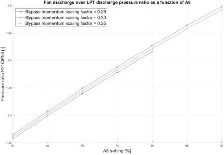
From the simulated data for both healthy and degraded configurations, the pressure ratio P21QP56 is plotted against the relative A8 settings. In Figure 4 plots for both nominal as well as increase and decrease of the bypass momentum scaling factor is shown. Note that the changes in bypass momentum scaling factors are magnitudes larger than what could be expected due to a burn-through. The reason for this is for improved visualization of the diagnostic method. Also note that the curve for bypass momentum scaling factor 0.35 only goes to 80% A8. Opening A8 further while keeping the core speed constant causes supersonic flow in the bypass duct, which is not a feasible operating condition.
Figure 4 P21 over P56 for a sweep in A8 and constant core speed
In Figure 4 a trend of vertical displacement of the curves in the presence of mixer degradations can clearly be seen. It is this displacement that lays the foundation of the correlation between the bypass momentum scaling factor and the burn-through area. If the curve is shifted downwards from the healthy condition, it implies that the fan discharge pressure has decreased, and subsequently lowered the fan speed, due to the smaller flow resistance over the afterburner liner. From the curve for the healthy mixer, a third degree polynomial is fitted with the form in Equation 3.
𝑓 𝑥 𝑐 ∙ 𝑥 𝑐 ∙ 𝑥 𝑐 ∙ 𝑥 𝑚 … ( 3 )
A similar curve fit is then performed for the cases with a degraded mixer where the coefficients c1 to c3 from the healthy condition is used as polynomial coefficients. In this
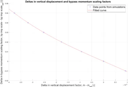
deviation in m and bypass momentum scaling factor is created, which is shown in Figure 5. The reference state refers to the healthy configuration and is used to scale the curve to reduce the uncertainties for small deviations. This is also the rationale for performing it for the upcoming curve fits.
Figure 5 Deltas in bypass momentum scaling and vertical displacement factor
When the data from Figure 4 and Figure 5 is combined, a change in the bypass momentum scaling factor can be derived from the change in P21QP56. The next step is to correlate the change bypass momentum scaling factor to a specific burn-through area to quantify the damage. This correlation is derived from the relationship between mass flow and pressure drop over an orifice in a pipe, which can be seen in Equation 4 from [22].
𝑚 𝐶
1 𝛽 ∙ 𝜀 ∙ 𝜋
4∙ 𝑑 ∙ 2 ∙ 𝜌 ∙ ∆𝑃 …( 4 )
In Equation 4, 𝑚 is the mass flow, 𝐶 is the discharge coefficient, 𝛽 is the diameter ratio of the orifice to the pipe diameter, 𝜀 is the expansibility factor, 𝑑 is the orifice diameter, 𝜌 is the density and Δ𝑃 is the pressure drop over the orifice. The expansibility factor is for pressure ratios greater than 0.75 over the orifice defined according to Equation 5.
𝜀 1 0.351 0.256 ∙ 𝛽 0.93 ∙ 𝛽 ∙ 1 𝑃
𝑃 …( 5 )
𝛾 is the ratio of specific heats and the subscripts 15 and 6 is according to the station numbering. Since the diagnostic routine is only interested in the change in area between two states, and the data for determining the burn-through area is performed at the same mass flow, Equation 4 can be rewritten as follows:
𝐶 1 𝛽 ∙ 𝜀 ∙𝜋 4∙ 𝑑 ∙ 2 ∙ 𝜌 ∙ Δ𝑃 𝐶 1 𝛽 ∙ 𝜀 ∙𝜋 4∙ 𝑑 ∙ 2 ∙ 𝜌 ∙ Δ𝑃 … ( 6 )
The subscripts deg and ref here refers to a degraded, or damaged, mixer and the healthy reference condition. It is obvious that a number of estimations of the afterburner liner geometry need to be undertaken if the geometry is not fully known. For this study, photographs openly available in the public domain of the GE-414-400 gas turbine has been studied as basis of the geometrical estimations. In Equation 6, the term for the diameter squared is replaced by the area and all constants are removed on both sides. An assumption is made that the change in density and discharge coefficient is insignificant
for the different levels of mixer degradation. Rewriting Equation 6 to solve for the delta area yields Equation 7.
Δ𝐴 𝜀 ∙ Δ𝑃
1 𝛽 𝜀 ∙
Δ𝑃
1 𝛽 … ( 7 )
Since the diameter ratio 𝛽 is a function of the original geometry and Δ𝐴, Equation 7 is solved iteratively where 𝛽 is continuously updated with the new area until convergence. The correlation between the bypass scaling factor and the burn-through area can then be seen in Figure 6.
Figure 6 Correlation between change in scaling factor and burn through area
By combining the results from the regression analyses, a correlation between change in the P21QP56 pressure ratio and a burn-through of the afterburner liner is obtained. Before the data is inputted into the regression analysis it is averaged, as seen in Equation 8, for each A8 setting to reduce the impact of the measurement noise. Another choice of averaging is to calculate the pressure ratios first and then perform the averaging. No noticeable change in accuracy of the diagnostic results is noted between the two methods.
𝑃21𝑄𝑃56 𝑃21
𝑃56 … ( 8 )
4.4 Neural Network diagnostic method
The second method consist of a Neural Network (NN) approach where the pressure ratio from both a degraded and a healthy mixer together with the A8 setting is inputted to the NN for training. Averaging of the input data is performed according to Equation 8. When the NN is trained and an area estimate shall be determined, the degraded data is from the last collected samples while the reference is from the last known healthy data collection. The NN will then produce an area estimate for each A8 setting. These estimates will then be averaged to reduce the uncertainties.
Figure 7 Neural Network configuration
A feedforward NN with 10 hidden nodes according to Figure 7 is trained with the Levenberg-Marquardt algorithm. When training the network, 50% of the data has been used for training and the remaining 50% for validation.
4.5 Sensitivity analysis
A sensitivity study is performed to find the number of A8 settings required to get a good enough curve fit from for the regression diagnostic method. 13 different A8 settings with an area increment of ±5% from the reference setting are simulated. Different combinations of the various A8 settings, according to Table 2, are tested with the regression algorithm to determine how many settings that need to be used before a degradation in the calculated result can be noted. The cells marked with an X show the actual A8 settings used for the regression method and the specific number of settings are shown in the left column.
Table 2 A8 settings used for regression diagnostic sensitivity study
A8 area 40 % 45 % 50 % 55 % 60 % 65 % 70 % 75 % 80 % 85 % 90 % 95 % 10 0% 2 X X 3 X X X 4 X X X X 5 X X X X X 6 X X X X X X 7 X X X X X X X 8 X X X X X X X X 9 X X X X X X X X X 10 X X X X X X X X X X 11 X X X X X X X X X X X 12 X X X X X X X X X X X X 13 X X X X X X X X X X X X X
Note that the sensitivity analysis is only presented for the regression analysis. This is because the accuracy of the regression model does not seem to increase at a certain stage when more A8 settings are added, a behavior that is not observed for the NN approach.
5.0 RESULTS AND DISCUSSION
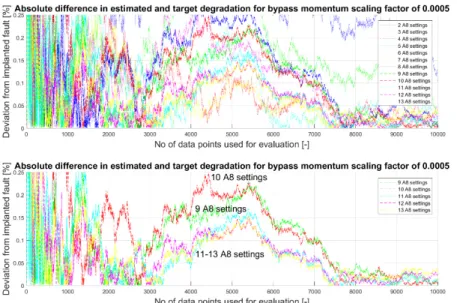
Results from the sensitivity study to find the required number of A8 settings without degrading the final results can be seen in Figure 8. In the upper part of the figure, curves from all combinations of A8 settings are shown while the lower part only contains the settings that seemed relevant to consider after a first visual inspection. Note that the figure is only for a specific implanted degradation, the same plots has been created for other levels of degradation to verify the results. It can be seen that the accuracy does not degrade noticeably when going down to 11 A8 settings while there is a degradation in accuracy when using 10 settings. The choice was then to use 11 settings for A8 when running the regression analysis.
Figure 8 Changes in degradation for various number of A8 settings used for the regression method.
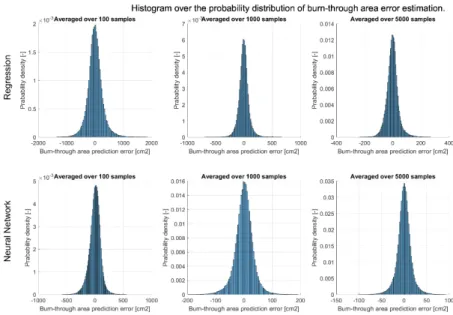
The operating conditions when running the regression and NN methods are at sea level static, SLS, ISA0 and a core speed of 12000 rpm. Histograms of the burn-through area error estimation from the methods when using 100, 1000 and 5000 samples for each A8 setting can be seen in Figure 9. Note that the data in the histograms represent various levels of mixer degradations where the largest deviations come from cases with extremely large burn-through areas. The deviations from more moderate levels of burn-through areas, in the vicinity of a few square centimeters, is shown in Figure 10 together with the time it would take to collect the required data at a sample frequency of 100Hz. Note that the difference in data collection time between the regression and NN methods is due to the two more A8 settings for the NN. The data collection time also includes a two second delay between each A8 setting to allow for the gas turbine to reach the new operating condition.
It is also worth noticing that in Figure 8, an increase in the error estimation is present between 3000 and 7500 samples, a behavior that is not seen in Figure 9. In Figure 8 it is caused by the noise and it will be different every time new noise is added while the results in Figure 9 is averaged over multiple sets of input noise.
Figure 9 Histogram over burn-through area estimations
Figure 10 Sigma 1 levels of moderate burn-through areas and data collection time It is clear that the NN method outperforms the regression method and is therefore the preferred choice. This is mainly due to the post averaging performed by the NN results. If the results are compared before this averaging, both methods produce very similar uncertainties.
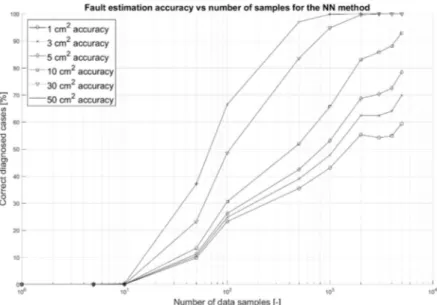
In Figure 11, the amount of correctly diagnosed cases are plotted as a function of number of data samples used for three different accuracies. It is quite clear from the chart that a burn-through of only a few centimeters will be very hard to diagnose without getting a significant number of false positives with the dataset used for this study. In order to reduce the false positives to below 1% and keeping the data collection time within a reasonable time for a startup check, the smallest burn-through area possible to detect is in the magnitude of 40-50 cm2.
Figure 11 Fault estimation accuracy for various number of data samples
6.0 CONCLUSIONS
A study regarding diagnostics of an afterburner liner burn-through has been performed that highlights the possibilities and limitations of a regression and a NN approach. It has been showed that it is hard to detect realistic burn-through area by measuring the small shifts in gas path parameters since it will drown in the measurement noise and uncertainties. Burn-through areas in the magnitude of a few square centimeters should be possible to detect given that enough data is available to filter through the noise in a satisfactory manner, the problem is then the time it takes to collect the data. If the data collection cannot be performed during the time of a regular startup check, it would imply that additional time at idle is required, thereby diminishing the potential gain of implementing such a system. It would then be more convenient to perform visual inspections instead, which is the normal procedure to date.
If the diagnostic system are to be used, there could be certain ways of enhancing it. One way could be to also incorporate the shift in spool speed ratios, which should show a similar behavior as the pressure ratio investigated. Another addition could be to use operational data between the checks. For example, if the system detects what it considers to be a burn-through, it could go back, looking at the usage of the afterburner since the last known healthy state. If the afterburner has not been used since then, the likelihood of it being a burn-through is fairly low. Through this the number of false positives could be decreased.
Regarding the mixer modelling, the choice of modelling strategy is entirely dependent on the purpose of the model. To perform diagnostics as presented herein, the losses of each incoming streams need to be controlled, which could be achieved with either the momentum scaling or multiple stream method. These methods also give the user better possibilities to tune the mixer component characteristics to test data. The model must also be able to simulate and tune the mixer inlet streams to an arbitrary pressure ratio.
ACKNOWLEDGMENTS
The authors gratefully acknowledge the Swedish Research Foundation, KKS, for the financial support.
REFERENCES
[1] T.H. FROST, “Practical Bypass Mixing Systems for Fan Jet Aero Engines”, The
Aeronautical Quarterly, vol. 17, issue 2, pp. 141-160, May 1966.
[2] NATO RTO, “Performance Prediction and Simulation of Gas Turbine Engine
Operation”, RTO-TR-044, 2002.
[3] V.M. BELOVICH, M. SAMIMY, “Mixing Processes in a Coaxial Geometry
with a Central Lobed Mixer-Nozzle”, AIAA Journal, Vol. 35, No. 5, pp.
838-841, May 1997.
[4] S.C.M. YU, J.H. YEO, J.K.L. TEH, “Velocity measurements Downstream of a
Lobed-Forced Mixer with Different Trailing-Edge Configurations”, Journal of
Propulsion and Power, vol. 11, no. 1, pp. 87-97, January-February 1995. [5] H. KOZLOWSKI, M. LARKIN, “Energy Efficient Engine Exhaust Mixer
Model Technology”, NASA Report, NASA-CR-165459, June 1981.
[6] Z. LEI, J. GONG, Y. ZHANG, S. SU, C. HU, “Numerical Research on the
Mixing Mechanism of Lobed Mixer With New De-Swirling Structure”,
Proceedings of ASME Turbo Expo, GT2016-58120, Seoul, South Korea, 2016. [7] M. LECOQ, N. GRECH, P.K. ZACHOS, V. PACHIDIS, “Probabilistic and
Numerical Modelling of a Lobed Mixer at Windmilling Conditions”,
Proceedings of ASME Turbo Expo, GT2013-94366, San Antonio, Texas, USA, June 2013.
[8] B.H. ANDERSON, L.A. POVINELLI, ” Factors Which Influence The Behavior
of Turbofan Forced Mixer Nozzles” NASA Technical Report,
NASA-TM-81668, January 1981.
[9] P. WALSH, P. FLETCHER, “Gas Turbine Performance”, Blackwell, 2nd Ed, 2004
[10] GASTURB, “Design and Off-Design Performance of Gas Turbines”, User Manual.
[11] L. A. URBAN, “Gas Path Analysis Applied to Turbine Engine Condition
Monitoring”, AIAA-72-1082, 1972.
[12] Y. G. LI, “Gas Turbine Performance and Health Status Estimation Using
Adaptive Gas Path Analysis”, Journal of Engineering for Gas Turbines and
Power, vol. 132, pp. 1-9, April 2010.
[13] R. E. KALMAN, “A New Approach to Linear Filtering and Prediction
Problems”, Journal of basic engineering, vol. 82, pp. 35-45, 1960.
[14] F. LU, H. JU, J. HUANG, “An improved extended Kalman filter with inequality
constraints for gas turbine engine health monitoring”, Aerospace Science and
Technology, vol. 58, pp. 36-47, 2016.
[15] R. BETTOCCHI, M. PINELLI, P. R. SPINA, M. VENTURINI, “Artificial
Intelligence for the Diagnostics of Gas Turbines—Part I: Neural Network Approach”, Journal of Engineering for Gas Turbines and Power, vol. 129, pp.
711-719, 2006.
[16] L. MARINAI, “Gas-path diagnostics and prognostics for aero-engines using
fuzzy logic and time series analysis”, PhD Thesis, Cranfield University, 2004.
[17] Y. G. LI, M. F. A. GHAFIR, L. WANG, R. SINGH, K. HUANG, X. FENG, “Nonlinear Multiple Points Gas Turbine Off-Design Performance Adaptation
Using a Genetic Algorithm”, Journal of Engineering for Gas Turbines and
Power, vol. 133, pp. 071701, 2011.
[18] C. ROMESSIS, K. MATHIOUDAKIS, “Bayesian Network Approach for Gas
Path Fault Diagnosis”, Journal of Engineering for Gas Turbines and Power, vol.
128, pp. 64-72, 2006.
[19] R. SINGH, “Advances and Opportunities in Gas Path Diagnostics”, 15th International Symposium on Air Breathing Engines, ISABE-2003-1008, Cleveland, OH, USA, August - September 2003.
[20] K.G. KYPRIANIDIS, “An Approach to Multi-Disciplinary Aero Engine
Conceptual Design”, 23rd International Symposium on Air Breathing Engines,
ISABE-2017-22661, Manchester, UK, September 2017.
[21] B. GUNSTON, “Jane's Aero-Engines”, Jane's Information Group Limited, Issue 10, Surrey, UK, 2001.
[22] ISO 5167-1:2003, “Measurement of Fluid by Means of Pressure Differential