Marginal costs for road maintenance and
operation - a cost function approach
Mattias Haraldsson
September 3, 2007
1
Introduction
In order to fulfil the objectives for the road transport sector, large amounts of money are spent on operation and maintenance measures to keep the
road network functioning. In 2004 Swedish Road Administration (SRA)
expenditures summed to 15 billion (SRA, 2005) SEK1. Of these expenditures
23 percent were generated by operation and 22 percent by maintenance. At present, operation and maintenance measures are financed through the fiscal system although economic optimality conditions state that the wear and tear of vehicles should be priced at marginal cost. However, reliable marginal cost assessments have hitherto not been easily found, primarily due to lack of adequate data. The purpose of this paper is to estimate a set of maintenance and operation marginal costs using data on a low level of aggregation. We also test if marginal cost equals average cost.
According to the definition used by SRA, operation activities are “services to keep the road system functioning, and which result in effects and economic values of a short-term and immediately active nature that last for less than one year.” Maintenance measures on the other hand are defined as “services to preserve or restore the desired properties of the road system, and which result in effects and economic values that last for longer than one year” (Thomas, 2004).
For this study a new data set has been compiled, comprising observed maintenance and operation costs at different levels of detail, vehicle kilo-metres, road categories and pavement types for the whole Swedish national
road network, for the period 1998-2002. Since Sweden covers different climate zones (e.g. polar, semi arid and tempered) the results drawn from an analysis of this data should be fairly general and possible to apply in a variety of ge-ographical contexts. We estimate cost functions where vehicle kilometres is the independent variable of main interest. This approach has not been widely applied in an international context due to its data requirements (Bruzelius, 2004). To our knowledge, few econometric studies based on observational
data have been made, particularly in the road traffic sector.2 International
studies with econometric estimation of road cost functions include Herry and Sedlacek (2002) and Schreyer et al. (2002). A recent study by Link (2006) provides marginal cost and cost elasticities for pavement renewal on German motorways. The costs for different measures are not observed but computed in retrospect, based on rather detailed knowledge about used factor quanti-ties. Cost elasticity is found to be in the interval 0.05 − 1.17 and increases with traffic intensity. The magnitude of the cost elasticity is reported to correspond with earlier studies where it has been estimated to be 0.10 − 1.07. For the railway sector cost functions with observed costs and traffic are es-timated by e.g. Gaudry and Quinet (2003), Johansson and Nilsson (2004) and Andersson (2007).
Thanks to the properties and quality of the database used in this study, we avoid the difficult task of creating a synthetic data from expert assessments or other more or less well motivated assumptions. By means of an analysis that is straightforward in a theoretical as well as methodological sense, we hope to make a substantial contribution to a field that still lacks important empirical results.
Except from total operation and winter operation, that are both found to fixed cost activities, we find short run elasticities in the range 0.25-0.60. We also find that the impact from an additional vehicle is generally mani-fested in extra maintenance and operation costs, not only while the vehicle is using the road, but later on as well. The implication of this is that one has to separate between short and long run cost elasticities and short and long run marginal costs. Point estimates of long run cost elasticities are
2SRA has earlier published marginal cost estimates (Olofsson et al., 2003). These
are, however, based on expert assessments of costs. They first compute costs based on expert assessments of the relationship between passenger car traffic and costs. Then they estimate cost functions now assuming trucks solely to be the cost driving vehicle type. Critical comments on the way the data is generated have also been made by Jansson (2006).
generally (except for gravel road maintenance) higher than one, indicating that marginal costs cover average costs. For total maintenance we have a short run MC of 0.22 SEK/HGV kilometer and a long run MC of 1.34-1.41 SEK/HGV km. Looking at the the corresponding numbers for paved roads, we find these to be 0.16-0.17 and 0.59-0.61 SEK/HGV km. For gravel roads they are 0.56-0.58 and 1.58-1.61 SEK/HGV km. The short run marginal cost for paved road operation is practically zero and the long run marginal cost is 0.01 SEK/vehicle km. For gravel roads the short and long run MC:s are 0.21 and 0.56 SEK/vehicle km.
The paper is organized in the following way. The next section is devoted to the data material where we define and describe the various costs and vari-ables containing information about traffic and the road network. Thereafter, we introduce the reader to the cost function that is used. The fourth section contains results from the estimation and derived marginal cost measures. Finally the paper is closed with a discussion and conclusions.
2
Data
The data set is created by combining two databases from SRA. Cost measures from their business system VERA are matched to traffic and road network
in-formation extracted from a national road register, “V¨agdatabanken” (VDB).
Both these sources of information have been available for a long time, but are unfortunately stored in separate database systems. The analysis in this paper is thus first and foremost a result of extensive manual data processing performed by the author with support from staff at SRA.
The observational entities are 145 maintenance delivery units (MDU)3,
the smallest geographical areas for which costs, traffic measures and network characteristics are available. Thousands of VERA cost records are manually associated with one of the MDU:s in order to relate operation and main-tenance costs to traffic. Figure 1 shows how the observational units are distributed among the seven regions of SRA. Because of the different sizes of regions as well as MDU:s, the number of MDU:s in each region differs. Together the MDU:s cover all of Sweden. Information for each MDU is (with a few exceptions) available for five years, 1998-2002 resulting in a panel data set. To our knowledge the data set has few counterparts even in an inter-national context. The data contains two major cost categories, Maintenance
costs and Operation costs, which can both be further subdivided.4 For
main-tenance we also have information about the two largest subgroups, Mainte-nance of paved roads and MainteMainte-nance of gravel roads. These measures are defined as “maintenance of the road surface, superstructure and substruc-ture, and its runoff and drainage system” on paved and gravel roads. For operation costs we have information about the three largest subcategories. The purpose of operation of winter roads is to “maintain the passability and safety of the road system in accordance with established winter standards during the winter period”. Paved road operation and Gravel road operation include for each road type: costs for “inspection of the road, handling of any administrative task, clean up, rapid rectifications of sudden defects in the road or its draining system.” Besides the described subcategories, total op-eration and maintenance costs also include a number of minor cost categories that will not be subject to separate analyses. One flaw of our data is that the observational units are pretty large. The preferred observation unit is a link, but data on that level is not available. Another problem is that several of the variables describing the traffic and the road network are constant or close to constant over the years. The small variation in traffic volume be-tween years is due to the fact that traffic is not always measured annually and is thus a kind of measurement error. When it comes to the variables describing the road network, however, little or no variation between years is natural, since radical changes in the road network are rare. There are also costs that cannot be connected to a specific geographical area. Table 1 shows the share of each cost category that, due to accounting principles and limited geographical information, cannot be connected to a specific MDU. In the full sample we see that 21 percent of maintenance costs can not be related to a MDU. The corresponding number for total operation is 13 percent. For the analysis we will use both the full sample and a sub sample in which we have excluded regions where missing costs are found to be larger than acceptable (marked with bold-face figures in the table). The last row of the table shows the percent of missing costs in the sub sample.
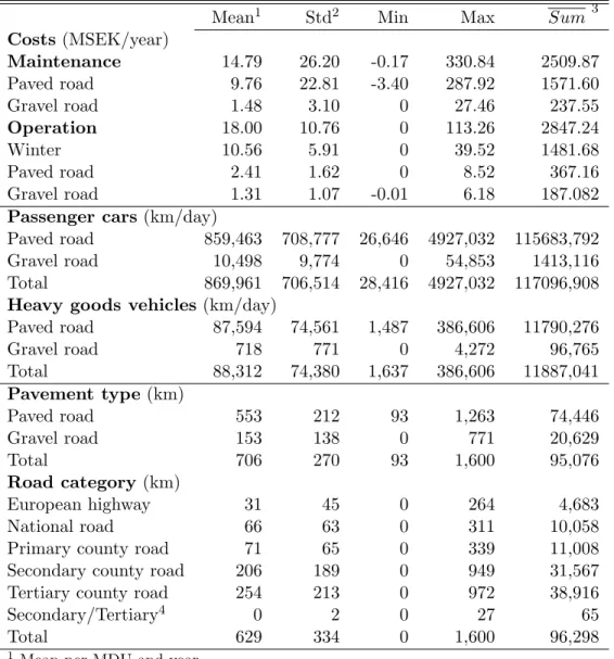
The upper panel of table 2 contains information about the cost data. The second column shows that operation costs are somewhat higher than maintenance costs, and that, on average, 18 MSEK is spent in a MDU each year on operation, where the major part is due to winter operation measures. Almost 15 MSEK is spent annually on maintenance measures in each MDU.
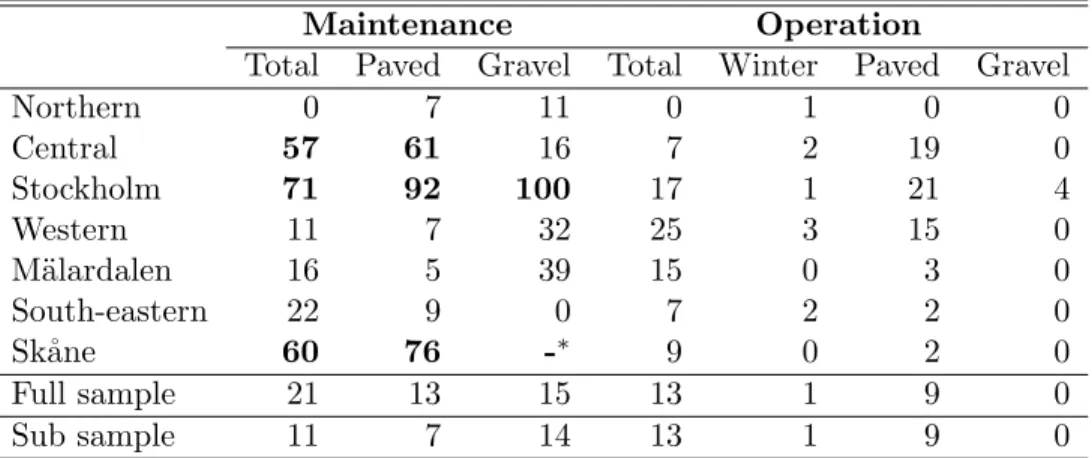
Northern (23) Central (22) Western (38) M¨alardalen (15) Stockholm (8) South-eastern (31) Sk˚ane (8) N
Figure 1: The Swedish Road Administration regions. The number of obser-vational units (MDU:s) in each region is within parentheses.
Table 1: Share of known costs that cannot be related to a specific MDU. Bold-face figures mark data that has been excluded from the analysed sample. The last row shows the shares for the analysed sub samples.
Maintenance Operation
Total Paved Gravel Total Winter Paved Gravel
Northern 0 7 11 0 1 0 0 Central 57 61 16 7 2 19 0 Stockholm 71 92 100 17 1 21 4 Western 11 7 32 25 3 15 0 M¨alardalen 16 5 39 15 0 3 0 South-eastern 22 9 0 7 2 2 0 Sk˚ane 60 76 -∗ 9 0 2 0 Full sample 21 13 15 13 1 9 0 Sub sample 11 7 14 13 1 9 0
∗ Sk˚ane has no recorded costs for gravel road maintenance at all.
Although the logical minimum of each cost is zero, there are a few records with negative “costs”. These can be explained by administrative corrections where erroneous costs are “neutralized” by a negative number. These records are deleted from the data set and are not used in the analysis. The column Sum shows how much is spent in the whole country each year on average. From these measures we see that road maintenance on the national road network costs about 2.5 billion SEK each year and that road operation costs more than 2.8 billion SEK annually.
2.1
Traffic measures
Our data comprises passenger car and heavy goods vehicle (HGV)
kilome-tres5 on different pavement types. The vehicle kilometres data is aggregated
into MDU:s from road links. Descriptive statistics of the different vehicle kilometres are found in the second panel of table 2. The average number of passenger car kilometres each day is 869,961 per MDU and the
correspond-5Vehicle kilometres is based on measured average annual daily traffic (AADT). Some
roads have fixed measurement devices while on other roads mobile equipment is utilized and moved according to a rotating scheme. Data is then adjusted for seasonal varia-tion (Olofsson et al., 2003). Measurement of traffic is done at least every 12 years. These measures are then used without adjustment until a new measure is available (phone con-versation with Dennis Andersson, V¨agverket konsult, 050204).
ing number of HGV kilometres is 88,312, so passenger car traffic is about 10 times higher than HGV traffic. For both vehicle types about one percent of the vehicle kilometers is on gravel roads. We can separate vehicle kilometers on paved and gravel roads but a similar division on different road categories (described in next section) is not possible. Thus we do not know for instance the number of vehicle kilometers traveled on European highways. The Sum column shows how many kilometres are traveled per day in the whole coun-try in an average year. For passenger cars this measure is about 117 million kilometres and for HGV:s about 12 million kilometres. This means that 42.7 billions of passenger car kilometers and 4.3 billions of HGV kilometers are “produced” on the road network each year.
2.2
Network characteristics
The data set also contains information about the kilometres of road in each MDU. We know how these are distributed among several different road cat-egories and pavement types. Road catcat-egories are of great importance in a cost analysis, since they determine the status of a road and are a crucial factor behind operation and maintenance intensity (SRA, 1990). The road categories are: (SRA, 2002).
· European highway: The road is part of an international main road network for Europe.
· National road : The road is part of a network that has been designated by the government as especially important for national welfare.
· Primary county road : Road of national interest.
· Secondary county road : Road of general regional interest.
· Tertiary county road : Road of less importance than secondary county roads.
Descriptive statistics of the road network are found in the lower part of table 2. On average each MDU has 553 km paved roads and 153 km gravel roads. The Sum column shows the kilometres of road with different pavement types and in each road category. This measure is taken as an annual average over the observed years. Logically the total kilometers of road should be the
same irrespective of whether one measures pavement types or road categories. However, some variation is observed due to measurement errors. The national
road network consists of about 95,000-96,000 kilometres of road6, with 74,000
km paved and 20,000 with a gravel surface. A major share of the national road network is classified as county roads. Primary, secondary and tertiary county roads sum up to 81,556 km; about 85 percent of the national road network. The remaining 15 percent belong higher standard and more highly prioritized national roads and European highways.
The kilometres of road in each category are known for the complete MDU network, but not if the network is further divided into paved and gravel roads. Thus, we do not know how the kilometres of paved and gravel roads are distributed among European highways, national roads, and different county roads7.
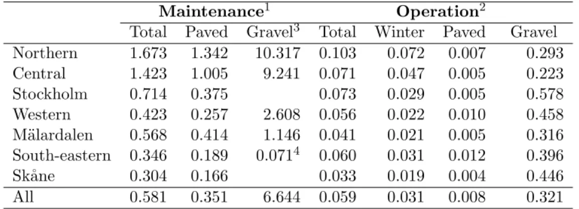
As indicated above, SRA is divided into seven regions, which run oper-ation and maintenance more or less individually. Tables 3 and 4 show two “key statistics”, cost per vehicle kilometre and cost per road kilometre, in order to compare these regions and assess the potential occurrence of geo-graphical patterns. Cost per vehicle km is computed as costs in a specific region divided by the vehicle kilometers on roads where these costs are gen-erated (e.g. costs for paved road maintenance in the North are divided by HGV kilometers on paved roads in the North). Operation costs are divided by total vehicle kilometers. (The reason why different denominators are used is explained below.) Annual cost per road km is computed likewise. We have made adjustments to account for the costs missing in our data (compare with table 1). Unadjusted values can be found in appendix 5.3.
Looking in table 3 at total maintenance cost per HGV kilometre (paved road maintenance follows the same pattern), we can see an interesting pat-tern. The SRA regions are roughly ordered along a north-south dimension (compare with the map in figure 1). It is obvious that the highest per HGV kilometre maintenance costs are found in the north and that this number then falls when we move south. Also, we see that the highest costs for gravel road maintenance are found in the north, although the very low numbers for the South-east probably result from measurement errors. No corresponding geographical patterns for operation costs are visible in the table.
6The annual average total network length is 95,076 km if measured by pavement types
but 96,098 km if measured by road categories.
7It can be suspected though that gravel roads belongs to secondary or tertiary county
Table 2: Descriptive statistics. No adjustments for missing costs. (N=725)
Mean1 Std2 Min Max Sum3
Costs (MSEK/year) Maintenance 14.79 26.20 -0.17 330.84 2509.87 Paved road 9.76 22.81 -3.40 287.92 1571.60 Gravel road 1.48 3.10 0 27.46 237.55 Operation 18.00 10.76 0 113.26 2847.24 Winter 10.56 5.91 0 39.52 1481.68 Paved road 2.41 1.62 0 8.52 367.16 Gravel road 1.31 1.07 -0.01 6.18 187.082
Passenger cars (km/day)
Paved road 859,463 708,777 26,646 4927,032 115683,792
Gravel road 10,498 9,774 0 54,853 1413,116
Total 869,961 706,514 28,416 4927,032 117096,908
Heavy goods vehicles (km/day)
Paved road 87,594 74,561 1,487 386,606 11790,276 Gravel road 718 771 0 4,272 96,765 Total 88,312 74,380 1,637 386,606 11887,041 Pavement type (km) Paved road 553 212 93 1,263 74,446 Gravel road 153 138 0 771 20,629 Total 706 270 93 1,600 95,076 Road category (km) European highway 31 45 0 264 4,683 National road 66 63 0 311 10,058
Primary county road 71 65 0 339 11,008
Secondary county road 206 189 0 949 31,567
Tertiary county road 254 213 0 972 38,916
Secondary/Tertiary4 0 2 0 27 65
Total 629 334 0 1,600 96,298
1 Mean per MDU and year. 2 Standard deviation.
3 Sum over all MDU:s. Annual average 1998-2002.
Table 3: Cost per vehicle km (SEK). An adjustment is made to account for costs that cannot be related to a specific MDU. (N=725)
Maintenance1 Operation2
Total Paved Gravel3 Total Winter Paved Gravel
Northern 1.673 1.342 10.317 0.103 0.072 0.007 0.293 Central 1.423 1.005 9.241 0.071 0.047 0.005 0.223 Stockholm 0.714 0.375 0.073 0.029 0.005 0.578 Western 0.423 0.257 2.608 0.056 0.022 0.010 0.458 M¨alardalen 0.568 0.414 1.146 0.041 0.021 0.005 0.316 South-eastern 0.346 0.189 0.0714 0.060 0.031 0.012 0.396 Sk˚ane 0.304 0.166 0.033 0.019 0.004 0.446 All 0.581 0.351 6.644 0.059 0.031 0.008 0.321 1 Cost per HGV km
2 Cost per vehicle km (HGV:s+passenger cars)
3 N=645. In Stockholm gravel road maintenance costs cannot be related to MDU:s.
Sk˚ane has no recorded costs for gravel road maintenance.
4 The low number in the South-eastern region is probably due to unknown missing
costs in the data.
Table 4: Annual cost per road km (SEK). An adjustment is made to account for costs that cannot be related to a specific MDU. (N=725)
Maintenance Operation
Total Paved Gravel1 Total Winter Paved Gravel
Northern 32,616 38,854 19,248 21,098 14,686 2,005 7,352 Central 45,765 43,259 20,814 24,929 16,424 2,463 7,148 Stockholm 41,741 24,125 60,184 23,887 4,556 2,205 Western 25,625 18,905 3,884 36,835 14,293 7,946 13,063 M¨alardalen 34,937 31,789 2,208 26,428 13,369 3,991 10,926 South-eastern 16,760 10,807 822 28,416 14,432 6,812 8,589 Sk˚ane 18,903 12,142 23,748 14,092 3,418 5,987 All 26,495 20,284 11,375 29,291 15,100 4,788 8,567
1 N=645. In Stockholm gravel road maintenance costs cannot be related to MDU:s.
Sk˚ane has no recorded costs for gravel road maintenance.
2 The low number in the South-eastern region is probably due to unknown missing
Turning now to the cost per road kilometer in table 4, no distinct geo-graphical patterns are discernible. One might dare to say that the north-south pattern is there for paved road maintenance, although not very clear. The two highest numbers are found in the two northernmost regions and the two lowest are found in the southernmost regions. For gravel roads we notice again that the South-eastern region has a value that is lower than plausible. Operation costs per road kilometre seem to vary without any geographical pattern at all.
3
Method
We view the road transport system as an apparatus where various production factors are transformed into a road network with certain properties, and where a certain number of vehicle kilometres are produced. Our approach is to estimate the dual of the production function.
The focus of our interest is the impact of some traffic measures on main-tenance and operation costs. All other things equal, the additional cost of an
extra vehicle km, equivalent standard axels loading8 (ESAL) km or similar
is the marginal cost.
For the continuing work we have to decide which traffic measure to as-sociate with each cost. An attractive approach would be to simultaneously analyse the impact from passenger cars and HGV:s. However, regression analysis of strongly correlated regressors, such as passenger car and HGV kilometres, results in poor precision because of strong multicollinearity. To circumvent this problem Link (2002) uses the ratio between the number of trucks and personal cars. Although this resolves the multicollinearity, a neg-ative consequence, noted by the author, is the problem of how to interpret the parameters. Since such a quotient efficiently removes the quantitative nature of the regressor, roads might get the same ratio even if traffic volumes differ by a large (arbitrary) factor.
In this paper we instead make a priori decisions about which vehicle kilometer variable to use thereby determining the unit of the marginal costs that will be derived. For maintenance models we can base this decision on
8The point of departure of standard axel computation is the so-called fourth power
law of the relation between axel weight and road wear. The number of standard axels associated with a specific vehicle is the sum of the fourth power of each axel weight divided by 104(DOT, 1994).
technical knowledge about the relation between axle loadings and the wear and tear of roads. It is commonly assumed that the need for maintenance is caused by the number of ESAL:s that have passed a road section. This is based on the AASHO-test in the 1960:th, where it was found that road wear and deformation is related to ESAL:s (Johnsson, 2004). The average number of ESAL:s for HGV:s in Sweden is 1.3, while the number of ESAL:s for passenger cars are practically zero (SRA, 2003). This assumption allows us to exclude passenger cars from the maintenance cost functions and focus on
HGV traffic only.9 The resulting marginal costs will be expressed as SEK per
HGV kilometer. When it comes to operation cost functions there is no similar knowledge to rely on but the definition of operation measures provides some guidance. The operation of winter roads is an activity managed according to winter standards, mainly related to road category and total traffic flow. Our choice is therefore to explain these costs by the sum of passenger cars and HGV:s with the resulting marginal cost expressed in SEK per vehicle kilometer. The operation of paved and gravel roads includes road inspection,
administrative issues, clean up and minor repairs. Since it is hard to a
priori relate these activities to a specific type of vehicle, we use the sum of passenger cars and HGV kilometers in this case as well. As a consequence of these choices, total operation cost is also modelled as a function of total vehicle kilometers.
3.1
Model
The road holder is assumed to minimize the operation and maintenance costs necessary to produce a given level of traffic on a certain road standard. The efforts of the road holder can then be expressed as a set of conditional fac-tor demands that can be summarized in a cost function (Varian, 1992). To make things easy we assume that the dominating factor necessary to produce transport is road capital, which is deteriorated by traffic and thus has to be “replaced” to keep the road standard at its desired level. We know that a certain gap between actual and desired level is allowed before any mea-sures are undertaken (SRA, 1990). Such a policy can be explained by lumpy adjustment costs that make instant adjustments inefficient. Although this generates a discrete stream of investments for single roads, it has been shown
9Although passenger cars contributes to pavement deterioration, in particular when
that, at the aggregate level this is a smooth process, well approximated by an autoregressive (AR) model (King and Thomas, 2006). This is the
par-tial adjustment model10 which motivates the inclusion of costs for measures
undertaken earlier in the cost function. Since conditional factor demands are based on certain output levels, traffic should also be included in the cost function. Finally, we include certain other factors that can be assumed to have an influence on maintenance and operation costs as well. We assume that the following formulation makes up a satisfactory approximation of the true cost function:
lnCit= α + αr+ αt+ βClnCit−1+ βQlnQit
+ βQ2(lnQit)2+ βZlnZit+ εit
(1) where C is the cost, Q is vehicle kilometres (defined differently for different costs as discussed above) and Z is a vector describing the road network. This vector contains information about the length of roads belonging to various road categories or with different pavement types. In the former case, Z covers all the national road network. This is used when costs that are generated anywhere in the road network are analysed (total maintenance or operation costs and operation of winter roads). In the second case, the vector describes the total length of paved or gravel roads, a formulation used when pavement specific costs are analysed (maintenance/operation of paved or gravel roads). The row sum over Z is a measure of the relevant road networks length in
a MDU for a specific year. αr are effects specific to each SRA region, αt
are year dummies and εit are random errors. Equation 1 is a simplified cost
function where factor prices have been excluded. We assume factor prices to be constant over all units, allowing us to exclude them from the analysis without interfering with elasticity and marginal cost computations. Between-years variations in prices are accounted for by the year dummies.
As we are using a data set where the units are observed over several years, a natural extension to equation 1 would be individual unobserved effects, in order to improve heterogeneity control. The reason that this approach is not utilized is that our traffic measures, as mentioned above, show little or no between years variation. This feature is an obstacle to panel data estimation
of the parameters of main interest, βQ and βQ2.
10This approach has been used for a long time, motivated by quadratic adjustment costs.
We expect a positive relation between traffic and cost, that is a
posi-tive βQ. Increasing or decreasing return on the other hand, i.e negative or
positive βQ2, is not subject to a priori assumptions. When it comes to the
interpretation of βZ, which expresses the effects on costs from the network
size, it might at first seem clear that this should be positive, i.e. that costs should increase with the kilometre road contained in a MDU. However, con-sider a case where two MDU:s have equal vehicle kilometers. Then, it is not obvious that the MDU with a larger road network has higher maintenance
or operation costs. Thus the sign of βZ is an empirical question.
Using the lag operator11 equation 1 can be rewritten:
(1 − βCL)lnCit = α + αr+ αt+ βQlnQit
+ βQ2(lnQit)2+ βZlnZit+ εit
(2)
where if |βC| < 1 the time series is stationary.12 Rewrite again13:
lnCit= α∗+ α∗r + α ∗ t + 1 1 − βC h βQlnQit+ βQ2(lnQit)2 i + βZ∗lnZit+ ε∗it (3)
For the understanding and interpretation of this model, it interesting to see that this is the limit of the geometric sum:
lnCit = α∗+ α∗r+ α ∗ t + ∞ X j=0 βCjLjhβQlnQit+ βQ2(lnQit)2 i + βZ∗lnZit+ ε∗it (4)
Thus, cost is dependent of the complete history of Q. If |βC| < 1, the
impact from past traffic decreases with time. The closer βC is to zero, the
less important is the history.
11The lag operator L is defined by: x
t−1= Lxt.
12A series are considered covariance stationary if the expected value and variance is
constant over time and if the covariance between two observations depends on the interval between them but not on the time the observations are taken.
13The asterisk (*) implies that the parameters have been transformed by the factor 1
4
Analysis
First a few words about the way we deal with the known missing costs. As noted above, all costs cannot be connected to a MDU and are therefore not included in the data, a problem particularly prominent in some SRA regions (see table 1). As long as such measurement errors are unrelated to our regressors they do not impede consistent estimation (see for instance Greene, 1997), but the validity of such an assumption can of course not be taken for granted. To get an impression of the sensitivity of the estimates to the missing costs, we have estimated all maintenance models both on the full sample and on the sub sample where regions badly struck by this problem
have been excluded. A brief look at the most important coefficients, βC, βQ
and βQ2 reveals that using the full sample or the sub sample is a choice of
little practical importance. We could exclude either but choose to base the discussion of the results on both samples. When showing numbers in the text, intervals illustrate the differences between full and sub samples. As we have seen above, missing costs are a negligible problem for operation so for operation estimations are only made on the full sample. For all types of operation and maintenance measures we adjust for missing costs when average and maintenance costs are computed.
The results of our estimations are found in tables 5 and 6. Since a lagged variable is included in the models, we lose one year (1998) of observations. Two estimation techniques are utilized. The simplest possible is ordinary least squares (OLS) which yields consistent estimates, given that there is no serial correlation in the error terms (Greene, 1997). Durbin-h tests, based on OLS residuals, reveal that this assumption holds for the operation cost models but not for maintenance costs. In the latter case, therefore, we switch
to instrumental variable (IV) regression, using Ct−2 as an instrument. The
downside of this procedure is that one additional year of observations is lost. As shown by equation 1 we assume a potentially non-linear relation
be-tween lnC and lnQ. We thus start by estimating cost functions with (lnQ)2
on the right hand side and then drop the squared variable if its coefficient
is found to be insignificant.14 The final maintenance cost models are
esti-mated without the squared vehicle kilometer term since βQ2 is found to be
insignificant in these three models. The result is a relation between traffic and costs where the cost elasticity is constant at all traffic levels. Overall
model fit is very good in all cases, maintenance as well as operation cost
models, indicated by R2 adjusted values in the range 0.50-0.92.
The coefficient of main interest, βQ is positive, as expected, in all the
maintenance models. In the total maintenance and paved road models this coefficient is highly significant. In the paved road maintenance models it is
significant using the full sample only. We further notice that βC is about
0.83-0.85 for total maintenance costs, while it is lower, 0.72-0.73 and 0.64 for paved and gravel road maintenance costs. Hence, the effect from earlier periods is larger for total maintenance costs than for the subcategories. All
operation cost models have positive and significant βQ. The total and winter
models also have significant and negative βQ2 indicating that costs increase
with traffic but at a decreasing rate. In the models for paved and gravel road operation costs the squared terms are dropped due to insignificance. For all
operation cost models the lag coefficient βC is 0.61-0.62.
In the middle section of the result tables we have the βZcoefficients, which
express how the road network size (and composition) affects costs. These coefficients are never significant in the maintenance cost models. Thus, it does not matter, in terms of costs, whether the traffic is concentrated to few kilometers or distributed on a large network. In the operation cost models there is a mixture of significant and non significant network coefficients, the signs of which shift in an interesting manner. Beginning with the models for total operation and winter operation we see that coefficients are positive
for all road categories but tertiary county roads. Positive signs indicate
that, given the traffic volume (and other factors as well), a more extensive road network increases costs. The negative sign observed for tertiary county roads instead shows costs to be decreasing with the kilometers of roads. This might seem surprising, but can be explained by the fact that too much traffic is concentrated to a few kilometers of road, resulting in substantial needs for operation measures. Negative signs are also observed in the gravel and paved road operation models. Thus, distributing a given amount of traffic on a larger number of road kilometers would reduce costs for gravel and paved road maintenance. That the road network variables vary between different models is due to the fact that some costs are generated on the whole road network while others are generated on paved or gravel roads only. In the former case we describe the network in terms of the kilometers of road in different road categories, while in the second case the kilometers of paved and gravel roads are used.
tem-poral dummies that capture differences between SRA regions and various years. For maintenance, the only significant regional dummies are found in the gravel model. They show (both for the complete sample and the sub sample) that the North and Middle regions have significantly higher costs for gravel road maintenance than the reference region. Looking at the operation cost models, we see that the South east has lower costs for total operation and winter operation measures. Total maintenance costs (sub sample) were significantly higher in 2000 than in 2002. Operation costs were higher in 1999 compared to 2002.
4.1
Elasticities and marginal costs
We use the parameter estimates to derive cost elasticity estimates, i.e the percentage change in cost that results from a one percent change in traffic. We compute two different elasticities, one short run elasticity, which expresses how a change in traffic changes costs in the same year, and one long run elasticity where cost changes in subsequent years are also accounted for. The log linear form of our cost functions enables easy computation of the cost
elasticities as shown in equations 5 and 615. Disregarding dynamic effects,
i.e. conditioning on Cit−1, we get the short run elasticity (impact multiplier):
δlnE(Cit|Cit−1)
δlnQit
= ˆηitSR = βQ+ 2βQ2lnQit (5)
The long run cost elasticity is: δlnE(Cit)
δlnQit
= ˆηitLR = 1 1 − βC
(βQ+ 2βQ2lnQit) (6)
As mentioned above, βC determines the importance of history for present
costs, which is manifested also by the fact that long and short run elasticities
are equal if βC = 0. Variances in the cost elasticity estimates are computed
using the delta method (see for instance Greene, 1997). Knowing elastici-ties to be functions of estimated parameters and knowing the variances for the parameters to be σ2ˆ βQ, σ 2 ˆ βQ2 and σ 2 ˆ
βC and covariances σβˆQβˆQ2, σβˆQβˆC and
σβˆ
Q2βˆC, the variances of the estimated long and short run elasticities are (we
skip the indices i and t for notational simplicity):
T a ble 5 : M a in tenance co st functio n co efficien ts (IV) T otal P a v e d Gra v el F ull sam p le 1 Su b sam p le 2 F ull sam p le 1 Su b sa mp le 2 F ull sam p le 1 Su b sam p le 3 es t t es t t e st t es t t es t t e st t α -0.64 -1.08 -0.26 -0.87 0.63 0.47 1.25 1.18 -0.83 -0.93 -0.70 -1. 09 lnC t− 1 0.83 19.20 0.85 21.10 0.72 7. 79 0. 73 6.02 0.64 7.05 0.64 6.63 lnQ (HGV) 0.27 3. 27 0. 25 3.81 0.36 2 .11 0. 30 1.35 0.26 2.20 0.27 2.09 lnK meur op ea n -0.04 -0.85 -0.04 -1.02 lnK mnati onal 0.02 0.30 0.03 0.44 lnK mpr im a r y 0.03 0.33 0.08 1.22 lnK msecond a r y 0.01 0.08 -0.03 -0.28 lnK mter tiar y 0.03 0.36 0.03 0.43 lnK mpav ed -0.05 -0. 19 0. 02 0.06 lnK mg r a v el -0.12 -0.87 -0. 12 -0. 76 North 0.42 0.95 -0.15 -0.29 0. 96 0. 66 0. 32 0.34 4.46 3.13 4.23 3.21 Ce n tral 0.08 0.19 0. 34 0. 26 4.75 3.24 4.52 3.32 St o ckh olm 0.08 0.14 -1. 99 -1. 49 1.10 1.06 W e st -0.01 -0.03 -0.52 -1.37 -0. 91 -0. 88 -1. 40 -1.57 0.13 0.17 -0.11 -0.22 M¨ al ardal e n 0.17 0.39 -0.38 -0.84 0. 52 0. 38 -0. 07 -0.08 1.20 1.04 0.94 0.95 Sou th eas t 0.44 0.82 0. 60 0. 51 0.25 0.31 2000 0.28 1.44 0.37 2.21 -0. 87 -1. 62 -0. 55 -0.82 0.07 0.17 0.01 0.02 2001 -0.20 -1.02 -0.21 -1.27 0. 01 0. 02 -0. 40 -0.61 -0.05 -0.93 -0.70 -1.09 N 434 320 429 318 435 387 R 2 adj usted 0.83 0.92 0.56 0.50 0.76 0.75 1 Sk ˚ane is the reference region al d umm y an d 2002 is th e reference y ear. 2 Ce n tral, S to ck holm and S k˚ ane ha v e b ee n exclud e d from the sample. Sou th eas t is the re fe re n c e re gi onal du mm y. 3 St o ckh olm an d S k˚ ane ha v e b e en exc lud e d from the sample. Sou th e ast is th e reference re gion al du m m y .
T a ble 6 : Op eratio n co st functio n co efficien ts (OLS) T o tal Win ter P a v ed Gra v el est t est t est t est t α 0.9 7 1.38 1 .04 1 .59 -0.0 3 -0.05 0 .53 1 .18 lnC t− 1 0.6 1 1 6.93 0 .61 18 .11 0.6 1 1 7.27 0 .62 22 .34 lnQ (to tal tr affic) 0.62 3 .75 0 .57 3.5 7 0.41 9 .49 0. 59 1 3.0 1 (l nQ ) 2 -0.02 -2 .26 -0 .02 -2.0 0 lnK meur ope a n 0.1 0 1.75 0 .08 1 .49 lnK mnatio nal 0.1 0 1.51 0 .09 1 .40 lnK mpr im a r y 0.0 6 0.72 0 .05 0 .69 lnK msecond a r y 0.4 0 3.15 0 .38 3 .12 lnK mter tiar y -0.25 -2 .79 -0 .22 -2.6 2 lnK mpav e d -0.07 -0 .79 lnK mg r av el -0.10 -1 .67 Nor th 0.65 1 .34 0.7 0 1.4 9 0.34 0 .87 -0.2 8 -0.74 Cen tra l 0.22 0 .49 0.3 0 0.7 1 0.00 0 .01 -0.6 3 -1.65 Sto ck holm -0.02 -0 .03 -0.2 6 -0.4 8 -0.63 -1 .35 -0.3 1 -0.6 4 W est 0.12 0 .29 0.0 2 0.0 5 0.25 0 .68 -0.4 4 -1.23 M¨ ala rdalen 0.25 0 .55 0.3 3 0.76 0.26 0 .64 -0.3 4 -0.83 Sout h ea st -1.38 -2 .39 -1.3 4 -2.3 9 0.30 0 .80 -0.2 5 -0.6 8 19 99 0.61 2 .58 0.5 5 2.38 0.64 2 .91 0.4 9 2.25 20 00 0.10 0 .44 -0.1 0 -0.4 4 0.25 1 .14 0.3 3 1.56 20 01 0.40 1 .72 0.1 8 0.78 0.32 1 .45 0.2 9 1.34 R 2 adjusted 0.6 5 0 .68 0.6 4 0 .83 Sk ˚ane is the reference region al d umm y an d 2002 is th e ref e rence y ear.
σ2ηˆ LR = h 1 1 − ˆβC i2 σβ2ˆ Q+ 2 h 1 1 − ˆβC ih 2lnQ 1 − ˆβC i σβˆ QβˆQ2 + 2h 1 1 − ˆβC i ˆβQ+ 2 ˆβQ2lnQ (1 − ˆβC)2 σβˆQβˆC + h 2lnQ 1 − ˆβC i2 σβ2ˆ Q2 + 2 h 2lnQ 1 − ˆβC i ˆβQ+ 2 ˆβQ2lnQ (1 − ˆβC)2 σβˆ Q2βˆC + h ˆβQ+ 2 ˆβQ2lnQ (1 − ˆβC)2 i2 σβ2ˆ C (7) ση2ˆ SR = σ 2 ˆ βQ+ (2lnQ) 2σ2 ˆ βQ2 + 4lnQσβˆQβˆQ2 (8)
Multiplying elasticities with the predicted average costs we finally get estimates of the marginal costs. We compute short and long run marginal costs by multiplying the elasticities by average costs:
d
M CSRit = ˆηSRit ACdit (9)
d
M CLRit = ˆηLRit ACdit (10)
where average costs (AC) are computed using the fitted costs divided by the output measure:
d
ACit = bCit/Qit (11)
For policy purposes, the long run marginal cost is probably the most relevant since it expresses what an extra vehicle kilometer means in terms of
extra costs, not only in the present period but also totally.16
An implication of this is that marginal cost pricing generates full cost coverage only if the cost elasticity is equal to or higher than unity (η ≥ 1).
Average elasticities and their t-values are shown in table 7. In a constant
elasticity model the mean elasticity is trivially ˆη and can be obtained directly
from our estimation results in tables 5 and 6. For those two models where
16Our definition of long run marginal costs is maybe a bit unorthodox. Long run costs
are usually meant to express costs should there be no capacity limits or other conditions that are given in the short run. Here, however, long run marginal cost means the sum of all costs, instant or future, that are caused by an extra vehicle kilometre. We motivate this definition by the fact that we use the notion long term elasticity (multiplier) which is standard terminology in time-series regression (see e.g. Greene, 1997).
elasticity is non-constant, we compute the values of equations 6 and 5 at the average of Q.
For total maintenance costs, the short run elasticity is estimated to be 0.25-0.27. For paved roads we find a short run elasticity estimate in the range 0.30-0.36. The gravel road short run elasticity estimate is 0.26-0.27. Turning to the long run elasticity estimates it is interesting to find these to be well above one both for total maintenance costs (1.60-1.64) and for paved road maintenance (1.12-1.20). For gravel roads the long run elasticity estimate is below one, however, 0.71-0.75. One explanation for this might be that other factors, like weather, have a large impact on the condition of gravel roads and that costs for maintenance are thus caused by traffic only to a limited extent.
Turning to operation costs, we see that, for total operation and winter operation measures, elasticity estimates are non-significant. They are also negative, which clearly is not sensible. Therefore, no marginal costs are
computed (they are zero)17. Paved road operation has (significant) short and
long run elasticities estimated at 0.41 and 1.06 respectively. For gravel roads the corresponding numbers are 0.59 and 1.54, which are also significantly different from zero.
The right-hand part of table 7 shows AC and MC. We have computed MC:s based both on the short and long run elasticities. The numbers relevant
for policy purposes are the adjusted values18. We have used predictions of
the average costs and then adjusted these upwards based on our knowledge about missing costs (compare with table 1). Multiplying this value with either of the elasticities results in the adjusted short and long run marginal costs. For total maintenance we have a short run MC of 0.22 SEK/HGV kilometer (same for the full and sub samples) and the long run MC is 1.34-1.41 SEK/HGV km. Looking at the corresponding numbers for paved roads, we find these to be 0.16-0.17 and 0.59-0.61 SEK/HGV km. For gravel roads they are 0.56-0.58 and 1.58-1.61 SEK/HGV km. The short run marginal cost for paved road operation is practically zero and the long run marginal cost is 0.01 SEK/vehicle km. For gravel road operation the short and long run MC:s are 0.21 and 0.56 SEK/vehicle km.
17This is in line with what can be expected. Jansson (1996) claims for instance that
costs for cleaning roads from snow are fixed to a very large extent.
18For gravel road operation we use unadjusted values since no costs are missing in this
T a ble 7: Results -summary . Unadjusted v a lues are comp uted without regar d to kno wn missing costs, while, fo r the a dj usted v a lue s, m is sing costs has b een ta k en in to accou n t. (Cost unit: SEK/KM) Unad ju sted Ad ju sted Cos t Sample T raffi c meas u re ¯ ˆηS R t 1 ¯ ˆηLR t 1 d AC dM CS R dM CLR d AC dM CS R dM CLR Main tenance F ull HG V k m total 0.27 3. 26 1. 60 3.35 0.66 0.18 1.06 0.84 0.22 1.34 Su b HG V k m total 0.25 3. 80 1. 64 3.91 0.76 0.19 1.25 0.85 0.22 1.41 P a v ed road F u ll HGV km pa v e d 0.36 2.10 1.27 2. 24 0.41 0.15 0. 53 0.48 0.17 0.61 Su b HG V k m pa v ed 0.30 1. 34 1. 12 1.45 0.49 0.15 0.55 0.52 0.16 0.59 Gr a v el road F u ll HGV km gra v e l 0.26 2.19 0.71 2. 23 1.88 0.48 1. 34 2.21 0.56 1.58 Su b HG V k m gra v el 0.27 2. 09 0. 75 2.12 1.84 0.50 1.38 2.14 0.58 1.61 Op er at ion 2 F ull V e h ic le km total -0.05 -0. 29 -0. 12 -0.29 0.09 0.10 Win te r 1 F ull V e h ic le km total -0.00 -0. 01 -0. 00 -0.01 0.05 0.05 P a v ed road F u ll V ehi c le km p a v ed 0.41 9.49 1.06 9. 20 0.01 0.00 0. 01 0.01 0.00 0.01 Gr a v el road 3 F ull V e h ic le km gr a v e l 0.59 13. 00 1. 54 15.17 0.36 0.21 0.56 1 ˆη /std 2 No m ar gin al costs are c ompu te d sin c e the e lasticites are far from sign ifican t (an d negativ e). F or th e se mo d e ls, whic h in c lu de a squ ared te rm , th e p res en ted m ean elastic ities are compu te d at th e me an of Q . Th us ¯ ˆη= ˆη ( ¯ Q). 3 No adj ustm en t is nec es sary since all costs are includ ed in th e samp le .
Table 8: Test for whether long run elasticity equals one
Cost Sample η¯ˆLR t∗
Maintenance Full 1.60 1.25
Sub 1.64 1.52
Paved road Full 1.27 0.47
Sub 1.12 0.16
Gravel road Full 0.71 -0.89
Sub 0.75 -0.70
Operation Full
Winter Full
Paved road Full 1.06 0.49
Gravel road Full 1.54 5.34
∗ H
0: ¯ηˆLR= 1
4.1.1 Does MC equal AC?
As discussed above, with marginal cost pricing, the infrastructure is effi-ciently used. In practice though, road holders might not only be interested in efficiency but would like to cover their costs as well (this is the idea of “cost accounting”). This is done by charging AC. Thus, the dilemma is that efficiency and cost coverings are combined only in the special case where
M CLR = AC. This makes it worthwhile to have an extra look at the
elas-ticity estimates. We test whether the long run elasticities are equal to one.
Should this hypothesis hold, M CLR = AC. Table 8 again shows the long
run elasticities, now accompanied by t-values indicating whether or not the point estimates are different from one. As we can see, this is only the case in one instance; gravel road operation costs. In all other cases there is no statistical evidence against the conjecture that M C = AC.
5
Conclusions
In this paper we estimated several cost functions with good result and de-rived estimates of cost elasticities and marginal costs. We do not repeat all the elasticity and marginal cost measures from the preceding section but describe the results in more general terms. We find that costs for operation and maintenance measures increase with traffic intensity, except from total operation and winter operation, which are found to be fixed cost activities.
That the need for roads free from snow is equally large whether there are just a few vehicles using the road or there are plenty of them is quite natural. That the same is true even for the total, can be explained by the fact that winter operation is the dominating sub category.
We have also found that the impact from an additional vehicle is mani-fested in extra maintenance and operation costs, not only when the vehicle uses the road, but later on as well. The implication of this is that one has to separate between short and long run cost elasticities and short and long run marginal costs. We find generally that short run elasticities are in the range 0.25-0.60 for different operation and maintenance measures indicating the share of costs that is covered with a pricing scheme (or taxes) based on short run marginal costs. Point estimates of long run marginal costs, however, are generally higher than average costs (except for gravel road maintenance). Should those using the roads be held accountable for the long run costs that their marginal traffic results in, road holders will need no extra source of financing.
For total maintenance we have a short run MC of 0.22 SEK/HGV kilo-meter and the long run MC is 1.34-1.41 SEK/HGV km. Looking at the the corresponding numbers for paved roads, we find these to be 0.16-0.17 and 0.59-0.61 SEK/HGV km. For gravel roads they are 0.56-0.58 and 1.58-1.61 SEK/HGV km. The short run marginal cost for paved road operation is practically zero and the long run marginal cost is 0.01 SEK/vehicle km. For gravel roads the short and long run MC:s are 0.21 and 0.56 SEK/vehicle km. An interesting result is also the fact that long run equality between marginal and average costs cannot be ruled out.
The analysis in this paper is based on rather strong assumptions about what costs are caused by passenger cars and what are caused by HGV:s. In particular this is the case for road maintenance. To get more robust results several strategies are possible. The first is to extend the data set. With a larger number of observations it would probably be possible to estimate separate elasticities/marginal costs for passenger cars and heavy goods vehi-cles without encountering statistical problems. Another approach is to use a single traffic index for point estimation and then differentiate using other knowledge. In a coming project we plan to analyse how vehicles with differ-ent axle configurations, weight, tyres etc. deteriorate the road pavemdiffer-ent in an experimental setting.
References
Andersson, M. (2007). Fixed effect estimation of marginal railway infrastruc-ture costs in Sweden. Mimeo.
Bruzelius, N. (2004). Measuring the marginal cost of road use - An interna-tional survey. Meddelande 963A, Swedish Nainterna-tional Road and Transport Research Institute.
DOT (1994). The allocation of road track costs 1995/1996. Department of Transport Statistics Directorate.
Gaudry, M. and Quinet, E. (2003). Rail track wear-and-tear costs by traffic class in France. In First conference on railroad industry structure, compe-tition and investment. Institut d’Economie Industrielle.
Greene, W. H. (1997). Econometric Analysis. Prentice Hall, 3:rd edition. Hamermesh, D. S. and Pfann, G. A. (1996). Adjustment costs in factor
demand. Journal of Economic Literature, 34:1264–1292.
Herry, M. and Sedlacek, N. (2002). Road econometrics - Case study motor-ways Austria. Annex A1c Deliverable 10: Infrastructure Cost Case Studies, Unite. Version 1.1.
Jansson, J. O. (1996). Transportekonomi och livsmilj¨o. SNS F¨orlag. In
Swedish.
Jansson, J. O. (2006). Kommentarer till avsnittet om slitage och milj¨o i
“ ¨Oversyn av marginalkostnader inom v¨agtransportsektorn”. In Swedish.
Johansson, P. and Nilsson, J.-E. (2004). An economic analysis of track main-tenance costs. Transport Policy, 11:277–286.
Johnsson, R. (2004). The cost of relying on the wrong power - Road wear and the importance of the fourth power rule (tp446). Transport Policy, 11:345–353.
King, R. G. and Thomas, J. K. (2006). Partial adjustment without apology. International Economic Review, 47(3):779–809.
Link, H. (2002). Road Econometrics - Case study on renewal costs of German motorways. Annex A1a Deliverable 10: Infrastructure Cost Case Studies, Unite. Version 1.1.
Link, H. (2006). An econometric analysis of motorway renewal costs in Ger-many. Transportation Research Part A, 40(1):19–34.
Olofsson, M., Yilma, M., and Zarganpour, H. (2003). Oversyn av¨
marginalkostnader inom v¨agtransportsektorn. In Swedish.
Schreyer, C., Schmidt, N., and Maibach, M. (2002). Road econometrics - Case study motorways Switzerland. Annex A1b Deliverable 10: Infrastructure Cost Case Studies, Unite. Version 2.2.
SRA (1990). Regler f¨or underh˚all och drift. Publ 51, V¨agverket. In Swedish.
SRA (2002). Vad ¨ar skillnaden mellan europav¨ag, nationell stamv¨ag, riksv¨ag
och l¨ansv¨ag? Publ 88280, V¨agverket. In Swedish.
SRA (2003). Allm¨an teknisk beskrivning f¨or v¨agkonstruktion ATB V ¨AG
2003. Publ 111, V¨agverket. In Swedish.
SRA (2005). ˚Arsredovisning 2004. Publ 29, V¨agverket. In Swedish.
Thomas, F. (2004). Swedish road account - M¨alardalen 1998-2002. Report
500A, VTI.
Varian, H. R. (1992). Microeconomic analysis. W.W. Norton & Company, 3:rd edition.
Appendix
5.1
SRA regions
Table 9: Nr. of observational units (MDU) in the panel data set. Observa-tions are for 5 years, 1998-2002
SRA Region Nr of MDU:s Km paved road Km gravel road
Northern 23 10,785 5,792 Central 22 13,877 5,050 Stockholm 8 4,438 453 Western 38 15,511 3,404 M¨alardalen 15 7,958 2,026 South-eastern 31 15,113 2,736 Sk˚ane 8 6,765 1,170 Total 145 74,446 20,629
5.2
VERA cost accounts
In the table below, each type of cost analysed in this report is connected to the account number used in SRA:s business system VERA.
Table 10: VERA cost accounts
Cost type Account nr
Maintenance costs (total) 33
Maintenance of paved roads 331
Maintenance of gravel roads 332
Operation costs 34
Operation of winter roads 341
Paved road operation 342
5.3
Unadjusted key statistics
These two tables show the cost per vehicle and road kilometer that results if one does not account for costs that cannot be related to a specific MDU.
Table 11: Cost per vehicle km (SEK)
Maintenancea Operationb
Total Paved Gravel Total Winter Paved Gravel
Northern 1.673 1.248 9.182 0.103 0.071 0.007 0.293 Central 0.612 0.392 7.763 0.066 0.046 0.004 0.223 Stockholm 0.207 0.030 0.061 0.029 0.004 0.555 Western 0.376 0.239 1.774 0.042 0.021 0.009 0.458 M¨alardalen 0.477 0.394 0.670 0.035 0.021 0.005 0.316 South-eastern 0.270 0.172 0.071 0.056 0.030 0.012 0.396 Sk˚ane 0.121 0.040 0.030 0.019 0.004 0.446 All 0.459 0.305 5.646 0.052 0.030 0.007 0.321 a Cost per HGV km
b Cost per vehicle km (HGV:s+passenger cars)
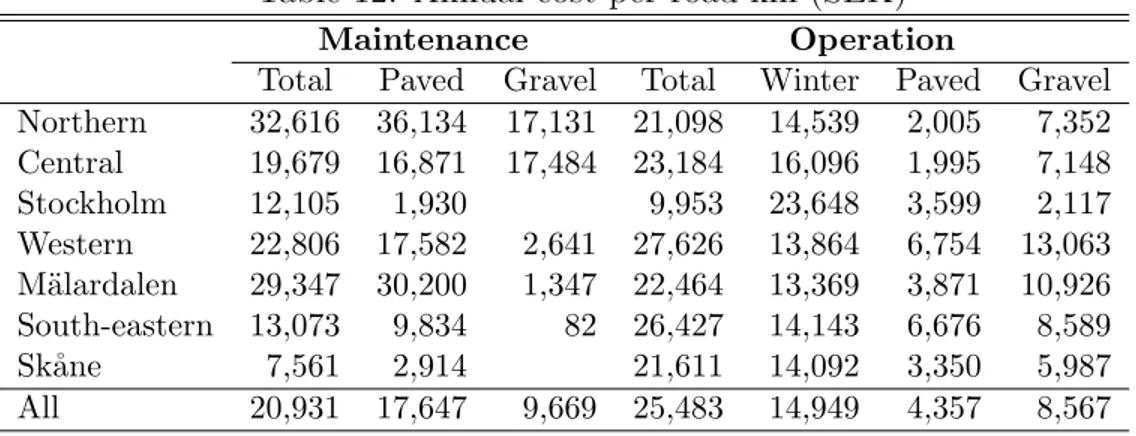
Table 12: Annual cost per road km (SEK)
Maintenance Operation
Total Paved Gravel Total Winter Paved Gravel
Northern 32,616 36,134 17,131 21,098 14,539 2,005 7,352 Central 19,679 16,871 17,484 23,184 16,096 1,995 7,148 Stockholm 12,105 1,930 9,953 23,648 3,599 2,117 Western 22,806 17,582 2,641 27,626 13,864 6,754 13,063 M¨alardalen 29,347 30,200 1,347 22,464 13,369 3,871 10,926 South-eastern 13,073 9,834 82 26,427 14,143 6,676 8,589 Sk˚ane 7,561 2,914 21,611 14,092 3,350 5,987 All 20,931 17,647 9,669 25,483 14,949 4,357 8,567