Performance analysis of different adapative algorithms based on acoustic echo cancellation

1

Performance Analysis of different Adaptive

Algorithms based on Acoustic Echo

Cancellation

Submitted by

Naga Swaroopa Adapa, Sravya Bollu

This thesis is presented as part of Degree in

Master of Science in Electrical Engineering with Emphasis on Signal Processing

School of Engineering Internet: www.bth.se/ing Blekinge Institute of Technology Phone: +46 455 385 000 371 79 Karlskrona Fax: +46 455 385 057 Sweden.

2

Contact Information:



Authors

1.Name: Sravya Bollu E- mail: srbb10@student.bth.se

2.Name: Naga Swaroopa Adapa E- mail: nasw11@student.bth.se



Supervisor 1

Name: Mr. Magnus Berggren

Dept: School Of Engineering (ING)

E-mail: magnus.berggen@bth.se Phone: +46 455 385 740



Supervisor 2

Name: Dr. Nedelko Grbic

Dept: School Of Engineering (ING) E-mail: nedelko.grbic@bth.se



Examiner

Name: Dr. Sven Johansson

Dept: School Of Engineering (ING) Email: sven.johansson@bth.se Phone no: +46455385710

3

ABSTRACT

In modern telecommunication systems like hands-free and teleconferencing systems, the problem arise during conversation is the creation of an acoustic echo. This problem degrades the quality of the information signal. All speech processing equipments like noise cancelling headphones and hearing aids should be able to filter different kinds of interfering signals and produce a clear sound to the listener. Currently, echo cancellation is a most interesting and challenging task in any communication system. Echo is the delayed and degraded version of original signal which travels back to its source after several reflections. Eliminating this effect without affecting the original quality of the speech is a challenge of research in present days. Echo cancellation in voice communication is a process of removing the echo to improve the clarity and quality of the voice signals. In our thesis we mainly focused on the acoustic echo cancellation in a closed room using adaptive filters. The Acoustic echo cancellation with adaptive filtering technique will more accurately enhance the speech quality in hands free communication systems. The main aim of using adaptive algorithms for echo cancellation is to achieve higher ERLE at higher rate of convergence with low complexity. The adaptive algorithms NLMS, APA and RLS are implemented using MATLAB. These algorithms are tested with the simulation of echo occurring environment by using constant room dimensions , microphone and source positions. The performance of the NLMS, APA and RLS are evaluated in terms ERLE and misalignment. The results show that RLS algorithm achieve good performance with more computational complexity comparing with the NLMS and APA algorithms. The NLMS algorithm has very low computational complexity comparing to RLS and APA algorithms. The results are taken for both input signal as speech signal and noise separately and plotted in the results section.

Keywords: Echo Cancellation, Adaptive algorithms, Noise Cancellation, Reverberation,

4

ACKNOWLEDGMENT

This thesis is dedicated to our parents who supported us with constant encouragement.

We would like to express our sincere gratitude and profound appreciation to our supervisors

Dr. Nedelko Grbic who gave us this opportunity to start the thesis work and Mr. Magnus Berggren who was a constant source of help and information, which helped us to successfully

complete our work. The timely advices and guidelines have assisted us to get through a lot of difficult situations.

We extend our thanks to our friends Sridhar Bitra and Harish Midathala for helping us throughout the thesis.

Above all we render immense gratitude to the ALMIGHTY GOD who bestowed self-confidence, ability and strength to complete this task

.

Finally I would like to thank all who support us and helped us in every aspect for completion of the thesis work.

5

CONTENTS

CHAPTER 1

INTRODUCTION

1.3 Hands free communication……….13

1.4 Problems in hands free communication………..14

1.4.1 Reverberation………..….…14 1.4.2 Background noise……….…14 1.4.3 Echo………...14 1.4.3.1 Hybrid echo………...15 1.4.3.2 Acoustic echo………...15 1.4 Objective of thesis………...16 1.5 Thesis organization……….16

CHAPTER 2 – ROOM IMPULSE RESPONSE

6

2.2.1 Direct sound………..……18

2.2.2 Early reverberation………..…..18

2.2.3 Late reverberation………...18

2.3 Room modelling………...19

2.4 Room image method………...19

2.5 Room parameters………...21

CHAPTER 3- ADAPTIVE FILTER ALGORITHMS

3.2 Adaptive filters………..…..22

3.2.1 General block diagram of the adaptive filter………...22

3.3 Applications of the adaptive filters………..……...23

3.3.1 System identification……….23

3.3.2 Noise cancellation in speech signals………...23

3.3.3 Signal prediction………...24

3.3.4 Interference cancellation………..….24

3.3.5 Acoustic echo cancellation………....25

3.4 Normalized Least Mean Square (NLMS) Algorithm……….25

3.4.1 Implementation of the NLMS algorithm………..26

3.4.2 Advantages and disadvantages………...26

3.4.3 Computational complexity………....26

3.5 Recursive Least Square (RLS) Algorithm………..27

3.5.1 Implementation of the RLS algorithm………..….…...27

3.5.2 Advantages and disadvantages………...………...27

3.5.3 Computational complexity……….…...27

7

3.6.1 Implementation of the affine projection algorithm………...…....28

3.6.2 Advantages and disadvantages………...…28

3.7 Various parameters that are to be considered when calculating the filter performance ………...29

CHAPTER 4 - ACOUSTIC ECHO CANCELLATION

4.2 Acoustic echo cancellation using adaptive filters………...31

CHAPTER 5 – IMPLEMENTATION

5.2 Room impulse response generation……….…….…..33

5.3 Echo cancellation using different adaptive algorithms………….…..………....34

5.4 Measurement of echo cancellation………..34

CHAPTER 6- RESULTS

6.2 Simulation results for echo cancellation using adaptive algorithms for pure speech as input for higher orders……….…42

6.3 Simulation results for echo cancellation using adaptive algorithm for noise as input for lower orders ………..…...44

6.4 Simulation results for echo cancellation using adaptive algorithm for noise as Input for higher orders ……….………..….49

CHAPTER 7 – CONCLUSION AND FUTURE SCOPE

8

7.2 Future work………...………..53

CHAPTER 8 - REFERENCES

9

LIST OF FIGURES

CHAPTER 1

Figure 1.1 Hybrid Echo ………..15

Figure 1.2 Acoustic Echo ………...…15

CHAPTER 2

Figure 2.2 A schematic diagram for representation of direct path, early reflections and late reflections……….18

Figure 2.3 Representation of first reflection path of image source……….19

Figure 2.4 Representation of the figure with two reflections………..20

Figure 2.5 Reverberated environment with reflected source images………..21

CHAPTER 3

Figure 3.2 System identification model………..23

Figure 3.3 Noise cancellation model………...23

Figure 3.4 Predicting future values of a periodic signal ………24

Figure 3.5 Interferences cancellation model ………..24

CHAPTER 4

10

CHAPTER 5

Figure 5.1 Room Impulse Response for higher orders….………..34 Figure 5.2 Room Impulse Response for higher orders ………..34 Figure 5.3 Implementation of adaptive algorithms for echo cancellation……..………35

CHAPTER 6

Figure 6.1 Input signal for NLMS, RLS and APA (speech signal)...……….37 Figure 6.2 Desired signal for NLMS, RLS and APA (speech signal)…………...………….38 Figure 6.3 Estimated error signal of NLMS algorithm (speech signal)………...…...38 Figure 6.4 Estimated error signal of RLS algorithm using filter length 400(speech signal)..39 Figure 6.5 Estimated error signal of APA algorithm using filter length 400(speech signal)..39

Figure 6.6 Comparison of NLMS, RLS and APA in terms of ERLE

For lower order (speech signal) ………...…...40 Figure 6.7 Misalignment of NLMS for different lower orders (speech signal)………….….40 Figure 6.8 Misalignment of RLS for different lower orders (speech signal)………..…....…41 Figure 6.9 Misalignment of APA for different lower orders (speech signal)………….…....41

Figure 6.10 Estimated error signal of NLMS algorithm using 4000 filter order (speech signal)……….…..42

Figure 6.11 Estimated error signal of RLS algorithm using 4000 order (speech signal)…..…42 Figure 6.12 Estimated error signal of APA algorithm using filter length 4000(speech signal)43 Figure 6.13 Misalignment of NLMS for higher orders (speech signal)………..…..…....43 Figure 6.14 Misalignment of RLS for higher orders (speech signal)…………...….………...44 Figure 6.15 Misalignment of APA for higher order (speech signal)……….…………...44 Figure 6.16 Desired signal of NLMS, RLS and APA algorithm (noise signal)……...……....45 Figure 6.17 Estimated error signal of NLMS using filter length 400 (noise signal)…….…...46 Figure 6.18 Estimated error signal of RLS using filter length 400 (noise signal)……....…...46 Figure 6.19 Estimated error signal of APA using filter length 400 (noise signal)…………..47

11

Figure 6.20 ERLE of NLMS, RLS and APA using filter length 400………..….47 Figure 6.21 Misalignment of NLMS for different lower orders(noise signal)….………48 Figure 6.22 Misalignment of RLS for different lower orders(noise signal)………..…...48 Figure 6.23 Misalignment of APA for different lower orders(noise signal)……….………....49 Figure 6.24 Estimated error of NLMS using filter length 4000 (noise signal)……….…49 Figure 6.25 Estimated error of APA using filter length 4000(noise signal)…….………...….50 Figure 6.26 ERLE of NLMS and APA for noise signal………...50 Figure 6.27 Misalignment of NLMS for different higher orders (noise signal)………...51 Figure 6.28 Misalignment of APA for different higher orders (noise signal)………..51

List of tables

Table 1: The details of clean speech ………..……. 32

LIST OF ABBREVIATIONS

AEC Acoustic Echo Cancellation

ANC Active Noise Control

PSTN Public Switched Telephone Network

NLMS Normalized Least Mean Square

RLS Recursive Least Square

APA Affine Projection Algorithm

RIR Room Impulse Response

12

ISM Image Source Method

FIR Finite Impulse Response

SNR Signal to Noise Ration

CR Convergence Rate

13

CHAPTER 1

1.1 Thesis organization:

This thesis report has been divided into 5 chapters. First chapter deals with the introduction and hands free speech communication problems.Second chapter deals with the room impulse response generation using room image method.The third deals with the implementation of the different adaptive algorithms such as, NLMS, RLS and APA and various parameters which calculates the performance of the adaptive algorithms.Fourth chapter shows the implementation of the acoustic echo cancellation with different adaptive algorithms.Fifth and six chapters include the implementation and results for the corresponding adaptive algorithms. The conclusion and proposed future work is dealt in the seventh chapter.

1.2 Introduction:

Speech enhancement is a globally rampant topic in research due to the use of speech enabled systems in a variety of real world telecommunication applications.The rapid growth of technology in recent decades has changed the whole dimension of communications.Today people are more interested in hands-free communication.This would allow more than one person to participate in a conversation at the same time such as a teleconference environment. Another advantage is that it would allow the person to have both hands free and to move freely in the room.However,the presence of a large acoustic coupling between the loudspeaker and microphone would produce a loud echo that would make conversation difficult.This is the main problem in hands free communication.When the speech signal is generated in the reverberated environment, the echo is created.This acoustic echo is actually the echo which is created by the reflection of sound waves by the walls of the room and other things that exist in the room such as chairs, tables etc.The solution to this problem is the elimination of the echo and provides echo free environment for speakers during conversation.This process of acoustic echo cancellation is truly useful in enhancing the audio quality of a hand free communication system.It prevents the listener fatigue and makes participants more comfortable.

1.3 Hands free communication:

Hands-free communication is used worldwide in modern telecommunication systems e.g. in hands-free telephones, videophones, audio and video conferences, mobile radio terminals or in speech recognition systems.It can be defined as the device which enables the user to use it without his hands.Hands-free communication involves a quite a number of technical problems such as room reverberation, acoustic echo and other ambient interferences [1].To improve the effectiveness of this hands-free communication, conventional methods like echo suppression and echo cancellation are used [2].

14

1.4 Problems in hands free communication

The major problem faced in most applications are background noise, reverberation and acoustic echo or acoustic feedback.Here is a brief description of each problem.

1.4.1 Reverberation:

Reverberation is the collection of reflected sounds from the surfaces in a closed environment, like a room.A reverberation is perceived when the reflected sound wave reaches the users ear in less than 0.1 second after the original sound wave.Reverberation occurs when the speech signal reaching the microphone undergoes multiple reflections, which affects the direct speech signal path.Reverberation time depends on the dimensions of the room, type of material used to construct the wall and the amount of sound absorbed by the wall.Even the number of people and items like chairs, tables also affect the reverberation time. Reverberation is a key factor in the design of theaters, concert halls and is controlled by lining the ceilings and walls with materials possessing specific sound-absorbing properties.The problem of reverberation can be decreased by reducing the distance between the microphone and the source of interest,thus the reflection from walls and ceilings becomes smaller compared to the direct sound.The removal of reverberation proves good in case of hearing aids.

1.4.2 Background noise :

Background noise refers to any sound element that causes disturbance or distraction.There are different types of background noises ranging from those that are almost undetectable to the ones that are extremely irritating.These days background noise has become much prevalent and is caused by engines, fan noise in computers, traffic, industries and in public places.These sources of noise tend to degrade the performance of the receiver. Disturbances occur from every direction, they are assumed to be the surrounding noise. Background noise contains higher level of low frequency when compared to speech signal, hence an active noise control can come to aid, since convention methods of suppressing noise do not work well at low frequencies [3].

1.4.3 Echo:

Echo is the delayed and degraded version of original signal which travels back to its source after several reflections.Nature of echo signal can be either acoustic or electrical, and in order to reduce its undesired effect we employ echo cancellers.

Echoes in telecommunication are categorized as two types [4], namely 1. Hybrid echo

15

Fig: 1.1 Hybrid Echo [16] 1.4.3.1 Hybrid echo

This type of echo is mainly seen in public switched telephone network (PSTN).These hybrid echoes arise when signals reflect at the point of impedance mismatch in a circuit.This is generally found where the telephone local loops are 2-wire circuits and transmission line is a 4- wire circuit.Each hybrid produces echoes in both directions, though the far end echo is usually a greater problem for voice band.

1.4.3.2 Acoustic echo:

Fig: 1.2 Acoustic Echo [16]

Acoustic echo occurs when an audio signal is reverberated in a real environment, resulting in original signal plus the attenuated signal.The signal interference caused by acoustic echo is

16

distracting to both the users and causes a reduction in quality of communication.Popular methods for echo cancellation in hands-free telephony are based on adaptive filtering techniques.This type of echo results from a feedback setup between the speaker and the microphone in mobile phones, hands-free phones, teleconferences or hearing aids systems. Acoustic echo is reflected from a multitude of different surfaces like wells, ceilings and floors and travel through different paths.These echoes can also result from a combination of direct acoustic coupling from various surfaces and picked up by the microphone.The worst case of an acoustic echo is when acoustic feedback results in howling if a significant propagation of sound energy is transmitted by loudspeaker is received back at the microphone and circulated in feedback loop.Howling occurs when both parties have hands-free systems with open speakers and microphones.It mainly occurs in an auditorium.

1.5 Objective of thesis:

The main objective of our thesis is to study and simulate the acoustic echo cancellation using different adaptive algorithms.We implemented different adaptive algorithms such as, Normalized Least Mean Square(NLMS) algorithm[9],Recursive Least Square (RLS) algorithm[9] and Affine Projection Algorithm(APA)[9].We also implemented room impulse response function (RIR) using mirror image method.A predefined input signal with 16 KHz is filtered with the room impulse response generator output, to generate an acoustic echo signal.Echo Return Loss Enhancement was used to evaluate the performance of echo loss provided by the adaptive filters.If the echo return loss enhancement increases the amount of echo cancellation also increases.Higher echo return loss enhancement results in better performance.

17

CHAPTER 2

RIR - ROOM IMPULSE RESPONSE

2.1 Basic concept of reverberation:

In large rooms like an auditorium there will be a considerable effect of reflections on the received speech.If the source of sound is suddenly turned off, there will be some observed residual sound.This is due to so called effect of ‘reverberation’.It is undesirable effect for speech and desirable effect in music [5].Reverberation time is a pivotal parameter to characterize the room reverberation.It is defined as the time required for reflections of a direct sound to decay 60 dB below the level of the direct sound.The factors that contribute to reverberation time are size of the room, number of items in the room (people, tables, chairs) and the constructing materials of room (concrete, ceramics, hardware).The room surfaces determine the absorption coefficients and the amount of energy lost during reflection.For speech to be intelligible, reverberation time must be less than two seconds.In a situation when an individual needs to speak with the audience reverberation must be eliminated or minimized.

2.2 Reverberation:

Fig: 2.1 Illustration of direct sound, early reverberation and late reverberation.

Reverberation is the process of multi-path propagation of an acoustic signal from its source to the microphone. It is based on the concept of reflections.The desired sound source produces

18

wave fronts, which propagate outward from the source.These wavefronts reflect off the walls of the room and superimpose at the microphone.Due to differences in the lengths of the propagation paths to the microphone and in the amount of sound energy absorbed by the walls, each wave front arrives at the microphone with a different amplitude and phase.The term reverberation designates the presence of delayed and attenuated copies of the source signal in the received signal.In the above figure 2.1 we can clear see the reflections of the sound.

Room reverberation is a result of a number of reflections of sound, they can be divided into three sound components:

2.2.1 Direct sound: The first sound that is reached through the free medium i.e. air without

any reflection is called direct sound.If the source is not in the line of sight of the observer then there is no direct sound.

2.2.2 Early reverberation: The sounds which have undergone reflections to one or more

surfaces such as walls, floors, furniture are received after a short time.The reflected sounds are separated in both time and direction from the direct sound.These reflected sounds combine to form a sound component called early reverberation.Early reflections are the impulses that arrive within 50ms after the direct signal [4].

2.2.3 Late reverberation: The sound reflections which arrive with larger delays after the

arrival of the direct sound.These sound reflections are perceived as separate echoes and reduces speech intelligibility.Late reflections, in turn, which arrive at time intervals greater than 50ms.Fig 2.2 represents diagram for representation of early reflections and late reflections [14].

19

2.3 Room modeling: In our thesis, we used image method to calculate the impulse response

of the room. The working of the room model can be explained as follows:

 Visualizing the individual echoes that produce disturbance.

 Finding the unit impulse response of each echo with proper time delay.

 Calculating the magnitude of individual echo’s unit impulse response.

The time and magnitude of each echo is being calculated as if it is the echo is being heard from a particular position in the room.All this information put together into a one dimensional function of time which will be the room impulse response.

2.4 Room image method: The image source method has become a ubiquitous tool in many

fields of acoustics and signal processing.Image Source Method (ISM) represents a principle of considerable importance for engineering and acoustics research community.An important practical application of ISM concept is related to performance assessment of various signal processing algorithms operating in reverberant environment.The image model is used to simulate the reverberation in a room for a given source.The microphone location is discussed in this section.Using the image method Allen and Berkley [6] developed an efficient method to compute a Finite Impulse Response (FIR) that models the acoustic channel between a source and a receiver in rectangular rooms.

Fig: 2.3 Representation of the first reflection path of the image source.

In the above fig 2.3 a sound source S located near a rigid reflecting wall. At destination D two signals arrive, one from the direct path and second one from the reflection.The path length of the direct path can be directly calculated from the known locations of the source and

20

Fig: 2.4 representation of the figure with two reflections

equal to the distance of the source from the wall. Because of symmetry, the triangle SR is isosceles and therefore the path length SR+RD is the same as . Hence to compute the path length of the reflected path, we can construct an image of the source and compute the distance between destination and image.Also, the fact that we are computing the distance using one image means that there was one reflection in the path. In the fig 2.4 it shows a path involving two reflections.The length of this path can be obtained from the length of D.These figures can also be extended to three dimensions to take into the account reflections from the ceiling and the floor.The strength of the reflection can be obtained from the path length and the number of reflections involved in the path.The number of reflections involved in the path is

Fig 2.5 reverberated environment with reflected source images

equal to the level of images that was used to compute the path.The above figure 2.5 shows a sound source (green circle) located in a room at 3D position. Red plus(+) symbol is considered to be origin point [23] or midpoint of the room and its coordinates are assumed to be (0,0,0). Every position is measured with reference to the origin of the room. is distance between the microphone and origin. is the distance between source and the origin. is the reflecting wall distance from the origin.The source 1 and source 2 are the first reflected image sources generated from reverberating image model [7].The whole early and late reverberation source image positions ( , ) are calculated as follows:

+ [i+ ]

+ [j+ ]

-21

= =

Where, c is the velocity of sound in meters. is the value estimated for multiple reflections of reverberation.For every reflection there should be some loss of energy which is estimates using reflection coefficient (α) alpha.

2.5 Room parameters:

There are various factors that affect the room impulse response. The major factors are:

 Position of the source

 Reflection coefficient

 Absorption coefficient

22

CHAPTER 3

ADAPTIVE FILTER ALGORITHMS 3.1 Introduction to adaptive filters:

Basically, filtering is a signal processing technique whose objective is to process a signal in order to manipulate the information contained in the signal.In other words, a filter is a device that maps its input signal into another output signal by extracting only the desired information contained in the input signal.An adaptive filter is necessary when either the fixed specifications are unknown or time-invariant filter cannot satisfy the specification. Strictly speaking an adaptive filter is a nonlinear filter since its characteristics are dependent on the input signal and consequently the homogeneity and additively conditions are not satisfied. Additionally, adaptive filters are time varying since their parameters are continually changing in order to meet a performance requirement.

3.2 Adaptive Filters

3.2.1 General block diagram of the adaptive filters:

Here w represents the coefficients of the FIR filter tap weight vector, x(n) is the input vector sample, is a delay of one sample, y(n) is the adaptive filter output, d(n) is the desired echoed signal and e(n) is the estimation of the error signal at time n.

The aim of an adaptive filter is to calculate the difference between

the desired signal and the adaptive filter output, e(n).The error signal is fed back into the adaptive filter and its coefficients are changed algorithmically in order to minimize a function of this difference, which is known as the cost function [8].

Fig: 3.1 Block diagram of adaptive filter

In the case of acoustic echo cancellation, the optimal output of the adaptive filter is equal in value to the unwanted echoed signal. When the adaptive filter output is equal to desired signal the error signal goes to zero.In the situation the echoed signal would be completely cancelled and the far user would not hear any of their original speech returned to them.

23

3.3 Applications of adaptive filters: 3.3.1 System identification:

Fig: 3.2 System identification model

System identification refers to the ability of an adaptive system to find the FIR filter that best reproduces the response of another system.This works perfectly when the system to be identified has got a frequency response that matches with the certain FIR filter. It will never be able to give zero output but it may reduce it by converging to an optimum weights vector. The frequency response of the FIR filter will not be exactly equal to that of the unknown system but it will certainly be the best approximation to it . The above figure 3.2 [9]shows a typical system identification configuration, where is an ideal coefficient vector of an unknown system, whose output is represented by and n(k) is the observed noise.

3.3.2 Noise cancellation in speech signals

24

The above figure 3.3 shows adaptive noise cancellation model[9].Adaptive filtering technique is widely used in cases where a speech signal is submerged in a very noisy environment. The adaptive noise canceller for speech signal needs two inputs. The main input contains the speech which is corrupted by noise. The other input contains noise related in some way to the main input signal which is the reference signal. The system filters the noise reference signal to make it more similar to that of the main input signal and that filtered version is subtracted from the main input. Ideally it removes the noise and leaves exact speech. In practical systems noise is not completely removed but its level is reduced considerably.

3.3.3 Signal prediction:

Fig: 3.4 Predicting future values of a periodic signal

Predicting signals is one of the impossible task, without some limiting assumptions. Here the function of the adaptive filter is to provide best prediction of the present value of a random signal. Accepting some assumptions, the adaptive filter must predict the future values of the desired signal based on past values. When s(k) is periodic and the filter is too long to remember the previous values, this structure with the delay in the input signal can perform the prediction. The adaptive filter input signal x(k) is a delayed version of the reference signal d(k). Therefore when the adaptive filter output y(k) approximates the reference signal, the adaptive filter operates as a prediction system.The above figure 3.4 represents the predicting future values of a periodic signal[9].

3.3.4 Interference cancellation:

In this application, adaptive filter is used to cancel unknown interference in the primary signal. The primary signal serves as the desired response for the adaptive filter. A reference signal is employed as the input to the adaptive filter. A signal of interest s(k) is corrupted by a noise component n(k). The noisy signal s(k) + n(k), is then employed as the reference signal for the adaptive fiter, whose input should be another version, (k) which is correlated to n(k).The filter adjusts the filter coefficients in such a manner that the filter output y(k) approximates x(k) forcing the error signal e(k) to resemble the signal s(k).The below figure3.5 represents the interference cancellation model[9].

25

Fig: 3.5 Interference cancellation model

3.3.5 Acoustic echo cancellation:

An acoustic echo is the common occurrence in today’s telecommunication system. It occurs when the input and output operate in full duplex mode; an example of this is a hands free telephone.In this situation the received signal has outlet through the loudspeaker, the audio signal is reverberated through the physical environment and picked up by the microphone.This effect causes time delay and attenuates the original speech signal, hence reducing the speech quality [9].In the case of acoustic echo in telecommunications, the optimal output is an echoed signal that accurately emulates the unwanted echo signal. This is then used to reduce the echo in the return signal.The better the adaptive filter reduces this echo, the more successful the cancellation will be.

3.4 Normalized least mean square algorithm:

The LMS is based on steepest descent algorithm. LMS algorithm is used widely for different applications such as channel equalization and echo cancellation.This algorithm is used due to its computational simplicity. Computational complexity for LMS is 2N+1 multiplications and additions. The equation below is LMS algorithm for updating the tap weights of the adaptive filter for each iteration [10].

w(n+1)=w(n)+µe(n)x(n) (1) Where x(n) = is the input vector of time delayed input

values and

w(n) = is the weight vector at the time n

One of the primary disadvantages of the LMS algorithm is that it has a fixed step size for each iteration.Determining the upper bound step size is a problem for the variable step size algorithm, if the input signal to the adaptive filter is non-stationary.A convenient way to incorporate this step size into the LMS adaptive filter is to use a time varying step size. NLMS is an extension of the LMS algorithm which bypasses the issue by selecting a different step size value µ(n) ,for each iteration of the algorithm.Step size is inversely proportional to the inverse of the total expected energy of the instantaneous values of coefficients of the input vector x(n).

26

3.4.1 Implementation of the NLMS algorithm:

 The output of the adaptive filter is calculated as

y(n) = = (n) x(n) (2)

 An error signal is calculated as the difference between the desired signal and the filter output

e(n) = d(n) – y(n) (3)

 The step size value for the input vector is calculated as

µ(n) = (4)

 The filter tap weights are updated for the next iteration

w(n+1) = w(n)+µ(n)e(n)x(n) (5)

3.4.2 Advantages and disadvantages:

 NLMS algorithm has low computational complexity, with good convergence speed which makes this algorithm good for echo cancellation.

 It has minimum steady state error.

 The noise amplification becomes smaller in size due to the presence of normalized step size.

3.4.3 Computational complexity:

 NLMS requires more number of computations for evaluation when compared to LMS algorithm due to the presence of the reference signal power.

 NLMS algorithm requires 3N+1 multiplications which is N times more than the LMS algorithm. Where N is the length of the coefficient vector.

3.5 Recursive least square (RLS):

In this algorithm w(n) updates continuously with each set of new data without solving matrix inversion.The least square algorithms require all the past samples of the input signal as well as the desired output at every iteration.RLS filter is a simple adaptive and time update version of Weiner filter.For non-stationary signals, this filter tracks the time variations but in case of stationary signals, the convergence behavior of this filter is same as weiner filter.This filter has fast convergence rate and it is widely used in the application such as echo cancellation, channel equalization, speech enhancement and radar where the filter should do fast changes in signal.

27

3.5.1 Implementation of the RLS algorithm: First two factors of the RLS implementation

should be noted: the first is that although the matrix inversion is essential for the derivation of RLS algorithm, no matrix inversion calculations are required for the implementation, hence reducing the computational complexity of the algorithm.Secondly, unlike the LMS based algorithms, current variables are updated within the iteration using values from the previous iteration [9].The computational data for RLS algorithm is as follows

λ= Exponential weighting factor

δ= value used to initialize inverse of Autocorrelation at n=0 i.e., P(0)= _I

I= Identity matrix

P(n) = inverse of the Autocorrelation matrix (n), where

(n)= (5) g(n)= gain vector = (6) z(n) = P(n-1)x(n) (7) g(n) = z(n) (8)

The estimation error is calculated using equation

e(n) = d(n)- (n)x(n) (9) The adaptive filter coefficients and in turn the coefficients of auto correlation matrix are calculated as

w(n) = w(n-1) + e(n)g(n) (10) P(n) = [P(n-1)-g(n) (11)

3.5.2 Advantages and disadvantages:

 It converges faster than LMS in stationary environment but in non-stationary LMS is better than RLS.

 Sensitive to computer round off error which leads to instability.

 Greater computational complexity.

 Numerically robust RLS is of two types:Square root RLS and inverse QR RLS algorithm.

28

3.5.3 Computational complexity:

 Each iteration of the RLS algorithm requires 4N^2 multiplication operations and 3N^2 additions.This makes implementation costly.

3.6 Affine projection algorithm:

The affine projection algorithm (APA) is a generalization of the well-known normalized least mean square (NLMS) adaptive filtering algorithm.The affine projection algorithm is an ’intermediate’ algorithm in between two well-known algorithms NLMS and RLS. It has both performance and complexity between these two adaptive algorithms.Under this interpretation, each tap weight vector in the update of NLMS is viewed as a one dimensional affine projection.In APA the projections are made in multiple dimensions.In APA, a high projection order leads to a fast convergence rate but a large estimation error.Meanwhile, a low projection order gives rise to a slow convergence rate but a small estimation error.Affine projection algorithm includes LMS like complexity.Affine projection algorithm is that it causes no delay in the input or output signals.These features make APA an excellent candidate for adaptive filter in the acoustic echo cancellation problem.It is well known that fast affine projection algorithms can produce a good trade-off between convergence speed and computational complexity [12].

3.6.1 Implementation of affine projection algorithm:

Let us assume we keep L+1 input signal vectors in a matrix as follows:

X(n)= =[ (12) d(n)= (13) e(n)= (14)

where L is the projection order of APA

e(n)= d(n)- (n)w(n) (15)

The objective of the affine projection algorithm is to minimize

29

Subject to:

d(n)- (n)w(n)=0 (17)

w(n)= w(n-1)+µX(n) _{e(n) (18)} where γ is small constant, µ is taken in the range of 0< µ ≤ 2

This equation is a generalization of the NLMS and the RLS algorithms.If N=1 the algorithm becomes NLMS algorithm where n is the number of samples and if N=n it is equivalent to the RLS algorithm.One of the way in which LMS and APA algorithms can be compared is that, LMS algorithm calculates the error, as the performance of the last updated echo estimate vector based on current input vector,whereas APA algorithm calculates the error as the performance of the last updated echo estimate vector based on the previous N input vectors [12].

3.6.2 Advantages and disadvantages:

 APA has faster tracking capabilities than NLMS.

 APA has a better performance in steady state mean square error (MSE) or transient response compared with other algorithms.

 APA has better performance than NLMS and better complexity than RLS.

3.7 Various parameters that are to be considered when calculating the filter performance are:

 Convergence rate (CR):Convergence rate is a performance specification of acoustic

echo cancellers.The convergence rate should be fast to estimate the desired filter.The convergence rate is defined as the number of iterations required for the algorithm to converge to its steady state mean square error [13].

 Estimated error:Mean square estimation is the average of the squares of the error.

The mean square estimation is given as

= (15)

 Echo return loss:This is expressed as the difference between the echo signal level and

speech signal level generally expressed in dB.

 Echo return loss enhancement:It is the ratio of the instantaneous power of the echo

30

 Complexity:The computational complexity is the measure of the number of arithmetic

calculations like multiplications, additions and subtractions for different adaptive algorithms.

 Signal to noise ratio (SNR):The Signal-to-Noise Ratio is used to measure the amount of desired signal level with the noise level.The ideal method for calculating the SNR is the amount of speech energy over the noise energy after the enhancement method.The input SNR and output SNR are calculated as below:

= /n (16)

=10

/n (17)

Where and are the filtered outputs of the Wiener beamformer i.e.pure speech signal s(n) and pure noise signal d(n) separately and also ‘n’ is the length of the speech and

noise signals. [14]

31

CHAPTER 4

ACOUSTIC ECHO CANCELLATION

4.1 Introduction:

Echo cancellation is a widely used digital signal processing technique.Speech by the far end speaker is captured by the near end microphone and sent back in the form of echo.Acoustic echo is defined as a type of noise which occurs due to the reflections of speech signal by the walls, ceiling or objects of a room.Acoustic echo causes great discomfort to the users since their own speech is heard during conversation [15].The main aim of the hands-free communication is to cancel the acoustic echo in order to provide echo free environment.An acoustic echo canceller can overcome the echo that interferes with teleconferencing and hands free telecommunications.The present study deals with canceling these echo signals for improving the communication quality by using various adaptive filtering algorithms which we discussed in the chapter 3 and comparing the performance of all these algorithms.

.

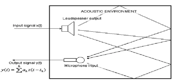
Fig: 4.1 Origins of acoustic echo

When an input signal is received by the system, it is sent to the loudspeaker into the acoustic environment.This signal is reverberated within the environment and returns back to the system via the microphone.These reverberated signals contain time delayed images of the original speech.This scenario is clearly shown in figure 4.1. Here is the attenuation, is the time delay.This occurrence of the acoustic echo causes signal interference and reduces the quality of communication.

32

4.2 Acoustic echo cancellation using adaptive algorithms:

Acoustic echo control is widely used application area. Designing adaptive filters is an

important task, which we obtained in the chapter 3. Adaptive filters are dynamic filters which iteratively alter their characteristics in order to achieve an optimal desired output. An adaptive filter algorithmically alters its parameters in order to minimize a function of the difference between the desired output d(n) and its actual output y(n).This function is known as the cost function of the adaptive algorithm [9].

The aim is to cancel the desired input signal d(n) by making sure the error signal e(n) is kept to the best minimum value possible.From fig 4.2 it is noted that the past values of the estimation error signal e(n) is fed back to the adaptive filter.The purpose of the feedback is to effectively adjust the structure of the adaptive system, thus altering its response characteristics to the optimum possible value.Simply, the adaptive filter is self-adjusting hence the name ’adaptive’.

Below fig 4.2 shows an acoustic echo cancelling setup.Let x(n) be the input signal(from the far end speaker) travelling to the near end speaker through the loud speaker and d(n) is the signal picked up by the microphone which in this case is the far end echo. h(n) represents the impulse response of the acoustic environment.w(n) represents the adaptive filter used to cancel the echo signal.The adaptive filter equate its output y(n) to the desired output d(n) ( the signal reverberated within the acoustic environment). At each iteration the error signal e(n) = d(n)-y(n) is fed back into the filter, where the filter characteristics are altered accordingly. In the case of acoustic echo cancellation, the optimal output of the adaptive filter is equal in value to the unwanted echoed signal.When the adaptive filter output is equal to desired signal the error signal goes to zero. In the situation the echoed signal is completely cancelled and the far user would hear a clear speech.

33

CHAPTER 5

IMPLEMENTATION

5.1 Introduction:

The main purpose of this thesis is the elimination of acoustic echo and disturbances which occur in hands free speech communication.Echo cancellation using adaptive algorithms NLMS, RLS and APA are implemented using Matlab.We have discussed in detail the implementation of the adaptive algorithms in the chapter 3. Among the available schemes of room modeling, the image method was chosen for calculation of room impulse response. A predefined speech input signal SPEECH_ALL of sampling frequency 16000Hz is convoluted to the RIR, to generate an acoustic echo signal which serves as the input to the echo canceller and results are taken and plotted in results section for each adaptive algorithm. The details of the clean speech signal SPEECH_ALL is shown in the below table 1.After that white Gaussian noise is taken in the input signal.Results taken for the three algorithms and plotted in the results section.

Table 1:

File name Duration in sec Type of

voice

Sentences

3 Female “It is easy to tell the depth of

the well”.

Speech _all.wav 2 Male Kick the ball straight and

follow through”.

3 Female “Glue the sheet to the dark

blue back ground”.

3 Male “A part of tea helps t3o pass

the evening”.

Table 1: The details of clean speech used for the evaluation.

5.2 Room impulse response generation:

We considered the room dimensions as [6,4,6] meters with microphone position as [5,2,1] and speaker position as [2,3,1] which are separated by some distance. The order of this RIR function is taken from [1000, 2000, 3000 and 4000] samples the reflection

coefficient is taken as 0.7. For the choosen reflection coefficient and the room dimensions , the reverberation time is 0.14 sec. The possible values of the reflection coefficient must be in between the interval [-1,1]. Generally the value of the reflection coefficient is positive. The

34

parameters which play key role in modeling RIR are reflection coefficient of the wall, size of the room, position of the room and position of the microphone in the room assuming that room does not contain any obstacles.With desired room dimensions and parameters, RIR is generated using Image method. The corresponding output for the RIR is shown in figure 5.1. For both NLMS and APA algorithms we considered this RIR function.

Fig: 5.1 Room impulse response for higher order

We also considered lower order for the evaluating the performance of the adaptive algorithms this is because RLS algorithm for higher order is taking more time to converge.It takes 2 hours minimum for the algorithm to converge.For this reason we take the order of this RIR function from [100, 200,300,400] and also reduced the size of the room by a factor of 10.The corresponding output for the RIR is shown in the figure 5.2.

35

Fig 5.2 Room impulse response output for lower order

5.3 Echo cancellation using different adaptive algorithms:

Fig: 5.3 Implementation of adaptive algorithms for echo cancellation.

In our thesis NLMS and APA adaptive algorithm is implemented for both lower and higher orders i.e. [1000, 2000, 3000, and 4000] are considered for higher order and [100,200,300,400] are considered as lower order,RLS algorithm is considered only for the lower orders in our thesis because it is taking more time to converge compared with the other two algorithms.The step size µ is set to 0.9 for NLMS algorithm, for RLS step size δ is taken as 0.001 and λ is set to 0.99, step size µ for APA is considered as 0.1.The above fig: 5.3 shows the implementation of the different adaptive algorithms for echo cancellation.The input to the echo canceller x(n) is the pure speech signal, d(n) is the desired signal which contains echo signal, e(n) is the error signal. The error signal should be as minimum as possible to get the best echo cancellation.For comparison with the speech signals we considered white Gaussian noise in the input signal.The amount echo cancellation is calculated in terms of the echo return loss enhancement and misalignment.So in the results section we plotted ERLE and misalignment graphs for both pure speech signal and noisy input signal.

5.4 Measurement of the echo cancellation: Echo return loss enhancement (ERLE):

Echo return loss enhancement is the ratio of input desired signal power and the power of a residual error signal immediately after echo cancellation.It is measured in dB. ERLE depends on the size of the adaptive filter and the algorithm design.The higher the value of ERLE represents the better echo cancellation.It also measures the amount of loss introduced by the adaptive filter.ERLE is a measure of the echo suppression achieved and is

36

given by [16].The ERLE measurement helps to calculate echo loss done by the adaptive algorithm.In our simulations we noticed that ERLE increases with the increase in the order of the filter.

ERLE = 10 ( )

Where is the desired signal power and is the power of a residual error signal after echo cancellation.

Misalignment

:

In our thesis we also evaluated the performance of the echo canceller in terms of the misalignment as defined by

ϵ=

where || . || denotes the norm of a vector and h = [h(0),…..h(L-1)]. It measures the mis-match between the true and the estimated impulse response of the receiving room. Receiving room is where the acoustic coupling between the loud speaker and the microphone happens and thus echo generates [18].

37

CHAPTER 6

RESULTS

First we take the results for lower order for three algorithms and then we took results for higher order for NLMS and APA algorithms. For higher orders RLS algorithm takes more time to converge. The RLS algorithm required 4N^2 multiplications per iteration , as for echo cancellation the order is usually in thousands in real time ,the number of multiplications required is very large making RLS algorithm too costly to implement. So we only used RLS for the lower order.The results show that RLS algorithm has good performance with higher rate of convergence speed comparing with the NLMS and APA algorithms, but the computational complexity is very high which is impractical in real time applications. The performance of APA algorithm in echo cancellation is higher than NLMS algorithm with less computational complexity than RLS.Secondly we evaluated the performance of the three algorithms in terms of misalignment.Results show the RLS algorithm has good echo cancellation when compared with other algorithms in terms of misalignment.For comparison with the speech signal performance we have taken results for noise signal as input.The results show that the noise input signal take much less time to converge.

6.1 Simulation results for echo cancellation using adaptive algorithm for pure speech as input for lower orders.

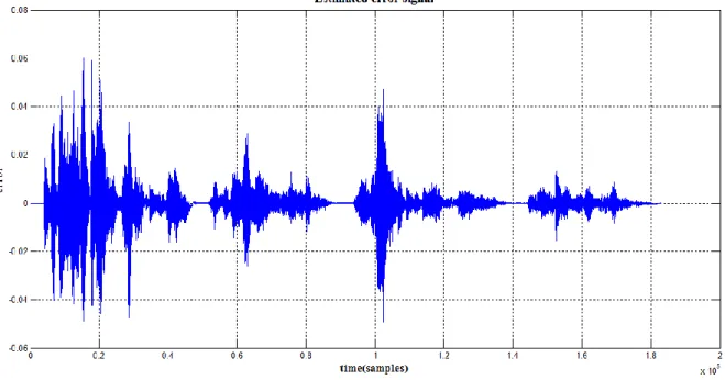
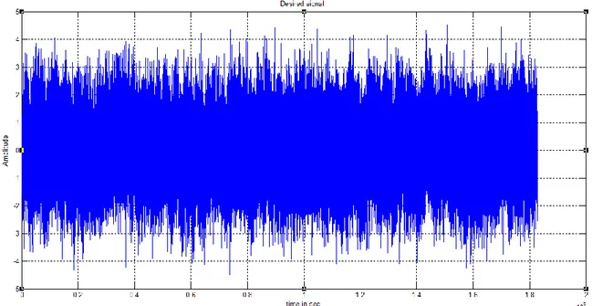
38 Fig: 6.2 desired signal for NLMS, RLS and APA algorithms (speech signal) The figure 6.3 shows the error signal estimated with the adaptive filtering with NLMS

algorithm of order 400.

Fig: 6.3 estimated error signal of NLMS algorithm using filter length 400(speech signal)

The figure 6.4 shows the error signal estimated with the adaptive filtering with RLS algorithm of order 400.

39

Fig: 6.4 estimated error signal of RLS algorithm(speech signal) using filter length 400.

The figure 6.5 shows the error signal estimated with the adaptive filtering with APA algorithm of order 400.

40

Figure 6.6 shows the comparison of NLMS, RLS and APA in terms of ERLE with order 400. It shows the amount of echo cancellation after adaptive filtering with NLMS, RLS and APA algorithms.

Fig: 6.6 comparison of NLMS, RLS and APA in terms of ERLE for lower order (speech signal)

Figure 6.7 shows the misalignment of NLMS algorithm for different orders.

41 Figure 6.8 shows the misalignment of RLS algorithm for different orders.

Fig: 6.8 misalignment of RLS for different lower orders (speech signal)

Figure 6.9 shows the misalignment of APA algorithm for different orders.

42

6.2 Simulation results for echo cancellation using adaptive algorithm for pure speech as input for higher orders.

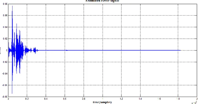
Figure 6.10 shows the estimated error signal of NLMS algorithm with the order 4000.

Fig: 6.10 estimated error signal of NLMS using filter length 4000(speech signal)

Figure 6.11 shows the estimated error signal of APA algorithm with the order 4000.

43 Figure 6.12 shows that the ERLE for NLMS and APA algorithm for order 4000.

Fig: 6.13 misalignment of NLMS for higher orders (speech signal)

44 Fig: 6.14 misalignment of APA algorithm for higher orders (speech signal)

6.3 Simulation results for echo cancellation using adaptive algorithm for noise as input for lower orders.

45

Fig: 6.16 desired signal of NLMS, RLS and APA (noise signal)

The figure 6.17 shows the error signal estimated with the adaptive filtering with NLMS algorithm of order 400.

46

The figure 6.18 shows the error signal estimated with the adaptive filtering with RLS algorithm of order 400.

Fig: 6.18 estimated error signal of RLS using filter length 400 (noise signal)

The figure 6.19 shows the error signal estimated with the adaptive filtering with RLS algorithm of order 400.

47

Figure 6.20 shows the comparison of NLMS, RLS and APA in terms of ERLE for noise as input signal with order 400. It shows the amount of echo cancellation after adaptive filtering with NLMS, RLS and APA algorithms.

Fig: 6.20 ERLE of NLMS, RLS and APA using filter length 400 (noise signal)

48 Fig: 6.22 misalignment of RLS for different lower orders (noise signal)

49

6.4 Simulation results for echo cancellation using adaptive algorithm for noise as input for higher orders.

The figure 6.24 shows the error signal estimated with the adaptive filtering with NLMS algorithm of order 4000.

Fig: 6.24 estimated error of NLMS using filter length 4000 (noise signal)

The figure 6.25 shows the error signal estimated with the adaptive filtering with APA algorithm of order 4000.

50 Figure 6.26 shows the ERLE of NLMS and APA algorithm for noise input signal with order 4000

.

51 Figure 6.28 shows the misalignment of APA for noise signal as input with different orders.

Fig: 6.28 misalignment of APA for different higher orders (noise signal)

52

CHAPTER 7

Conclusion:

This research was initiated with the aim of evaluating the performance of three different adaptive algorithms:NLMS, RLS and APA algorithms based on acoustic echo cancellation.A room is created using room image method.The input to the echo canceller is created by the convoluting the speech signal with the room impulse response (RIR) output, which generates acoustic echo signal.So echo canceller is implemented using the three algorithms and the performance of different adaptive algorithms are compared.The performance of the adaptive algorithms is calculated in terms of ERLE and misalignment. After that the input to the echo canceller is taken as white Gaussian noise and the results are compared for the three adaptive algorithms.

The difference between ERLE and misalignment measurement is that when the filter length increases the minimum error value decreases and the ERLE increases. It is measure of echo loss provided by the adaptive filters.In misalignment measurement when the filter length increases the degree of misalignment increases. Misalignment is used to tell how faster the adaptive algorithm converge.The error decreases but does not come to zero, practically it is impossible when the adaptive filter is unstable. We can try reducing the step size and stabilize the adaptive filter.

Results are presented individually for lower orders and higher orders for both speech and noise signals.Difference between the noise and speech signal is that speech signal take more time to converge when compared to noise signal.When the final results were observed, it was clearly observed that RLS algorithm exhibits higher ERLE value for lower orders. For higher orders we only considered APA and NLMS algorithm. Since RLS takes more time to converge we excluded RLS. For this we got higher ERLE for APA algorithm compared with NLMS.The NLMS algorithm has less computational complexity and very easy to implement in real time, but it gave the poor performance compared with the other two adaptive algorithms. The echo cancellation performance of the APA is in between NLMS and RLS algorithms.Another parameter that was used for the performance analysis of the adaptive algorithms is misalignment. For both lower and higher orders the results for misalignment is taken separately for NLMS, RLS and APA algorithms.We observed that when the order increases degree of misalignment decreases for each algorithm.

Future work:

Future work can be extended by implementing the experimental setup for the double talk situations.Double talk is an important characteristic of a good acoustic echo canceller. It is a condition where both the, far-end user and near-end user speak simultaneously.Comparing the performance of double talk detector with the other adaptive algorithms is also equally im-portant.

53

The work in thesis is regarded as work in offline mode so implementing the system for real time can be done in future work.There is a lot, which can be done in future for im-provement on the methods for acoustic echo cancellation.The field of digital signal processing and in particular adaptive filtering is vast and further research and development in this area can result in bigger improvements.

References

[1] I. Papp, Z. Saric and N. Teslic, "Hands-free voice communication with TV," Consumer

Electronics, IEEE Transactions on , vol.57, no.2, pp.606-614, May 2011.

[2] J. Benesty, D. Morgan and M. Sondhi, "A hybrid mono/stereo acoustic echo canceler," Speech and Audio Processing, IEEE Transactions on , vol.6, no.5, pp.468-475, Sep 1998. [3] J.-S. Park, B.-K. Kim, J.-G. Chung and K. Parhi, "High-speed tunable fractional-delay

allpass filter structure," Circuits and Systems, 2003. ISCAS '03. Proceedings of the 2003 International Symposium on , vol.4, no., pp. IV-165- IV-168 vol.4, 2, 25-28 , May 2003. [4] M. Harish, "Speech Enhancement in Hands-free Communication with emphasis on

Optical SNIR Beamformer," M.S. Thesis, Dept. of Signal Processing., Blekinge Tekniska Hogskola, BTH, Sweden, 2012.

[5] N. Shabtai, Y. Zigel and B. Rafaely, "The effect of room parameters on speaker verification using reverberant speech," Electrical and Electronics Engineers in Israel, 2008. IEEEI 2008. IEEE 25th Convention of , pp.231-235, 3-5, Dec. 2008.

[6] J. Allen and D. Berkly, "Image Method for Efficiently Simulating Small Room Acoustics," Journal of the Acoustical Society of America, vol.65, no.4, pp. 943-950, 1979.

[7] D. A. Habets, "Room Impulse Response Generator," Sept 20, 2010.

[8] M. Makundi, V. Valimaki and T. Laakso, "Closed-form design of tunable fractional-delay allpass filter structures," Circuits and Systems, 2001. ISCAS 2001. The 2001 IEEE

54

International Symposium on , vol. 4, 6-9, pp.434-437, May 2001.

[9] S. K. M. Veera Teja Garre, "An Acoustic Echo Cancellation System based on Adaptive Algorithms," M.S. Thesis, Dept. of Signal Processing, Blekinge Tekniska Hogskola, BTH, Sweden, October 2012.

[10] D. R. K. H. K. M. U. B. M. K. P. S. G. G. Radhika Chinaboina, "Adaptive Algorithms for Acoustic Echo Cancellation in Speech Processing," vol.7, no. 1, April 2011. [11] I. T. M. K. B. Homana, "Echo Cancellation using Adaptive Algorithms," Design and

Technology of Electronics Packages, (SIITME) 15th International Symposium., pp. 317-321, Sept 2009.

[12] Steven L. Gay and Sanjeev Tavathian, "The Fast Affine Projection Algorithm," Acoustics Research Department, AT&T Bell Laboratories.

[13] A. T. Swathi Dhamija, "Adaptive Filtering Algorithms for Channel Equalisation and Echo Cancellation".

[14] S. A. Uppaluru, "Blind Deconvolution and Adaptive Algorithms for de-reverberation," Master thesis, Dept. of Signal Processing, BTH, Sweden.

[15] S. Park, D. Youn and S. Park, "Acoustic interference cancellation for hands-free terminals," Digital Signal Processing, 2002. DSP 2002. 2002 14th International

Conference on , vol.2, pp. 1277- 1280, 2002.

[16] S. Raghavendran, "Implementation of an Acoustic Echo Canceller using Matlab," M.S.

Thesis, Dept of Signal Processing., University of Florida, October 15,2003.

[17] T. Goldfinger, "Real-Time DSP Implementation of an Acoustic-Echo-Canceller with a Delay-Sum Beamformer," Master of Science in Electrical Engineering, A Thesis

submitted to the faculty of Rose-Hulman Institute of Technology, December 2005.

[18] P. Eneroth, "Stereophonic Acoustic Echo Cancellation: Theory and Implementation,"