Elastohydrodynamiska aspekter på vattenplaning : projektavstämning 2001

(1)

Författare

Peter Andrén

Alexei Jolkin

Henrik Åström

FoU-enhet

Mätteknik och mätmetoder

Projektnummer

80394

Projektnamn

EHD Vattenplaning

Uppdragsgivare

Vinnova

Distribution

Fri

VTI notat 9-2002

Elastohydrodynamiska

aspekter på vattenplaning

Projektavstämning 2001

VTI notat 9 • 2002

(2)

(3)

VTI notat 9-2002

Förord

Projektet Elastohydrodynamiska aspekter på vattenplaning har pågått sedan september 1999. Här sammanfattas projektets status i oktober 2001, dels för att projektarbetet nu börjar ge frukt och dels för att ett byte av projektledare kommer att ske till 2002.

Ett stort bidrag till projektarbetet har kommit från avdelningen för maskinelement vid Luleå tekniska universitet, engagerade forskare där har varit Roland Larsson och Alexei Jolkin. Alexei har under 2001 bidragit med merparten av arbetet kring beräkningsprogrammet för elastohydrodynamiska kontakter.

På VTI har under år 2001 Peter Andrén och Henrik Åström varit aktiva i projektet. Peter har arbetat med FEM beräkningar och experimentella mätningar av däckdeformationer och Henrik har varit projektledare. Under år 2000 var även Lars-Gunnar Stadler på VTI involverad i beräkningarna av däckdeformationer. Romuald Banek och Sven-Åke Lindén på VTI har hjälpt till med de experimentella mätningarna av däckdeformationer.

Projektet är finansierat av VINNOVA (tidigare KFB).

Linköping, oktober 2001

(4)

(5)

VTI notat 9-2002

Innehållsförteckning

Sida

Sammanfattning 5

1 Bakgrund 6

2 FE-modell av ett luftfyllt däck 7

3 EHD program för mjuka material 7

4 Projektets fortsättning 9

5 Referenser 9

(6)

(7)

VTI notat 9-2002 5

Sammanfattning

Projektet Elastohydrodynamiska aspekter på vattenplaning har pågått sedan september 1999. Här sammanfattas projektets status i oktober 2001, dels för att projektarbetet nu börjar ge frukt och dels för att ett byte av projektledare kommer att ske till 2002.

Rapporten belyser två viktiga delar av projektet, dels den FE-modell av ett luftfyllt däck som tagits fram på VTI och dels det beräkningsprogram för mjuka elastohydrodynamiska kontakter som inom detta projekt arbetats fram vid Luleå tekniska universitet. Nästa steg i projektet innebär att dessa båda delar sammanförs i ett försök att simulera ett slätt däck rullandes på en slät, våt vägbana, det första steget mot en simulering av viskös vattenplaning för ett mönstrat däck på en vägbana med realistisk textur.

På längre sikt är tanken att simuleringsprogrammet ska kunna användas som ett verktyg i forskning kring vattenplaning och våtfriktion både avseende däckets och vägbanans egenskaper.

(8)

(9)

6 VTI notat 9-2002

1 Bakgrund

En utförligare redogörelse för begreppen vattenplaning och elastohydrodynamik finns i projektets litteratursammanställning i VTI notat 61-2001 [3].

Vattenplaning inträffar när fordonets däck är helt separerat från vägbanan av en tunn vattenfilm. Vattenplaning är ett välkänt begrepp och det upplevs som självklart att ett modernt däck ska vara framtaget så att risken för vattenplaning minimeras. De flesta bilförare är medvetna om att risken för vattenplaning finns och att vattenplaning kan leda till svåra olyckor. Andelen polisrapporterade olyckor i Sverige som klassas som vattenplaningsolyckor är dock mycket liten [3]. Det allvarliga i situationen gör ändå att vattenplaning har fått mycket uppmärksamhet inom forskningen.

Det finns två huvudargument som motiverar föreliggande projekt. Det ena är just det allvarliga i vattenplaningssituationen, att föraren helt kan tappa kontrollen över sitt fordon och att dessutom en stor del av transportarbetet sker på våta vägbanor vilket gör att vattenplaning inte enkelt kan uteslutas. Det andra argumentet är att just viskös vattenplaning, som är i fokus i detta projekt, är en del av orsaken till att tillgänglig friktion mellan däck och vägbana alltid reduceras kraftigt då vägbanan blir våt [1; 2]. Forskning inom viskös vattenplaning kan m.a.o. bidra till att dels minska risken för vattenplaningsolyckor och dels till att förklara förlusten av väggrepp på våta vägbanor vilket sannolikt orsakar många farliga situationer och olyckor.

Det mesta av däckutvecklingen är baserad på experimentella prov med olika prototyper. Att i dator simulera ett däck som med hög hastighet rullar på en vattentäckt vägbana har nämligen visat sig vara mycket svårt. Ett sådant simuleringsverktyg skulle naturligtvis underlätta utvecklingen av både däck och vägbana.

I detta projekt angrips simuleringsproblemet från ett smörjningstekniskt perspektiv genom att ta fasta på de faktiska likheter som finns mellan ett vattenplanande bilhjul och ett rullelement i ett rullningslager. Målet är att kunna använda de beräkningsverktyg och beräkningsmetoder som finns utvecklade för analys av rullningslager för att simulera ett vattenplanande personbilshjul. Både kontakten mellan rulle och rullbana i rullningslagret och mellan däck och vägbana är så kallade elastohydrodynamiska kontakter vilket innebär att kropparna är i rörelse (dynamik), att det finns ett visköst smörjmedel närvarande (hydro) samt att kropparnas elastiska deformation (elasto) i kontakten är avsevärt mycket större än den smörjande filmens tjocklek.

Arbetet med det elastohydrodynamiska beräkningsprogrammet har utförts vid Luleå tekniska universitet och beskrivs närmare i kapitel 3 och i bilaga 2 och 3.

Ett problem med att tillämpa rullningslagerberäkningar på ett vattenplanande hjul är att deformationsegenskaperna hos det luftfyllda gummidäcket skiljer sig mycket från deformationsegenskaperna hos rullelementet i ett rullningslager. Därför har en FE-modell av ett luftfyllt däck arbetats fram på VTI. FE-modellen som presenteras närmare i kapitel 2 och bilaga 1, används som laboratorium för att i första hand generera den förenklad deformationsmodell som ska användas i simuleringsprogrammet men även för att allmänt kunna studera deformationer och kontakttryck hos ett luftfyllt, belastat däck.

Målet är att inom detta projekt kunna ta fram ett beräkningsverktyg för viskös vattenplaning samt att prova det på ett omönstrat luftfyllt däck som rullar på en slät, våt vägbana.

(10)

VTI notat 9-2002 7

2 FE-modell av ett luftfyllt däck

I de beräkningsprogram som används för analys av rullningslagersmörjning förutsätts vanligen de ingående kropparna vara av stål vilket innebär homogena och linjärt elastiska material. Situationen blir naturligtvis en helt annan med ett luftfyllt gummidäck.

Beräkningsprogrammet behöver en förenklad beskrivning av sambandet mellan deformation och tryck i kontakten mellan däck och vägbana. För att kunna skapa denna förenklade beskrivning behövs en detaljerad och sofistikerad modell av ett däck som kan tjäna som laboratorium för att t.ex. ta reda på hur en godtycklig lokal deformation inverkar på kontakttrycket. Alternativet till en matematisk modell av däcket är en avancerad experimentell uppställning där lokal deformation och kontakttryck kan mätas. Eftersom en experimentell uppställning bedömdes bli alltför komplicerad och dyr så valdes en matematisk modell av däcket. Den matematiska modellen har även fördelen att den kan användas för andra typer av studier och simuleringar som t.ex. däckets lokala rörelser i kontaktytan, vägbanans deformationer, inverkan på kontakttrycken från olika däckgeometrier etc.

För FEM beräkningarna används en kommersiell programvara, ABAQUS. Även om programvaran innehåller många stödfunktioner och exempel återstår mycket arbete innan en användbar modell av däcket har genererats. Arbetet med, och de första simuleringsresultaten från FE-modellen redovisas i mer detaljerad form i bilaga 1.

Första målet i projektet innebär modellering av viskös vattenplaning med ett omönstrat däck och som förlaga till FE-modellen användes därför det släta PIARC däcket, ett däck som är standardiserat och används vid friktionsmätning på vägar, se även bilaga 1.

För att kunna validera FE-modellen har kontaktyta som funktion av belastning mätts på ett fysiskt exemplar av PIARC däcket. Mätningarna gjordes i BV12, en mätlastbil där lasten på mätdäcket kan regleras mellan 0 och ca 600 kg. FE-modellens parametrar anpassas för att efterlikna det verkliga däckets deforma-tionsegenskaper.

3 EHD program för mjuka material

Sedan början av 60-talet har forskare arbetat med beräkningsmetoder för att kunna räkna ut t.ex. den smörjande filmens tjocklek mellan kula och rullbana i ett kullager, elastohydrodynamisk smörjning (EHD). Idag finns sofistikerade beräkningsprogram som numeriskt kan beräkna smörjfilmens tjocklek och även studera transienta förlopp i EHD kontakter. Beräkningsmetoderna används vanligen för att dimensionera maskinelement som t.ex. rullningslager och kuggväxlar men även i beräkningar av smörjsituationen i tätningskontakter där ett mjukt gummimaterial är i kontakt med t.ex. en stålyta.

Steget är inte så långt som man kan tro mellan kontakten mellan rullkropp och rullbana och situationen vid viskös vattenplaning. Se även inledningen i kapitel 1.

En lovande beräkningsmetodik finns och borde kunna anpassas för kontaktsituationen mellan däck och våt vägbana. För att kunna arbeta med dessa beräkningsprogram involverades avdelningen för maskinelement vid Luleå tekniska universitet där man länge arbetat teoretiskt och experimentellt med EHD kontakter i rullningslager på en internationellt sett mycket hög nivå.

(11)

8 VTI notat 9-2002

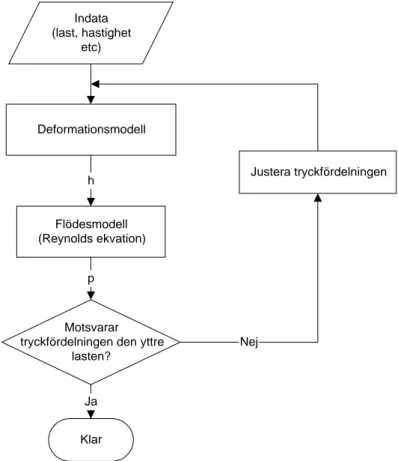
I princip använder ett EHD program tre samband för att lösa problemet. Ett samband mellan kropparnas deformation och kontakttrycket, en deformations-modell, också kallad filmtjockleksekvationen. Ett samband mellan geometri, ytornas hastigheter, smörjmedlets (vattnets) viskositet och trycket i kontakten, flödesmodellen som i detta fall är Reynolds ekvation. Slutligen används också sambandet mellan trycket i kontakten och den pålagda lasten. Schematiskt är beräkningsprogrammet beskrivet i figur 1. En mer detaljerad beskrivning finns också i bilaga 2 och 3. Bilaga 3 är utdrag från en presentation av projektets arbete med beräkningsprogrammet för att beräkna filmtjockleken under ett däck vid viskös vattenplaning. Justera tryckfördelningen Deformationsmodell Flödesmodell (Reynolds ekvation) h Indata (last, hastighet etc) Motsvarar tryckfördelningen den yttre

lasten? p

Ja

Nej

Klar

Figur 1 Schematisk beskrivning av simuleringsprogrammet

De problem som uppkommit hittills i arbetet med EHD programmet för mjuka material är främst av matematiskt beräkningsteknisk natur. Det är svårt att få programmet, som itererar sig fram till en lösning, att konvergera. Anledningarna är flera och finns bättre beskrivna i bilaga 2. En orsak till problemen är att små förändringar i kontakttrycket leder till stora deformationsändringar p.g.a. gummits låga E-modul. Detta gör lösningen instabil och en mängd numeriska knep måste införas för att beräkningarna ska konvergera.

Dessa numeriska knep är beskrivna i bilaga 2 och kommer i projektets nästa fas att införas i programmet för att avhjälpa konvergensproblemen. Därefter ska deformationsmodellen av det luftfyllda däcket, se kapitel 2, föras in i programmet vilket kanske kommer att leda till en del nya numeriska svårigheter. Tryckfördelningen under det belastade, luftfyllda däcket som vi kan se exempel på i bilaga 1, skiljer sig nämligen avsevärt från tryckfördelningen under en

(12)

VTI notat 9-2002 9

homogen gummikropp, se bilaga 3. I det luftfyllda däckets kontaktyta finns de högsta kontakttrycken vid däckets sidor medan det maximala kontakttrycket i kontakten mellan en homogen gummikropp och en slät yta ligger mitt i kontakten.

4 Projektets

fortsättning

Fram till nu har de båda delarna, däckets deformationsegenskaper och EHD beräkningsprogrammet, utvecklats separat. Nästa mål är att länka samman de båda delarna genom att föra in en förenklad beskrivning av däckets deformationer i EHD programmet.

EHD programmet behöver först kompletteras så att det fungerar väl för en solid gummikropp mot en stel slät yta. Ett av de stora problemen är att få de numeriska beräkningarna att konvergera mot en lösning, vilket också beskrivs i bilaga 2. När det väl är löst för en solid gummikropp återstår att få programmet att konvergera även med de speciella deformationsegenskaper som ett luftfyllt gummidäck har.

FEM programmet kan, som visas i bilaga 1, simulera deformationer och tryck för det släta modelldäcket. För att föra in dessa deformationsegenskaper i EHD programmet behövs en förenklad modell av däcket, kanske i form av en flexibili-tetsmatris som beskriver däckets deformationsegenskaper utifrån det statiskt deformerade tillståndet (den torra kontakten). Filmtjockleksekvationen (deforma-tionsmodellen i figur 1) består i det normala EHD fallet av tre delar, en konstant, den odeformerade geometrin och ett uttryck för de elastiska deformationerna som funktion av kontakttrycket (se även bilaga 2 och 3). Den odeformerade geometrin skulle för det luftfyllda däcket ersättas med den statiskt deformerade geometrin och de elastiska deformationerna skulle istället vara de små (linjärt) elastiska deformationstillskotten p.g.a. små ändringar i kontakttrycket.

Lyckas det att föra in det luftfyllda släta däckets deformationsegenskaper i EHD programmet för mjuka kontakter och att sedan få programmet att konvergera, så är projektets huvudmål nått. Då kan programmet beräkna vattenfilm och kontakttryck för ett visköst vattenplanande slätt däck och fungera som en verktygslåda vid studier av vattenplaning och våtfriktion.

5 Referenser

1. Moore D F: Friction and Wear in Rubbers and Tyres. Wear. Vol 61. No 3. pp 273-282. 1980.

2. Sinnamon J F & Tielking J T: Hydroplaning and Tread Pattern Hydrodynamics. UM-HSRI-PF-74-10. Highway Safety Research Institute. 1974.

3. Åström H: Elastohydrodynamiska aspekter på Vattenplaning - en litteratursammanställning. VTI notat 61-2001. Statens Väg- och transportforskningsinstitut. Linköping. 2001.

(13)

(14)

1 Modellering av bild ¨ack med finita

elementmetoden

Den finita elementmodell (FEM) som presenteras här har tagits fram för att skapa en förenklad de-formationsmodell av ett vanligt bildäck under statisk last. Däcket som simulerats är ett slätt 165 R15 PIARC testdäck p˚a en 41_/₂×15 fälg. Se Figur 1.2 för geometrin till däcket.

Den kommersiella programvaran ABAQUS har använts för beräkningarna som redovisas i denna bilaga. Däcket har modellerats med ett isotropiskt hyper- och viskoelastiskt gummimaterial i en-lighet med ett exempel fr˚an ABAQUS. St˚alarmeringen i däcket modelleras med ABAQUS-kommandot

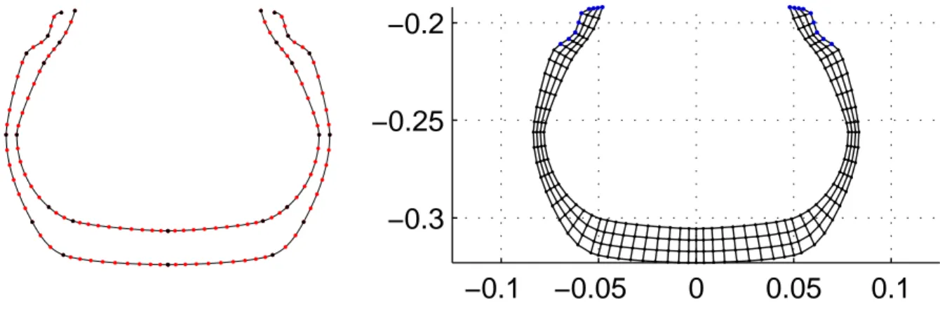
*REBARsom är gjort just för detta ändam˚al. Elementindelningen till FE-modellen skapas med pro-grammen MetaPost och Matlab, och illustreras i Figur 1.3. Sammantaget ger detta en mycket realistisk modell av ett bildäck.

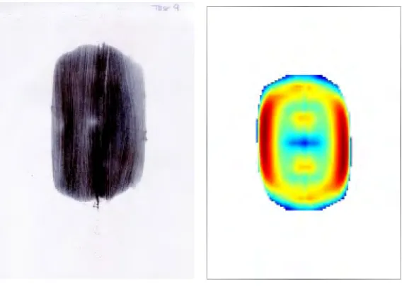
För att validera FE-modellen gjordes ett laboratorieförsök med ett riktigt PIARC testdäck. Däcket belastades i utrustningen Friktionsmätare BV-12 mot ett styvt underlag enligt Tabell 1.1. Lasten mättes med b˚ade BV-12:an och en v˚ag placerad under däcket. Kontaktarean mellan det belastade däcket och underlaget mättes med hjälp av ett tryckkänsligt grafitpulver (se Figur 1.5–1.16 (a)). Kontaktavtrycken lästes sedan in med en skanner och kontaktarean beräknades med ett Matlabprogram.

Motsvarande experiment utfördes i FEM-miljö. I FEM-programmet anlades först ett 200 kPa ringtryck. Sen belastades däcket mot en oändligt styv yta med en lastkontrollerad algoritm till samma niv˚aer som i laboratorieförsöket. Kontaktavtrycket erhölls genom att alla koordinater och kontakt-tryck för noderna i kontaktytorna exporterades till en resultatfil (se Figur 1.5–1.16 (b)). Kontaktarean beräknas automatiskt av ABAQUS. Se Figur 1.1 (a) för hela däckmodellen, och (b) för en detalj av en deformerade kontaktzonen.

I Figur 1.4 redovisas resultatet av b˚ade laboratorie- och FEM-försöket. Som synes blir det en väldigt bra överensstämmelse mellan teori och verklighet vilket borgar för att FE-modellen kan användas som en realistisk modell för hur ett riktigt bildäck p˚averkas av laster mellan, i alla fall, noll till 6 kN.

Tabell 1.1: Laboratorief¨ors¨ok med BV-12

Test nr. BV-12 Last [kN] V˚ag [Kg]

1 990 100 2 1928 195 3 2920 295 4 3890 390 5 4980 500 6 6420 640 7 5790 580 8 4750 475 9 3970 400 10 2940 295 11 1980 200 12 790 75 1 Bilaga 1

(15)

(a) FE-modell av PIARC testd¨ack. (b) Deformerad detalj.

Figur 1.1: FE-modell

Figur 1.2: Källa till geometrin för 165 R15 PIARC testdäck.

(16)

(a) D¨ackkontur fr˚an MetaPost.

−0.1

−0.05

0

0.05

0.1 −0.3

−0.25

−0.2

(b) Elementmesh fr˚an Matlab.

Figur 1.3: Generering av elementmesh med MetaPost och Matlab.

0 1000 2000 3000 4000 5000 6000 7000 0 0.5 1 1.5 2 2.5 3x 10 4 Kraft [kN] Kontaktarea [mm 2 ] Laboratorietest FEM−simulering

Figur 1.4: Jämförelse mellan laboratorieförsöket och FEM-simuleringen

(17)

(a) Laboratorietest. (b) FEM-simulering.

Figur 1.5: Kontaktarea vid 990 kN last.

(18)

(19)

(20)

(21)

(22)

(23)

(24)

Bilaga 2 Sida 1(10)

VTI notat 9-2002

EHL Aquaplaning - Initial Study: Elliptic Soft-EHL Contact Problem

by Alexei Jolkin 1. Background

Aquaplaning (called Hydroplaning in North America) occurs when water on the roadway accumulates in front of the vehicle's tires faster that the weight of the vehicle can push it out of the way. The water pressure can cause the car to rise up and slide on top of a thin layer of water between the tires and the road. While aquaplaning the vehicle rides on top of the water and can completely lose contact with the road, putting road-users in immediate danger of sliding out of the lane.

The following factors contribute to aquaplaning are:

• Vehicle speed. As speed increases, wet traction is considerably reduced. Aquaplaning can result in a complete loss of traction and vehicle control

• Vehicle weight - the lighter the vehicle, the more likely it is to hydroplane

• Road surface type - non-grooved asphalt is considerably more hydroplane-prone than ribbed or grooved concrete surfaces

• Water depth. The deeper the water, the sooner you will lose traction, although even thin water layers can cause a loss of traction, including at low speeds

• Tire size - the size and shape of a tire's contact patch has a direct influence on the probability of a hydroplane. The wider the contact patch is relative to its length, the higher the speed required supporting aquaplaning

• Tire treads depth. As the tires become worn, their ability to resist aquaplaning is reduced

• Tire tread pattern - certain tread patterns channel water more effectively, reducing the risk of aquaplaning

• Tire pressure

• Water composition (oil, temperature, dirt, & salt can change its properties and density) • Vehicle drive-train

Let's examine what happens to a tire in the midst of a hydroplane. When entering a puddle, the surface of the tire must moves the water out of the way in order for the tire to stay in contact with the pavement. The tire pushes some of the water to the sides, and forces the remaining water through the tire treads. On a smooth polished road in moderate rain at 90 km/h, each tire has to displace about four litres of water every second from beneath a contact patch no bigger than a palm of hand. Each gripping element of the tread is on the ground for only 1/150th of a second; during this time it must displace the bulk of the water, press through the remaining thin film, and then begin to grip the road surface.

With other words, water acts as a lubricant on rubber. This fact brings the car tire aquaplaning problem close to the lubrication problem of machine elements. The major difference of aquaplaning research is to increase friction and eliminate the water lubricating layer in order to improve traffic security, whereas the lubrication of machine components has its goals in reducing friction and wear by building a thick and stable lubricant film. The mathematical model is, however, very similar in both situations. The surfaces in the contact are deformed elastically and separated by a layer of lubricant, either oil or water. The separating film has a very complex shape formed by a lubricant (water) flow in a gap between the surfaces.

Due to complexity of the entire problem, a number of assumptions are used in the present initial study.

(25)

Bilaga 2 Sid 2 (10)

VTI notat 9-2002

• A system consisting of a single tire loaded against a perfectly smooth road surface is considered

• A bald perfectly smooth tire is assumed. Although bald tires give better grip on dry roads than treaded tires, they are unsafe in rain. However, they are extensively used in different kind of research.

• A very thin water film between the tire and the road is assumed, an assumption of the so-called viscous aquaplaning. No inertia effects are considered.

• The tire is considered as a homogeneous isotropic body of low elasticity modulus • Pure water lubrication is assumed

This model makes it possible to predict the contact pressure and the thickness of the separating water film under different circumstances, such as variable speed and load, sliding, etc.

2. Introduction

Fluid film lubrication occurs when opposing surfaces are completely separated by a lubricant

film that also carries the entire contact load. The subject of the present work is

Elastohydrodynamic lubrication (EHL) which is a mode of fluid film lubrication in which

high contact pressure causes elastic deformation of the contacting surfaces of much higher order of magnitude as the lubricant film separating them.

The earlier studies of elastohydrodynamic lubrication of elliptical conjunctions are applied to the particular and interesting situation when a car tire rolling on a wet surface. This situation exhibited by low-elastic modulus material leads to the so-called Soft EHL. The procedure used in obtaining the soft-EHL results which is described by a number of authors (see references [1], [2], [3], [4]) is applied in this study with minor modifications.

The objective of the work presented in this report is to develop a numerical method for the investigation of water-lubricated soft elastohydrodynamic conjunctions as it relates to the problem of car tire aquaplaning.

3. Governing equations

A mathematical model would allow the water film shape and pressures in the contact between the tire and the road to be determined and analysed. This model comprises the Reynolds equation, the film thickness equation and the force balance equation.

3.1 The Reynolds equation

Knowing the velocities of the surfaces and their geometry, we can calculate the pressures in the water film with Reynolds Equation:

(

) ( )

x h U U y p h y x p h x ∂ ∂ + =       ∂ ∂ ∂ ∂ +       ∂ ∂ ∂ ∂ ρ η ρ η ρ 2 1 3 3 6 (1)

where x and y are spatial coordinates along the direction of motion and in transverse direction respectively

p = p(x,y) is pressure in the contact

h = h(x,y) is function describing the separation between two interacted bodies (lubricant

film thickness)

ρ is the density of water

(26)

Bilaga 2 Sida 3(10)

VTI notat 9-2002

U1, U2 are surface velocities of the road and the tire respectively

The following common assumptions are considered in the present investigation: • Newtonian fluid • Iso-viscous fluid • Incompressible fluid • Steady-state • Isothermal • Smooth surfaces

• Fully flooded conditions

We need to satisfy the following boundary conditions:

at the inlet: p=0

on each side of the contact: p=0 (1a)

at the cavitation boundary: =0 ∂ ∂ = x p p

3.2 Film thickness equation

Irrespective of lubricant flow, rheological behaviour or thermal conditions, the film thickness in a two-dimensional EHL contact can be written as the sum of the undeformed gap geometry, and the elastic deformation of the surfaces:

) , ( ) , ( ) , (x y h00 g x y w x y h = + + (2)

where h(x,y) is the lubricant film thickness, g(x,y) the gap between the undistorted equivalent body surface and a touching plate, h00 is the film thickness at the origin of coordinates had the

surfaces been undistorted and w(x, y) is the actual elastic deformation of the equivalent body surface.

The limited extent of tire contact with the road makes it possible to assume that curves describing undistorted surface of car tire close to and within the boundaries of the region of pressure can be approximated by an elliptic torus, which can be seen in Figure 1.The elliptic toroidal shape is given by parametric equations:

( )

(

) ( )

( )

θ

(

( )

ϕ

)

ϕ θ ϕ cos cos sin sin cos a c a c z b y a c x + − + = = + = (3) where

a – semi-minor axis of ellipse b - semi-major axis of ellipse c - centre radius of torus ϕ∈ [0, 2π[

θ∈ [0, 2π[

However, parametric representation of the surfaces has its certain limitations. For given coordinates x and y Cartesian representation for the tire surface g(x,y) is used:

Figure 1. Elliptical torus in Cartesian coordinates

(27)

Bilaga 2 Sid 4 (10) VTI notat 9-2002

( )

(

ϕ

) ( )

θ ϕ θ ϕ cos cos ) , ( cos arcsin arcsin a c a c y x g a c x b y + − + =       + =       = (3a)

For two continuous bodies that are loaded against each other or separated by a thin water film, the total normal deflection w(x, y) from their undistorted shape can be written as an integral relationship:

(

) (

)

∫ ∫

+∞ ∞ − +∞ ∞ − ′ ′ ′ ′ ′ ′ = K x x y y p x y dxdy y x w( , ) , , , , (4)

where p(x,y) is the lubricant pressure acting over the contact between surfaces

The integral kernel K(x,x’,y,y’) of a contact problem may take different forms depending on each elastic system studied. A car tire is a rather complicated elastic system. To establish a general expression for the integral kernel of a loaded pressurised shell is the subject for further investigations.

The mathematical model used here is restricted by the following assumptions: • Car tire is a homogeneous, isotropic and perfectly elastic body

• A frictionless contact is assumed

These assumptions however do not affect generality of the numerical approach developed here.

In assumptions above, the total deflection w(x,y) of a car tire loaded against the road becomes:

∫ ∫

+∞ ∞ − +∞ ∞ − − ′ + − ′ ′ ′ ′ ′ ′ = 2 2 ) ( ) ( ) , ( 2 ) , ( y y x x y d x d y x p E y x w π (4a)

where E´ is the effective elastic modulus.

3.3 Force Balance equation

The force balance equation (5) imposes a global condition of equilibrium on the film thickness equation; the calculated load must be equal to the value F measured experimentally.

∫∫

Ω

= p x y dxdy

F ( , ) (5)

By altering h00 the whole pressure distribution is raised or lowered until it satisfies the force

balance equation, the film thickness equation and the Reynolds equation. 4. Discrete Equations

The equations are discretized on a rectangular uniform grid with mesh size hx and hy extended over the domain Ω,

{

a<y<b,c<x<d

}

. A second order accurate discretisation of the Poiseuille

terms and one-sided upstream second order discretisation of Couette term gives the following discrete Reynolds equation:

(28)

Bilaga 2 Sida 5(10) VTI notat 9-2002

(

)

(

) (

)

(

)

(

) (

)

x j i j i j i j i ij ij y j i j i ij ij j i ij j i j i j i ij x j i j i ij ij j i ij j i j i j i ij ij h h h h h p e e p e e e p e e h p e e p e e e p e e p L , 2 , 2 , 1 , 1 2 1 , 1 , 1 , 1 , 1 , 1 , 2 , 1 , 1 , 1 , 1 , 1 , 1 5 . 0 2 5 . 1 2 2 2 2 − − − − + + + − − − + + + − − − + − = = + + + + − + + + + + + − + ≡ ≡ ρ ρ ρ (6) where

(

)

ij ij ij ij U U h e η ρ 2 1 3 6 + =

Note, that this is a most general expression for the discrete Reynolds equations. In the assumptions above, ρ_ij =ρ≡const and η_ij =η≡const

Approximating the pressure profile by a piecewise constant function on a uniform grid with mesh size hx and hy and value pkl in the region

} 2 2 2 2 ) , {(x y ∈R2 xk−hx ≤x≤xk +hx ∧yl−hy ≤ y≤yl+hy ,

where p_kl = p(x_k,y_l), the elastic deformation (4a) at grid point (i,j) can be written as

kl n k n l ikjl ij j i D p E w y x w x y

∑∑

= = ′ ≈ = 1 1 2 ) , ( π (7)

The influence coefficients Dikjl are given by

(

)

(

)

∫

+ − + − − + − = 2 / 2 / 2 / 2 / '2 '2 ' ' x k x k y l y l h x h x h y h y _i _j ikjl y y x x dy dx D (8)

Analytically calculated coefficients Dikjl are given by the expression found by Love [40]:

        + + + + +         + + + + +         + + + + +         + + + + = ₂ ₂ 2 2 2 2 2 2 2 2 2 2 2 2 2 2 ln ln ln ln p m m p p p p p m p m m m m m p p m m m m m p m p p p p ikjl y x x y x x y y x y y x y x y x x y x x y y x y y x y x D where x_p =x_i−x_k+h_x/2, x_m=x_i−x_k−h_x/2, y_p =y_j−y_l+h_y/2, y_m= y_j−y_l−h_y/2 The discrete film thickness equation is finally written as:

kl n k n l hhhh ikjl ij ij D p E g h h x y

∑∑

= = ′ + + = 1 1 00 2 π (i=1..nx, j=1..ny) (9) The force balance equation is discretised in the same way as film thickness equation, i. e. approximating pressures by a piecewise constant function on a uniform grid with mesh size hx and hy:

∑∑

= = ≈ nx y i n j ij y xh p h F 1 1 (10) 4. Numerical approach

In order to design a stable and efficient relaxation scheme it is necessary to understand the nature of the equations. Due to elastic effects the coefficient e in equation (6) varies many orders of magnitude over the domain Ω. For large values of e the differential aspects as represented by the second order derivatives of the pressure determine the behaviour. For small values of e the ∂

( )

ρh ∂x term dominates the behaviour, and, because the film thickness equation is given by an integral equation, the problem behaves as an integral problem.

(29)

Bilaga 2 Sid 6 (10)

VTI notat 9-2002

Understanding how to solve this problem for large and small values of e forms the key to understanding how to construct an efficient solver for the complete EHL problem.

Generally speaking, the system of non-linear equations (6, 9, 10) consists of a very large number of unknowns. Any direct method to solve this problem is of questionable applicability. This difficulty can be overcome by using the approximate relaxation method. There are many different iterative processes and it goes beyond the scope of this investigation to give a detailed overview. Two very basic processes referred to as Jacobi and Gauss-Seidel relaxation respectively are often used in practice.

In words the process can be described as follows. Given an approximation to the solution of the problem in each grid point, a new approximation is computed by scanning the grid points in a prescribed order, changing the value in each grid point such that the local equation in this point is satisfied. The process comes in two flavours. If the new values are computed using only old values in the surrounding grid points it is referred to as Jacobi relaxation (Simultaneous Displacement). If the changes made when relaxing previous grid points are taken into account when relaxing the next grid point it is referred to as Gauss-Seidel relaxation (Successive Displacement). For Jacobi relaxation the order in which the grid points are relaxed is irrelevant. For Gauss-Seidel relaxation it makes a difference. Often the grid points are scanned in order to increasing grid indices in which case one refers to it as Gauss-Seidel relaxation with lexicographic ordering.

However, neither of the relaxation processes is suited to efficiently solve the problem for all values of e over the whole domain Ω. The Gauss-Seidel relaxation is an excellent method for large values of e but unstable for small e. On the other hand the distributive line Jacobi relaxation is a good method for very small e but rapidly looses efficiency with increasing e. The objective is to obtain an efficient solver. Let us introduce a parameter ξ. A good choice to obtain an efficient solver seems to be to use different relaxations for different grid points, as schematically shown in Figure 2. This figure presents a typical pressure and film thickness profiles in an elastohydrodynamically lubricated contact.

• On grid points where ξ/(hxhy) > ξlim the Gauss-Seidel line relaxation is used

• On grid points where ξ/(hxhy) ≤ ξlim the Jacobi distributive line relaxation is used

Where ξlim is a switch parameter to be defined. From practical tests i6t was found that an

efficient solver could be obtained using ξlim ≈ 0.3 and some underrelaxation in both the

processes. Typically ωJacobi = 0.6 and ωG.-S. = 0.8.

Low pressure Hydrodynamic effects prevail Line Gauss-Seidel Cavitation Line Gauss-Seidel High pressure Surface deformation is pre-dominant factor Distributive Jacobi Pressure Film thickness U1 U2

Figure 2. EHL conjunction. Schematic chart. Choice of relaxation scheme for different grid points

(30)

Bilaga 2 Sida 7(10)

VTI notat 9-2002

A line relaxation can be described as follows. Let ~pij denote the approximation to pij and

ij

h~ the associated approximation to hij. One relaxation sweep yelding an improved approximation pij and hij then consists of the following steps. The grid is scanned line by line, at each line applying changes to all the points of the line simultaneously, and, if distributive relaxation is used partly to the neighbouring lines. Subsequently, the new approximation pij can be used to obtain hij. For line relaxation in x-direction the changes δpij to be applied at given line j (and partly to the neighbouring lines) are solved from a system of equations of the form

ij s i k kj kj p r a =

∑

< − δ (11)

where rij is the vector of residuals and akj are the coefficients which exact definition depends on the type of the relaxation applied. For the described problem, the definition of rij and akj is given below. is given below. Theoretically, the matrix a is a full matrix. However, to obtain the line relaxation efficiency it is generally not needed to solve the system exactly. In practice it is often sufficient to take into account only the terms in the summations related to the direct neighbours of a point (i,j). This is justified because coefficients a decrease with increasing distance from the point (i,j). In particular it is sufficient to solve a three-diagonal system for Gauss-Seidel line relaxation and hexa-diagonal system for Jacobi distributive line relaxation.

4.1 Gauss-Seidel Line Relaxation

The discrete Reynolds equation at grid point (i,j) is given by equation (6). We sweep line by line in OX direction. The residual at the grid point (i,j) depends upon the given approximation

pij, pi-1,j, pi+1,j, expression (12):

(

)

(

)

(

)

(

)

(

)

(

) (

)

(

)

(

) (

)

2 1 , 1 , 1 , 1 , 1 , 1 , 2 , 1 , 1 , 1 , 1 , 1 , 1 , 2 , 2 , 2 , 1 , 1 , 1 , 1 , , 1 2 2 2 2 5 . 0 2 5 . 1 , , y j i j i ij ij j i ij j i j i j i ij x j i j i ij ij j i ij j i j i j i ij x j i j i j i j i j i j i ij ij ij j i j i j i ij h p e e p e e e p e e h p e e p e e e p e e h h h h h h h p p p r + + + − − − + + + − − − − − − − − − + − + + + + − + − + + + + − + − − ∆ + + ∆ + − ∆ + ≡ ρ ρ ρ with ∆ =

∑∑

l k lk ikjl ij D p h δ , ∆ ₋ =

∑∑

₋ l k lk kjl i j i D p h 1 1 δ and ∆ − =

∑∑

− l k lk kjl i j i D p h 2 2 δ (13)

The corrections of pressure δpij (note that δpij= 0 at first iteration) are solved from the linear three-diagonal system: ij j i j i j i j i j i j i p a p a p r

a₋1,δ ₋1, + ,δ , + ₊1,δ ₊1, = for each fixed j (14)

where coefficients

( )

ij ij ij ij p p r a ~ ∂ ∂ = are pre-computed:

(

)

x j i j i ij x j i ij j i ij j i h D D D h e e p r a ₂ 1, 10 1 00 2, 10 , 1 , 1 5 . 0 2 5 . 1 2 − − − − − + − − + = ∂ ∂ ≡ ρ ρ ρ

(

) (

)

x j i j i ij y j i ij ij x j i ij j i j i ij j i h D D D h e e e h e e e p r a 1 ₂ 1, 1 ₂ , 1 00 1 10 2, 20 , , 5 . 0 2 5 . 1 2 2 2 2 ₊ ₋ ₊ ₋ ₋ − + + ₋ + + ₋ − + − = ∂ ∂ ≡ ρ ρ ρ (15)

(

)

x j i j i ij x j i ij j i ij j i h D D D h e e p r a ₂ 1, 10 1 20 2, 30 , 1 , 1 5 . 0 2 5 . 1 2 − − + + + + − − + = ∂ ∂ ≡ ρ ρ ρ

(31)

Bilaga 2 Sid 8 (10)

VTI notat 9-2002

After all the pressure corrections δpij are calculated, a new approximation pij in each grid point is computed according to

ij S G ij ij p p p = +ω .− .δ (16)

The film thickness updates ∆hij are then calculated according to expressions (13) and applied in calculation of residuals at next relaxation sweep. A schematic chart of the Gauss-Seidel line relaxation is shown in Figure 3.

4.2 Jacobi Distributive Line Relaxation

A second order distributive Jacobi relaxation was applied here. This technique is described by many authors (see, for example, Brandt [2], Venner [4]). A grid point (i,j) is defined as a Jacobi distributive line relaxation point if ξ/(hxhy) ≤ ξlim. For such a point the residual at the

grid point (i,j) depends upon the given approximation on pij, pi-1,j, pi+1,j, (17):

(

)

(

)

(

) (

)

(

)

(

) (

)

2 1 , 1 , 1 , 1 , 1 , 1 , 2 , 1 , 1 , 1 , 1 , 1 , 1 , 2 , 2 , 1 , 1 , 1 , , 1 2 2 2 2 5 . 0 2 5 . 1 , , y j i j i ij ij j i ij j i j i j i ij x j i j i ij ij j i ij j i j i j i ij x j i j i j i j i ij ij j i j i j i ij h p e e p e e e p e e h p e e p e e e p e e h h h h p p p r + + + − − − + + + − − − − − − − + − + + + + − + − + + + + − + − − + − ≡ ρ ρ ρ

The corrections of pressure δpij are solved from the linear hexa-diagonal system:

ij j i j i j i j i j i j i j i j i j i j i j i j i p a p a p a p a p a p r

a₋3, δ ₋3, + ₋2,δ ₋2, + ₋1, δ ₋1, + ,δ , + ₊1, δ ₊1, + ₊2,δ ₊2, = for each fixed j (18)

where _       ∂ ∂ + ∂ ∂ + ∂ ∂ + ∂ ∂ − ∂ ∂ = + − + −1 1 1 1 4 1 ij ij ij ij j i ij j i ij ij ij ij p r p r p r p r p r

a for 1<i<ni and 1<j<nj

Let us introduce 4

{

1, 1, , 1 , 1

}

1 + − + − + + + − = ∆Dij Dij Di j Di j Dij Dij x j i j i ij j i h D D D a 3, 30 1 20 2, 10 5 . 0 2 5 . 1 ∆ − ∆ + ∆ − = − − − ρ ρ ρ For each line Pressure relaxation Building the system Solving the system

Updating the pressures

Film thickness calculation

(32)

Bilaga 2 Sida 9(10) VTI notat 9-2002

(

)

x j i j i ij x j i ij j i h D D D h e e a 2, ₂1, 20 1 10 2, 00 5 . 0 2 5 . 1 2 4 1 ∆ − ∆ + ∆ − + − = − − − − ρ ρ ρ

(

) (

)

x j i j i ij y j i ij j i x j i ij j i x j i ij j i h D D D h e e e h e e e h e e a 1, ₂1, 1, ₂ 1, , 1 ₂ , 1 10 1 00 2, 10 5 . 0 2 5 . 1 2 2 4 1 2 2 4 1 2 ∆ + ∆ − ∆ − + + + + + + + = − − + − + − − − ρ ρ ρ

(

) (

)

x j i j i ij y j i ij j i x j i ij j i j i h D D D h e e e h e e e a, 1, ₂ 1, , 1 ₂ , 1 00 1 10 2, 20 5 . 0 2 5 . 1 2 2 4 5 2 2 4 5 ∆ − ∆ + ∆ − + + − + + − = − + − + ρ ρ− ρ− (19)

(

) (

)

x j i j i ij y j i ij j i x j i ij j i x j i ij j i h D D D h e e e h e e e h e e a 1, ₂1, 1, ₂ 1, , 1 ₂ , 1 10 1 20 2, 30 5 . 0 2 5 . 1 2 2 4 1 2 2 4 1 2 ∆ + ∆ − ∆ − + + + + + + + = − − + − + − − + ρ ρ ρ

(

)

x j i j i ij x j i ij j i h D D D h e e a 2, ₂1, 20 1 30 2, 40 5 . 0 2 5 . 1 2 4 1 ∆ − ∆ + ∆ − + − = − − − + ρ ρ ρ

where Dii′jj′=Di−i′,j−j′ ≡Dkl, and i−i′=k and j− j′=l

Hexadiagonal system is solved using Gaussian elimination and subsequently the changes ij

p

δ are applied to the line j.

The changes are applied according to the scheme

          − − − − 0 1 0 1 4 1 0 1 0 4 1 ij δ

As a result of the distributive changes the new approximation pij to pij is given by:

{

( )

}

~ 1 , 1 , , 1 , 1 4 1 , − − + + + − + + + = ij Jacobi ij i j i j i j ij ij p p p p p p p ω δ δ δ δ δ (20)

After all the pressure corrections δpij are calculated, the pressure updates pij is calculated according to expression (20) and applied in calculation of film thickness at next relaxation sweep. A schematic chart of the Jacobi distributive line relaxation is shown in Figure 4.

The solution of the EHL problem is subject to a special condition, the cavitation condition 0

≥

p in Ω. This condition should be taken into account when constructing the system of equations to be solved in the relaxation. Also when applying the changes the cavitation condition must be taken into account. The procedure to apply the changes solved for the line j is the following. If a point (i,j) is a Gauss-Seidel point the change ωG.−S.δpij is applied. If the resulting pressure pij =pij+ωG.−S.δpij is smaller then zero it is set to zero. If the point (i,j) is a Jacobi distributive point the change ~

{

4( 1, 1, , 1 , 1)

}

1 , − − + + + − + + + = ij Jacobi i j i j i j ij ij ij p p p p p p p ω δ δ δ δ δ is applied

to the point (i,j). If the resulting pressure is smaller then zero it is set to zero. The net change, i.e. corrected for the cavitation condition, is then distributed to the neighbouring points according to the distribution. Finally, the change to the central point is always applied, however, the changes to the neighbouring points are only applied if the current pressure at these points is larger then zero and also, after these changes have been applied the cavitation condition p≥0 is imposed in these points.

(33)

Bilaga 2 Sid 10 (10)

VTI notat 9-2002

5. Concluding Remarks and Future work

A numerical algorithm for determining water separating films and pressures in the water-lubricated contact between a car tire and a road is developed in the present research. The reliable algorithm is developed to provide a stable solution to a highly non-linear viscous flow problem with elastic boundaries.

The following steps in studying the viscous aquaplaning problem are suggested here and are subject of future investigations.

Firstly, the described algorithm must certainly be implemented in a computer program. The numerical results should be obtained and verified.

The next step is an implementation of the Multigrid Technique to accelerate convergence rate compared to a straightforward relaxation process.

During the next step the whole complex mechanical structure of the vehicle tire must be taken into account.

Taking into account these high-order effects would make it possible to understand the mechanisms of viscous aquaplaning and study of dramatic loss of friction already with very thin water films.

References

1. Hamrock B.J. “Fundamentals of Fluid Film Lubrication”, McGraw-Hill, ISBN 0-07-025956-9

2. Brandt A., "Multigrid Techniques: 1984 Guide with applications to fluid dynamics", available as G.M.D.-Studien No. 85, from G.M.D.-F1T, Postfach 1240, D-5205, St. Augustin 1, Germany.

3. Lubrecht A.A., “The numerical solution of the elastohydrodynamically lubricated line- and point contact problem using multigrid techniques”, Ph.D. thesis, University of Twente, Enschede, The Netherlands, ISBN 90-9001583-3, 1987

4. Venner C.H., “Multilevel solution of the EHL line and point contact problems”, Ph.D. Thesis, University of Twente, Enschede, The Netherlands, ISBN 90-9003974-0, 1991

For each line

Pressure relaxation Building the system

Solving the system

Updating the pressures

Film thickness calculation

(34)

Bilaga 3 Sida 1 (7)

(35)

Bilaga 3 Sid 2 (7)

(36)

Bilaga 3 Sida 3 (7)

(37)