Compression of multi channel audio at low bit rates using the AMR-WB+ codec

Full text

(1)2005:134 CIV. MA S T ER’S T H E SI S. Compression of Multi Channel Audio at Low Bit Rates Using the AMR-WB+ Codec. LARS ABRAHAMSSON. MASTER OF SCIENCE PROGRAMME Technical Physics Luleå University of Technology Department of Mathematics. 2005:134 CIV • ISSN: 1402 - 1617 • ISRN: LTU - EX - - 05/134 - - SE.

(2) Compression of multi channel audio at low bit rates using the AMR-WB+ codec. Lars Abrahamsson.

(3) Abstract The purpose of this thesis work done at Ericsson Research in Lule˚ a was to investigate the possibilities of encoding 5.1 surround sound for low bit rates using the AMR-WB+ audio encoding technique. In the first phase of the work, investigations of the inter-channel dependencies were carried out, and the main tool used was Matlab. Several efforts were made aiming to reduce the total energy of the signal. This was done by decorrelating the sound channels using ordinary linear predictors. Decorrelation attempts were performed in the time domain as well as in the frequency domain. After decorrelating the channels, each channel was encoded in an individual bit rate using the mono mode of AMRWB+ with bit rates proportional to the relative energy content. However, listening tests combined with studies of the energy reduction achieved by decorrelations indicated that, for a given bit rate, there is in general no advantage decorrelating the signal compared to not doing so. The second phase of the thesis work mainly consisted of modifying the existent C code of the AMR-WB+ mono coder in order to suit it for 5.1 sound encoding and decoding. The goal was “the simplest possible”, an encoder that encoded each unmodified sound channel individually, distributing the bit rates over the channels aiming to keep the sums of the bit rates over the channels approximately constant over time. Opposed to the five “normal” sound channels, the encoding of the LFE (Low Frequency Element) was done in a specific way making use of this, compared to the other channels, somewhat constrained signal. Furthermore, the method of encoding high frequency sounds of AMR-WB+, the BWE (BandWidth Extension), needed to be modified at some extent. Finally, the third phase consisted mainly of evaluation of the product made and of making comparisons to competing low bit rate multi channel coders.. i.

(4) Sammanfattning Syftet med detta examensarbete som gjordes p˚ a Ericsson Research i Lule˚ a var att utreda m¨ ojligheterna att koda 5.1-kanalsljud f¨ or l˚ aga bittakter med hj¨ alp av ljudkodaren AMR-WB+. I arbetets f¨ orsta fas utreddes ljudkanalernas ¨ omsesidiga beroenden, och huvudverktyget var Matlab. Flera olika insatser gjordes i syfte att f¨ ors¨ oka reducera signalens totala energi. Dessa f¨ ors¨ ok innebar reduktion av korrelationerna ljudkanalerna emellan. Korrelationernas reduktioner ˚ astadkoms med hj¨ alp av vanliga linj¨ ara prediktorer. Korrelationsreduceringsf¨ ors¨ ok utf¨ ordes s˚ av¨ al i tidsdom¨ anen som i frekvensdom¨ anen. Efter att ha reducerat korrelationerna kanalerna emellan kodades varje kanal i en individuell bittakt genom att anv¨ anda AMR-WB+:s monol¨ age. Varje kanals bittakt var proportionellt relaterad till kanalens relativa energiinneh˚ all. Emellertid visade lyssningstest i kombination med studier av den av korrelationsminskningen uppn˚ adda energireduktionen att, f¨ or en given bittakt, ger det i allm¨ anhet ingen vinst att reducera korrelationerna i signalen i j¨ amf¨ orelse med att inte g¨ ora det. Arbetets andra fas bestod till st¨ orsta delen av att modifiera befintlig C-kod fr˚ an AMR-WB+:s monokodare. Syftet med modifikationerna var att anpassa kodaren till att kunna koda och avkoda 5.1 flerkanalojliga”, det vill s¨ aga en kodare som sljud. M˚ alet sattes till ”det enklast m¨ kodade varje or¨ ord ljudkanal individuellt, och f¨ ordelade bittakterna ¨ over kanalerna med avsikten att h˚ alla summan av bittakter, ¨ over kanalerna, approximativt konstant i tiden. Till skillnad fr˚ an de fem ”normala” ljudkanalerna, kodas l˚ agfrekvenselementet p˚ a ett speciellt s¨ att f¨ or att dra nytta av denna, i j¨ amf¨ orelse med de andra ljudkanalerna, n˚ agot begr¨ ansade kanal. Vidare beh¨ ovde BWE:n (BandWidth Extension), metoden vilken AMR-WB+ anv¨ ander f¨ or att koda h¨ ogfrekvensljud, modifieras i viss utstr¨ ackning. Slutligen bestod den tredje fasen huvudsakligen av utv¨ ardering av den framtagna kodaren samt att g¨ ora j¨ amf¨ orelser med konkurrerande l˚ agbittakts kodare av flerkanalsljud.. ii.

(5) Acknowledgements My supervisor at Ericsson Research has been Ingemar Johansson, who has been of great help thanks to his experience, helpfulness, easy manner and skill. The help of his spans of course all the work done, but the most critical part has been the C programming where his help has been a necessity. My experience of C programming was before this thesis work close to nonexistent. I have had a shorter optional C++ course at upper secondary technical school only that is all. Except Ingemar, people supporting me in writing this thesis are Tomas Frankilla at Ericsson Research – proof reading, and my sister ˚ Asa – giving me support regarding the English language. Technical aid concerning Scientific WorkPlace is received from Johan Dasht, PhD student at the mathematics department of Lule˚ a University of Technology. Furthermore, thanks go to Amelia Schulteis, a German acquaintance I met at CERN last summer, for the help of managing the X-Fig/Win-Fig and Pstoedit picture editing and conversion programs. I would also like to thank the rest of the staff at Ericsson that I have got help and inspiration from, the computer technicians at TietoEnator as well as my examiner at the university – Thomas Gunnarsson. Thomas Gunnarsson is prefect at the department of mathematics at Lule˚ a University of Technology.. iii.

(6) Contents Contents. iv. List of Figures. vi. List of Tables. ix. 1 Introduction 1.1 Background . 1.2 Applications . 1.3 Teaser . . . . 1.4 Outline of the. . . . . . . . . . . . . Thesis. . . . .. . . . .. . . . .. . . . .. . . . .. . . . .. . . . .. . . . .. . . . .. . . . .. . . . .. . . . .. . . . .. . . . .. . . . .. . . . .. . . . .. . . . .. . . . .. . . . .. . . . .. . . . .. . . . .. . . . .. . . . .. 2 The Problem. 1 1 1 1 2 3. 3 Brief Description of the mono coder of AMR-WB+ 3.1 Time Separation . . . . . . . . . . . . . . . . . . . . . 3.2 Pre-emphasis and LP Filtering . . . . . . . . . . . . . 3.3 Immitance Spectral Frequency (ISF) . . . . . . . . . . 3.4 The ACELP Coder . . . . . . . . . . . . . . . . . . . . 3.5 The TCX Coders . . . . . . . . . . . . . . . . . . . . . 3.6 BandWidth Extension (BWE) . . . . . . . . . . . . . 3.7 Internal Sample Frequency (ISF) modes . . . . . . . . 3.8 Available Bit Rates of the Coder . . . . . . . . . . . .. . . . . . . . .. . . . . . . . .. . . . . . . . .. . . . . . . . .. . . . . . . . .. . . . . . . . .. 4 4 5 6 7 9 13 15 15. 4 Feasibility Study 16 4.1 Background Information . . . . . . . . . . . . . . . . . . . . . . . 16 4.2 The Matlab Simulations . . . . . . . . . . . . . . . . . . . . . . . 17 4.2.1 Introduction . . . . . . . . . . . . . . . . . . . . . . . . . 17 4.2.2 Band Splitting in the Time Domain . . . . . . . . . . . . 19 4.2.3 Recombination of the Split Signal . . . . . . . . . . . . . 22 4.2.4 Creation of Sum and Difference Channels . . . . . . . . . 22 4.2.5 Different Dependency Chains . . . . . . . . . . . . . . . . 24 4.2.6 Time Windowing . . . . . . . . . . . . . . . . . . . . . . . 24 4.2.7 Time Domain Decorrelation . . . . . . . . . . . . . . . . . 26 4.2.8 Time Domain Reconstruction . . . . . . . . . . . . . . . . 29 4.2.9 Two Smaller Dependency Chains . . . . . . . . . . . . . . 31 4.2.10 Additional Ideas Regarding the Decorrelation Efforts Made in the Time Domain . . . . . . . . . . . . . . . . . . . . . 33 4.2.11 Frequency Domain Decorrelation . . . . . . . . . . . . . . 34 4.2.12 Examples of FFT Domain Decorrelation . . . . . . . . . . 38 4.2.13 Bit Rate Allocation and Reference Channel Puzzles . . . 43 4.2.14 FFT Domain Reconstruction . . . . . . . . . . . . . . . . 44 4.2.15 Experiments Using the HF Part of the Front Channels in the Rear Channels as Well . . . . . . . . . . . . . . . . . . 44 iv.

(7) 4.3. 4.4 4.5. 4.2.16 FFT Domain Results . . . . . . . . . . . . . . . . . . . . . Modifications of AMR-WB+ needed to be made . . . . . . . . . 4.3.1 Introduction . . . . . . . . . . . . . . . . . . . . . . . . . 4.3.2 The Bass Channel, Also Known as the Low Frequency Element (LFE) . . . . . . . . . . . . . . . . . . . . . . . . 4.3.3 The Addition of Six Extra Low Bit Rate (TCX) Modes . 4.3.4 BandWidth Extension (BWE) . . . . . . . . . . . . . . . 4.3.5 The Noise-fill Feature of the Decoder . . . . . . . . . . . . Bit Rate Allocation . . . . . . . . . . . . . . . . . . . . . . . . . . Conclusions . . . . . . . . . . . . . . . . . . . . . . . . . . . . . .. 46 46 46 47 48 49 49 53 59. 5 Comparisons. 60. 6 Conclusions. 61. 7 Discussions 7.1 Making Use of the Existence of “Cheap” Surround . . . . . . . 7.2 Improving the Bit Rate Allocation Ideas . . . . . . . . . . . . . 7.3 Alternative Ways of Reducing the Inter-Channel Dependencies 7.4 The Usage of Sum/Difference Channels . . . . . . . . . . . . .. . . . .. 8 Future Work. 62 62 62 62 63 63. A Theoretical Background A.1 Basic statistics . . . . . . . . . . . A.1.1 One stochastic variable . . A.1.2 Two stochastic variables . . A.1.3 Several stochastic variables A.2 Energy . . . . . . . . . . . . . . . . A.3 SNR . . . . . . . . . . . . . . . . . A.4 Linear Prediction . . . . . . . . . . References. . . . . . . .. . . . . . . .. . . . . . . .. . . . . . . .. . . . . . . .. . . . . . . .. . . . . . . .. . . . . . . .. . . . . . . .. . . . . . . .. . . . . . . .. . . . . . . .. . . . . . . .. . . . . . . .. . . . . . . .. . . . . . . .. . . . . . . .. 64 64 64 65 66 67 67 67 73. v.

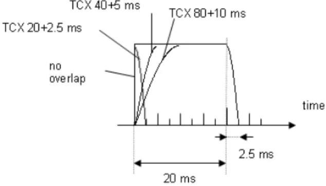
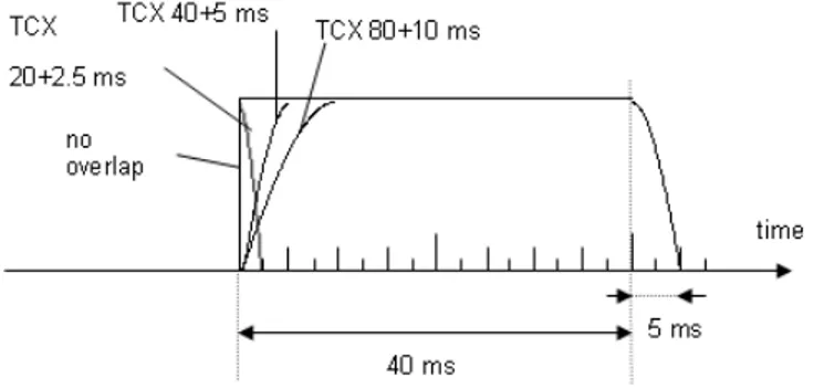
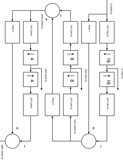
(8) List of Figures 1 2 3 4 5 6 7 8 9 10. 11. 12 13. 14 15. An outline describing the duration in time as well as stating the allowed positions of each coding mode within a “super frame”. . In this diagram, one can get a descriptive picture of how an ACELP encoder is working. The decoder is described in figure 3 In this diagram, one can get a descriptive picture of how an ACELP decoder is working. The encoder is described in figure 2. A figure that is briefly describing the principles of the TCX coding mode of AMR-WB+. . . . . . . . . . . . . . . . . . . . . . . . . . A visualization of the time window when using the coding mode TCX20. . . . . . . . . . . . . . . . . . . . . . . . . . . . . . . . . A visualization of the time window when using the coding mode TCX40. . . . . . . . . . . . . . . . . . . . . . . . . . . . . . . . . A visualization of the time window when using the coding mode TCX80. . . . . . . . . . . . . . . . . . . . . . . . . . . . . . . . . The spectrum of the original signal, as it looks before coding with the BandWidth Extension. . . . . . . . . . . . . . . . . . . . . . The spectrum of the signal plotted after folding the low frequencies over the break frequency all the way up to f2s . . . . . . . . . The spectrum of the signal as it looks after finalizing the BWE. The stored envelope of the HF part of the signal is now applied. Still, the fine structure of the HF part of the spectrum is replaced by the fine structure of the over folded parts of the LF spectrum. Figure illustrating the phenomenon that the narrower the bandwidth of a signal the slower the decay in the time domain is. The first row contains plots in the FFT domain while the second row contains plots in the time domain. Column one illustrates a narrowbanded signal, when at the same time column two illustrates a somewhat more broadbanded signal. . . . . . . . . . . . . . . . Band splitting process described as it was performed in the time domain. . . . . . . . . . . . . . . . . . . . . . . . . . . . . . . . . Recombination of the former separated and eventually processed frequency bands. The recombination is performed within the time domain. . . . . . . . . . . . . . . . . . . . . . . . . . . . . . The time window w(t), where π2 ≈ 1.57 corresponds to 10 ms. . . Diagram describing decorrelation of the channels as performed in the time domain. The C channel is leading; the remaining channels are dependent in a chainlike structure. The “Coder” blocks are representing both encoding and thereafter decoding of the encoded signal. The labels on the decorrelating filters tell the following. The first row; a predicts F S, b predicts F D, c predicts RS and d predicts RD. On the second row of the labels of the filters one can read which sound channel that is used for decorrelation. . . . . . . . . . . . . . . . . . . . . . . . . . . . . .. vi. 5 8 9 11 11 12 12 13 14. 14. 18 21. 22 26. 28.

(9) 16. 17 18. 19. 20. 21. 22. 23. 24. Reconstruction of each channel of the signal by adding the decorrelated channel to filtered versions of the channels it is depending ˜ F S means F g upon. Please note that C actually means C, S and so forth. This aesthetical and pedagogical inconvenience is due to technical limitations in the graphical software used (Dia). . . . The alternative decorrelation model, based on assumption of looser relations the front and back channels in between. . . . . . . . . . Decorrelation of the channels as it was done in the frequency domain. Note that the “Coder” blocks represent both encoding and decoding of the signal. Also note that the “Transmission” arrows are supposed to contain the encoded but yet not decoded signal. The latter remark is quite logical, though the sketch might be ambiguous to an outsider to the problem formulation. The figure is split into two pieces, where this is the first one and figure 19 is the second one. . . . . . . . . . . . . . . . . . . . . . The figure is split into two pieces, where this is the second one and figure 18 is the first one. In the caption text of the first one the description can be found. . . . . . . . . . . . . . . . . . . . . An example of a clip from Chapter 20 of the motion picture Pearl Harbour that is decorrelated. The decorrelations were performed in the frequency domain (0 − 6 kHz), with one real valued predictor for each leading channel and band. The amount of linear dependencies the channels in between of this illustration is quite representative for most of the signals used in the simulations. . . Decorrelating example (Roy Orbison – Only the Lonely) performed in the frequency domain (0 − 6 kHz), one real valued predictor for each leading channel and band. . . . . . . . . . . . An example of a short clip out of Roy Orbison – “Only the Lonely” decorrelated in a more sophisticated way. The decorrelations were performed in the frequency domain (0 − 6 kHz). Here, one predictor is used separately for the real and imaginary parts of each leading channel and band respectively. . . . . . . . Decorrelating example of a short clip out of Roy Orbison - “Only the Lonely” performed in the frequency domain (0 − 6 kHz). In this case, two predictors are used for each leading channel and band. One predictor is used for the real, and one is used for the imaginary part. Naturally, the real and imaginary parts of a depending channel have different predictors. This gives four predictors for each pair of channels. . . . . . . . . . . . . . . . . . An example of the not-so-well-working ideas of replacing the FFT coefficients of higher frequencies of the rear channels with coefficients of the front channels. In this example F S and F D are used. The case is quite similar when using the C channel instead.. vii. 30 32. 36. 37. 39. 40. 41. 42. 45.

(10) 25. 26. 27. 28. 29. A comprehensive sketch of how the “noise-fill” is implemented. Scrutinizing spectators might find several misleads and/or contradictions. Nevertheless, this draft is supposed to serve as a nice simplification – no more, no less. Black colour indicates spectral holes that are filled with noise. Discussions will be found in the sub subsection of “The Noise-fill Feature of the Decoder”. . . . . Example of bit rate allocation for a desired total bit rate of 80 kbps using the energy proportional bit rate allocation method. The graph of each channel is evened out by a 10 frames moving average filter. This is a clip out of Roy Orbison’s “Only the Lonely”, on the DVD album “A Black and White Night”. . . . . Example of bit rate allocation for a desired total bit rate of 80 kbps using the logarithmic energy proportional bit rate allocation method. The graph of each channel is evened out by a 10 frames moving average filter. This is a clip out of Roy Orbison’s “Only the Lonely”, on the DVD album “A Black and White Night”. . . Example of bit rate allocation for a desired total bit rate of 80 kbps using the energy proportional bit rate allocation method. The graph of each channel is evened out by a 10 frames moving average filter. This is a clip out of chapter 20 in the motion picture “Pearl Harbor”. . . . . . . . . . . . . . . . . . . . . . . . Example of bit rate allocation for a desired total bit rate of 80 kbps using the logarithmic energy proportional bit rate allocation method. The graph of each channel is evened out by a 10 frames moving average filter. This is a clip out of chapter 20 in the motion picture “Pearl Harbor”. . . . . . . . . . . . . . . . . . . .. viii. 52. 55. 56. 57. 58.

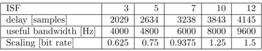
(11) List of Tables 1 2. The ISF-modes. . . . . . . . . . . . . . . . . . . . . . . . . . . . . The bit rates of the multi channel mode of AMR-WB+. . . . . .. ix. 15 15.

(12) 1 1.1. Introduction Background. In these days the multi-channel sound systems are getting of greater importance. The most common multi-channel setup is the 5.1 system with five “ordinary” sound channels; front left, front right, centre, rear left, rear right (from now on referred to as F L, F R, C, RL and RR) and one bass channel (from now on referred to as the low frequency element, the LF E). There are also other surround standards like 4.1, 6.1, and 7.1 with configurations in similar manners. As a matter of fact there are even standards with more than one LF E. Even though the human auditory system is bad at localizing low frequent (LF) sound sources, enthusiasts argue that several LF sources are needed for phenomenon like for example sound cancelling. The audio codec AMR-WB+ used in this thesis work originates from a speech coder named AMR, that originally was developed for GSM (Global System for Mobile Communications, a digital mobile phone system seen as a second generation system). AMR-WB+ (Adaptive Multi Rate - WideBand +) is a low bit rate wide-band sound encoder/decoder developed in co-operation by Ericsson, Nokia and VoiceAge.. 1.2. Applications. At the moment there is no known application for the multi-channel mode of AMR-WB+. On the other hand there is no reason for an audio coder of today not to have such a mode. One imagined application could be using the multi-channel mode of the coder for surround music in cars. Just docking the cellular phone to the car audio system and the music will start streaming from a server/radio station out in the loudspeakers. Anyway, a proper application needs to be mobile in some way. For a stationary receiver of audio there is nothing vindicating bit rates as low as those of AMR-WB+. Furthermore the receiving entity (vehicle) needs to be big enough for placing five to six speakers.. 1.3. Teaser. The subject of this thesis was to investigate whether or not it was possible to make a multi-channel coder suitable for all kinds of audio using the mono mode of AMR-WB+. If the answer to the first question was in the affirmative, such a coder would be constructed if there was time for it. This was the case, and a coder is constructed. This thesis is describing the investigations as well as the modifications of the audio coder that needed to be done. The first step in the is-it-possible-process was to investigate how great the linear dependencies the sound channels in between were for general 5.1 recordings. Somewhat surprising, the dependencies were close to nonexistent in most of the tested recordings. If there would have been more pronounced correlations. 1.

(13) those would have been used in order to decorrelate the channels. Decorrelation will in turn lead to energy reduction of the sound channels, and less energy of a signal will make it easier to encode in a lower bit rate with the amount of distortion unchanged. Since the correlations were small, the model used in the multi-channel encoder was the simplest possible. For a desired total bit rate, each sound channel was encoded individually by the mono coder in a bit rate such that when adding all the individual bit rates up the sum will equal the desired value. Two different ways of distributing the bit rate were tried out – both of them related the bit rate to the ratio between the energy of the channel in question and the total energy of all the channels. For each time frame the bit rate is redistributed. Changes that had to be made in the C code can be read about in detail further down in this thesis. One of the more important changes is that the LF parts of all the music channels but the centre channel is encoded on sums and differences of the front and rear channels instead of the original configuration of left/right channels. The HF parts of the same channels were on the other hand encoded using the original channel configuration. The bass channel is encoded in a special way that also is described in the thesis together with the rest of the things left out of this teaser. In order to determine if a sound coder is working well, listening tests are inevitable – just measuring and simulating can never replace the human ear. All listening tests have been performed in the purposely built, sound insulated, listening room at the facility of Ericsson Research in Lule˚ a. For an unaccustomed test listener, making judgements of which of two distorted sound clips that sounds “best” in some criteria can be quite challenging. My supervisor at Ericsson Research, Ingemar Johansson and his colleague Daniel Enström have been giving me lots of valuable help listening, and making relevant conclusions and judgements about the outcome.. 1.4. Outline of the Thesis. As the reader already may have noticed this is a part of the second chapter. The first chapter is acknowledgements. The third chapter gives an overview of the problem to solve. In the fourth chapter the encoder/decoder package is described. The biggest chapter, the fifth is split into five pieces. First some brief background information that is gathered by reading as well as by experimental work. In the second part, the Matlab simulations done are described and that is followed by a description of the changes done to the coder. Motivations to why the changes were done are included. The fourth part describes the ideas behind the bit rate allocation methods that were used. This part is presented separately because these ideas were used both in the Matlab simulations and in the C program that constitutes the coder. And finally the chapter is concluded with the fifth part containing some conclusions made regarding all these things. The sixth chapter is containing comparisons between the surround mode of WMA and the AMR-WB+ 5.1 coder of “ours”. That is followed by the seventh 2.

(14) chapter containing conclusions of the entire work done. In the eighth chapter, a very short bullet list of possible future improvements is presented. In chapter nine some of those ideas are shortly discussed. There are also one appendix chapter, A, which treats some theory needed for understanding and/or making it possible aping the work done for this thesis. Lastly written references used are listed.. 2. The Problem. The aim of this work was to, by the help of the mono coder of AMR-WB+, encode multi-channel audio of all kinds at bit rates as low as 48 − 64 kbps. Of course, at bit rates like these, one has to expect distortions to some extent. Nevertheless the sound needs to be at quality levels high enough not to be classified as psychological torture – and that’s the great challenge. Considering music sound, in some cases much higher bit rates are demanded than for other kinds of audio. What makes music harder to encode in general, compared to for example a movie, is that in a movie it is quite seldom that all sound sources produces relevant sounds at the same moment in time. And less speakers used implies less total amount of data to transmit. In a piece of music on the other hand, at least in recordings where the listener is supposed to be in the middle of the orchestra somewhere, there can be loud and relevant sounds in all the loudspeakers instantly. The target of 48 − 64 kbps can be compared to DTS and Dolby Digital, the two existing DVD audio standards for 5.1 audio. Usually the Dolby Digital 5.1 audio for 16 bit sound sampled at 48 kHz is encoded in a bit rate of 384 kbps. However, the Dolby Digital standard handles a variety of bit rates ranging all the way from 64 up to 448 kbps [Dolby]. Compared to DTS (Digital Theater Systems), the other DVD audio standard, Dolby Digital is quite destructively encoded. For home use, DTS is encoded in bit rates of approximately 800 kbps or somewhat less [DTS]. Two other surround sound standards more appropriate for home use are Fraunhofer’s “MP3 Surround” and Microsoft’s WMA format. These have been studied and evaluated. A more detailed comparison between the 80 and 128 kbps modes of the in this thesis work constructed coder and the 128 kbps mode of multi-channel WMA audio has been done as well. The interested reader will find more about this in 5. One main problem was examining if and how to make benefit of the statistic correlations between the sound channels of general 5.1 multi-channel audio. By the term “general”, different kinds of movies, live- and studio mixed music (not just music mixed by a certain method for example) are considered. The idea was that if some dependency the sound channels in between were found to be present, it could be of benefit for the coding. The total energy of the channels could be reduced if it was possible decorrelating them. Reduction of the energy of a sound channel would make it possible to encode the sound of that channel at significantly lower bit rates without increasing the experienced 3.

(15) distortion of the sound. In order to make use of the encoded decorrelated signal, of course parameters specifying the dependencies the channels in between need to be stored, quantized, and transmitted to the receiver of the signal. Thereafter the receiver can decode the decorrelated signal and finally recorrelate it using the transmitted parameters.. 3. Brief Description of the mono coder of AMRWB+. The focus of this work was not about digging deep in to the details of the wide band coder, it was rather more about usage and making necessary modifications of the coder. Anyhow it never hurts to have a rough idea about how it works, and at least some knowledge is a necessity. Therefore, this section is dedicated to a collection of descriptions that altogether gives a comprehensive overview of how the coder works.. 3.1. Time Separation. The coder is working in time frames of 20 ms. In order to be exact – these time 20 frames are actually scaling ms, where the scaling factor is ISF-mode dependent. Which factors that exist and what ISF mode they correspond to can be found in table 1. This is the explanation to why the same kind of time frames are used in the Matlab simulations that are to be described further down in this thesis. Each four time frames are grouped together in so called “super frames” with lengths of 80 ms. These super frames can be coded either as four 20 ms segments, two 40 ms segments, one 40 ms segment and two adjacent 20 ms segments, or simply as one entity of 80 ms. For each of these lengths there is one special coding mode; that is TCX80, TCX40 and TCX20. All the TCX coders are working in the (Fourier) transform domain. The number at the end of the name of each TCX coder mode tells the duration of the segment it is designed for. Or, in order to be exact, these are the durations of the segment excluding the for transform coders inevitable lookaheads. A lookahead is in AMR-WB+ 2.5 ms for each 20 ms of length of the time segment processed. In the 20 ms case there is also another, optional, coding mode which is called ACELP. ACELP is a time domain coding mode that does not use lookaheads. For clarifying purposes, an illustration of the allowed positions and time consumptions of each coding mode is stated in figure 1. The origin of this picture is [26.290]. The lookaheads also known as overlap and add, are here used in the purpose of avoiding “block artefacts”. That means avoiding discontinuities of the sound waveforms in the transitions between adjacent time frames. Which coding method to choose is determined by encoding the sound in all possible ways, computing the segmental SNR:s of each combination, and finally selecting the combination resulting in the highest on average segmental SNR. A segmental SNR is in this particular case an SNR that is computed for the time 4.

(16) segment of a 5 ms sub frame. The averages are computed over 4, 8 or 16 such sub frames depending on the length of the segment.. Figure 1: An outline describing the duration in time as well as stating the allowed positions of each coding mode within a “super frame”.. 3.2. Pre-emphasis and LP Filtering. Before the coding of the signal can take place, some pre-processing of it needs to be done. Firstly, pre-emphasis of the signal is done. The incoming mono signal is high pass filtered with a break frequency of the filter at 20 Hz. Thereafter, a first order filter h [n] = =. {h0 , h1 }. (1). {1, −0.68}. or, expressed in the Z-transform [Beta] domain H (z) = =. h0 + h1 · z −1 1 − 0.68 · z −1 5. (2).

(17) is applied to the signal. This altogether lowers the energies of the lower frequencies and raises the higher frequency energies of the signal. In turn, this procedure will enhance the resolution of the LPC analysis that is to come. A remark is at place here, in the decoding of the signal, naturally an inversion of the filter of equations 1 (time domain), 2 (Z-transform domain) is applied to the received and decoded signal. As hinted above, secondly, there is the LPC (Linear Predictive Coding) analysis to come, where a linear predictive filter is created. LPC is a method that lets the value of a signal each sample time be predicted linearly by the quantized values of the preceding samples. As a result the peaks in the spectrum of the error signal out of the LPC predictor will be restrained compared to the original signal. This resulting flatter spectrum, in turn, makes it easier to code the signal for the TCX and ACELP coders mentioned earlier. After the creation of the LP coefficients they need to be quantized. In case of data losses on the receiving side, the coefficients are interpolated from the properly reconstructed coefficients adjacent in time to the lost/corrupted one. There is one hook though. Neither quantization of, nor interpolation between time frames of, the polynomial coefficients ai of A (z) in formula 3, which is representing the previously determined LP filter, can normally be done without risking unstable or badly serving filters. Therefore, both the quantization and interpolation are performed in the ISF (Immitance Spectral Frequency) domain. The ideas behind will briefly be explained in the following.. 3.3. Immitance Spectral Frequency (ISF). The sensitivity for disturbances of the values of the polynomial coefficients of the filter of equation 3 is too high. Therefore, transforming the filters to a safer way of expressing them, namely into the ISF domain, is the solution. If the original LP filter is expressed as, A (z) = 1 +. N X. ai z −i. (3). i=1. that is the Z-transform [Beta] of the sequence of numbers {1, a1 , a2 , ..., aN } that constitutes the LP filter, then one can split up A (z) into the two polynomials P (z) and Q (z). These polynomials look like ¡ ¢ P (z) = A (z) + z −(N +1) A z −1 (4) ¡ −1 ¢ −(N +1) Q (z) = A (z) − z A z and add up to A (z) after dividing the created sum by 2 [LSP]. Each root of the polynomials P (z) and Q (z) have modulus one and they are alternating each other all around the unit circle; one root from P (z), one from Q (z), one from P (z), and so forth. Nevertheless, quantization of, and interpolation between time frames of, the roots of P (z) and Q (z) is easily done without the risks associated to working on the coefficients of A (z) directly. Furthermore, two 6.

(18) roots of Q (z) are all the time known to be −1 and 1 [26.190]. These two roots will consequently not need any quantization, storage or transmission. Please note that in theory, there is no stopping us from working with the roots of A (z) either, stability and disturbance sensitivity concerned. On the other hand, finding the roots of polynomials of degree > 4 must be done numerically in general. The process of finding a root of A (z) is considerably more complex than finding the roots of P (z) and Q (z), on which there are so many constraints. All these constraints, that are limiting the possible solutions of P (z) = 0 and Q (z) = 0 to the unit circle, and are letting one know that every other solution belongs to P (z) and Q (z) respectively, simplifies the iteration of root findings significantly. The polynomial coefficients of P (z) or Q (z) is not more or less sensitive to disturbances than the coefficients of A (z) in general – the thing is that finding the roots of the two former polynomials is easier than finding the roots of the latter one.. 3.4. The ACELP Coder. The ACELP (Algebraic Code Excited Linear Prediction [ACELP]) coding consists of LTP (Long Time Prediction, also known as ACB (Adaptive CodeBook)) analysis and synthesis, and algebraic codebook excitation. It is a predictive (from prior samples) encoder that is working in the time-domain. The ACELP coding mode is best suited for ordinary speech, sounds with one voice, single tones and transient sounds. Transients like snaps, or when speaking – consonants, are referred to. The ACELP mode of AMR-WB+ uses the same technique as the older AMR-WB speech coder, which AMR-WB+ is a kind of extension of. The diagram of figure 2 illustrates the concept of an ACELP encoder. The incoming sound is first filtered by a weighting filter, A (z) ³ ´ A γz. (5). ³ ´ where A (z) is the LP filter and A γz is the same LP filter but perceptually weighted by the 0 < γ ≤ 1 weighting factor. The purpose of the weighting filter is to move the coding noise to the parts in the frequency range where the ear is less sensitive, that is in the formant regions (the frequency regions in which it is the easiest to hide the noise). An attempt explaining the above written statement will follow. Quantization noise is in general almost white – that is, in terms of frequencies – evenly distributed all over the spectral range. However for parts of the sound with low energy, the noise energy might be so high that the useful parts of the sound will drown. This will in turn result in an unsatisfactory sound reproduction. There is one remedy though, the weighting filter of equation 5 recently described. Weighting in this case means that, keeping the energy of the noise constant, the energy distribution of the noise over the frequencies is modified. After 7.

(19) Input A(z)/A(z/gamma). ACB. g1. -. +. -. +. 1/A(z/gamma). +. e1. +. FCB. g2. 1/A(z/gamma). e2. Figure 2: In this diagram, one can get a descriptive picture of how an ACELP encoder is working. The decoder is described in figure 3 weighting, the noise energy is made small for small energies of useful sound, and vice versa. This means that, ideally, depending on the energies of the noise and of the useful sound, all the time the useful sound is supposed to drown the noise in a manner that would make it next to impossible to notice the noise for the average listener. Moreover, the mean square error (MSE) of the first “error-signal”, e1, is minimized by choosing the best available g1 scaling factor. The ACB block represents the Adaptive CodeBook. There is also a second “error-signal”, e2, whose MSE is minimized as well. The latter minimization process is embodied by choosing the optimal available g2 coefficient value. Inputs to the g2 scaling factor are codes coming out of the FCB block, the Fixed CodeBook. Please note that e1 and e2 are mutually dependent on each other due to the feedback of the system. The final error signal e2 is approximately the difference between Input of figure 2 and Output of figure 3. Note that the only data transmitted when using an ACELP coder is the g1, and g2 coefficients as well as the indices telling which code to use from the ACB and FCB code books. ACELP is a parameter based coder where the residual signals are not transmitted, just minimized in order to minimize the coding distortion.. 8.

(20) ACB. g1. +. Output 1/A(z). +. FCB. g2. Figure 3: In this diagram, one can get a descriptive picture of how an ACELP decoder is working. The encoder is described in figure 2.. 3.5. The TCX Coders. TCX is an acronym for Transform Coding eXcitation, and as the sound implies it is a transform coder. In TCX mode the perceptually weighted signal is processed in the transform domain. The Fourier transformed and weighted signal is quantized using split multi-rate lattice quantization. For deeper theoretical details about the transform coder, the reader is encouraged to consult [26.290]. Unlike the “old good” speech coder AMR-WB, AMR-WB+ is a coder appropriate for music as well as for speech. Consequently the encoding of music-like samples is what the “new” model, TCX, is best suited for. The complex valued Fourier coefficients are grouped four by four, represented as eight-dimensional real valued sub vectors. In total, there are 36, 72 and 144 of these sub vectors for the coding modes TCX20, TCX40 and TCX80 respectively. A figure describing the TCX coding can be found in figure 4. Here, one can first see³how ´ the input signal is processed by the perceptually weighted LPC z filter A γ , where γ is the weighting coefficient. Thereafter the pre-emphasis filter described earlier is applied. Windowing of the signal is done twice, first, before Fourier transforming the time signal, and second, after inverse transformation (see figure 4). The time window is defined as the concatenation of the three following sub windows ¶ µ 2π · n , n = {0, ..., L1 − 1} (6) w1 [n] = sin 4 · L1 w2 [n] = 1, n = {0, ..., L − L1 − 1} µ ¶ 2π · n w3 [n] = sin , n = {L2 , ..., 2L2 − 1} 4 · L1. 9.

(21) where L1 = 0 L1 = 32 L1 = 64 L1 = 128 L = 256 L2 = 32 L = 512 L2 = 64 L = 1024 L2 = 128. when the previous when the previous when the previous when the previous For 20-ms TCX For 20-ms TCX For 40-ms TCX For 40-ms TCX For 80-ms TCX For 80-ms TCX. frame frame frame frame. is is is is. a 20-ms ACELP frame a 20-ms TCX frame a 40-ms TCX frame an 80-ms TCX frame (7). and this can be somewhat further clarified by the three figures 5, 6 and 7 originally found in the document of [26.290]. Since the windowing is made twice, the windowing can be considered as similar to the energy preserving window w (t) of equation 18. The main difference of this windowing and w (t) is that the length of the first part is dependent on the length of the previous time segment while the length of the third part is dependent on the length of the present time segment itself. The purpose of using time windows like the one of equation 6 is of course an attempt to reduce the block artefacts that appears in the transitions from one time frame to another. After Fourier transforming the signal, the FFT coefficients are coded and quantized. For a detailed description of that act, please refer to [26.290]. At this moment in the course of events, everything that has already been done needs to be made undone. This means inverse transformation, windowing of the inverse transformed signal (as hinted in the piece of text above), and finally inversion of the pre-emphasis filtering as well as the LP filtering. When coding for lower bit rates using any of the TCX coders, there might be Fourier coefficients of significant magnitude that are thrown away. Not because they are small, rather since there are others who are greater, and there are such a few of them that can be stored and coded for the specified bit rate. The above described phenomenon might lead to holes in the spectrum of the sound that are so significant that they will annoy the listener. Almost more frequently occurring than the above mentioned problem are the so called “birdies”. This is a phenomenon caused by Fourier coefficients that are turned on and off continually. For a specific time frame there might be barely enough of bit rate left for the “birdying” Fourier coefficient. And for another adjacent time frame there might be so many other FFT coefficients that need to be encoded that “our” coefficient will be zeroed out ant not transferred at all. An explanation why this phenomenon is called a “birdie” can be that a rapid on/off switching of some tones is similar to the way many birds communicate with each other. The remedy of the two problems described in the above is called “noise-fill”. “Noise-fill” is a feature of the decoder that fills out the missing parts of the spectrum with random noise. The idea is that the listener will not notice the holes in the spectrum anymore, now that they are filled with noise. Moreover, the 10.

(22) intention is that the additional noise will be unobtrusive enough not to attract any attention to the listener. For the cases of “birdies”, the on/off switching will be damped by filling the spectral holes with random noise. Exactly as in real life there are no remedies without side-effects. In the case of “noise-fill”, the probabilities of the sound to start sound noisy are definitely nonzero. A(z/gamma). 1/(1-0.68/z). windowing. FFT. 1/A(z/gamma). 1-0.68/z. windowing. IFFT. quantization. Figure 4: A figure that is briefly describing the principles of the TCX coding mode of AMR-WB+.. Figure 5: A visualization of the time window when using the coding mode TCX20.. 11.

(23) Figure 6: A visualization of the time window when using the coding mode TCX40.. Figure 7: A visualization of the time window when using the coding mode TCX80.. 12.

(24) 3.6. BandWidth Extension (BWE). The part of the spectrum that constitutes the BWE is all the frequencies ranging from certain break frequency (the “useful bandwidth” in table 2) and all the way up to f2s . Different ISF (for the moment, ISF stands for Internal Sample Frequency) modes of the coder uses different break frequencies. The LF part of the sound is coded in a “normal” way, while the HF part is coded in a more brute and harsh way. All the fine structure of the HF spectrum is thrown away. Instead the fine structure of the LF spectrum is used and folded over the break frequency. Nevertheless the envelope of the HF spectrum is stored and transmitted. Making things clearer, the drawings of figure 8, figure 9 and figure 10 illustrates the act step by step. Therefore, in cases when the HF part of the spectrum mostly consists of overtones of sounds that are represented in the LF part as well; the BWE is a quite close approximation to the original sound. On the other hand, for sounds where there are completely different kinds of sound in the LF and HF parts of the spectrum, then BWE really makes its shortcomings visible to the ear. An extreme example of the shortcomings of the BWE is the coding of a single 10 kHz tone. The result will be complete silence because there is nothing below the break frequency to fold over.. Amplitude. Frequency. 0. break frequency. fs/2. Figure 8: The spectrum of the original signal, as it looks before coding with the BandWidth Extension.. 13.

(25) Amplitude. Frequency. break frequency. 0. fs/2. Figure 9: The spectrum of the signal plotted after folding the low frequencies over the break frequency all the way up to f2s .. Amplitude. Frequency. break frequency. 0. fs/2. Figure 10: The spectrum of the signal as it looks after finalizing the BWE. The stored envelope of the HF part of the signal is now applied. Still, the fine structure of the HF part of the spectrum is replaced by the fine structure of the over folded parts of the LF spectrum.. 14.

(26) 3.7. Internal Sample Frequency (ISF) modes. A table will follow with data concerning the available ISF modes of the coder. The first row specifies the delays caused by each coding mode. These delay values are needed for the Matlab simulations, in order to keep the time shifts of the original signals and the encoded ones the same all the time. As long as the delays do not exceed the tenth of a second these figures are of less importance to an outside world listener. In the middle row the useful bandwidth is specified, that is the break frequency from where on the BWE will take care of the encoding of the sound. In the last of the rows, the scaling factors, needed for calculating the bit rate for a certain ISF mode, are listed. Naturally the time scaling also affects the 20 lengths of the time frames, the lengths are scaling ms in time. Each bit rate is calculated by BRISF =X = (BR + 0.8) · scaling. (8). where BRISF =X is the bit rate for ISF = X (and X can assume any of the {3, 5, 7, 10, 12} values), BR is a bit rate from table 2, 0.8 is the bit rate, expressed in kbps, needed for the BWE, and logically scaling is a scaling factor from table 1. The (almost negligible) bit rate of the differently encoded LF E channels is not obeying the formula of 8. The bit rate of the LF E is calculated as 120 0.08 · scaling bps. Table 1: The ISF-modes. ISF delay [samples] useful bandwidth [Hz] Scaling [bit rate]. 3.8. 3 2029 4000 0.625. 5 2634 4800 0.75. 7 3238 6000 0.9375. 10 3843 8000 1.25. 12 4145 9600 1.5. Available Bit Rates of the Coder. The figures of table 2 are the available bit rates of the coder. All the bit rates are specified in kbps, kilo bit per second. Italic figures represent the six additional low bit rate modes that are described in 4.3.3. Table 2: The bit rates of the multi channel mode of AMR-WB+. 3.0 11.2. 4.0 12.8. 5.0 14.4. 6.0 16.0. 15. 7.0 18.4. 8.0 20.0. 9.6 23.2.

(27) 4 4.1. Feasibility Study Background Information. Studies have been made on evaluating existing stereo coding algorithms for low bit rates, and their multi-channel counterparts in case they were existing and being found. Since the purpose of this audio coder is to make one that encodes all kinds of multi-channel audio equally well, these algorithms turned out to be of little use. One thing that these coders have in common is that they are based on the assumption of quite similar characteristics of the two (or many) sound channels. The left and right channels are added (or more general, combined linearly) into one mono channel which is encoded and aside from that some stereo (or multi-channel) extracting parameters are transmitted to the receiver. On the other hand, in a movie that is 5.1 encoded (for explanation about 5.1 audio, see 1.1) for example, there can be two completely different sounds (for example two persons talking in a dialog) at the same time in two of the channels. For obvious reasons, the chances for finding correlations between these two channels are quite low. Common background sounds and echoes of the other person will at best be found. Obviously since the methods are not universal, the above described techniques are difficult to use when allowing all kinds of audio material to be encoded. In the last months at least one multi-channel sound coder using BCC (Binaural Cue Coding) [Faller] and [Breebaart], which is one of those stereo coders studied, has been released. This coder is called MP3Surround. Since the coder available to the public is limited to 192 kbps only [MP3 S.], which is far more than the maximal possible bit rate of the multi-channel coder of this thesis, it is hard to draw any relevant conclusions by comparing sounds generated by the two coders. An informal evaluation of the public MP3Surround coder was done. At a glance MP3Surround seemed to sound at least as good as one might expect for that bit rate and no leakage between the channels was noticed. Another low bit rate stereo coding technique studied is the Intensity Stereo Coding [Herre]. This method works only in the higher frequencies (around 2 kHz and above) and tries to make benefit of the shortcomings of our human auditory system. For lossless coding of multi-channel audio one can use a model where all the channels are mutually dependent on each other [Liebchen]. In the case of AMR-WB+ which uses a heavily destructive coding technique, the risks of error propagation were considered to be too big for this approach. Therefore the simulations made in this work when investigating the inter-channel dependencies was in all cases based on the following general model. A leading channel, passing through the coder without trying to decorrelate it from the other channels, will be chosen. This leading channel was used by the other channels as a reference to depend upon. Different kinds of variants of this idea will be discussed more in detail in the following subsection of this thesis.. 16.

(28) 4.2 4.2.1. The Matlab Simulations Introduction. Several ideas of how to minimize the total energy of the channels by decorrelating them have been investigated. All of these ideas were based on the concept of selecting one channel as a leader, and letting the remaining channels by one way or another depend upon the leading one. The reason to have at least one leading channel is that if all channels were mutually dependent of each other, then quantization/coding errors would be able to propagate without control. Letting more than one channel lead has to some extent been tried. That is an issue that will be returned to in the text. Observe that a decorrelated signal might be harder to encode than the original one. That is because an ideally decorrelated signal will be noise only, and noise is harder to encode than series of data with some sort of structure. On the other hand, the energy will still be reduced, and by that reason it might be possible to encode in a lower bit rate anyway. Since the LF E channel is the one least correlated to the others, besides it is relatively easy to encode, it is left out of this study. The easiness of the LF E to encode originates mostly from its strongly limited bandwidth as well as the lack of transients or other fast changes in the characteristics of the sound. Actually, a side effect of the limited BW of the LF E is that the energy envelope is slow. This is easily vizualized for two box functions in the frequency domain, one with narrower bandwith than the other. The plots of the absolue value of the corresponding time domain function shows that that for a narrower bandwidth, the absolute value of the time domain signal decays slower in time compared to the case of a wider bandwidth. Thus, the lack of fast changes is directly related to the narrowness in spectrum of the channel. The picture illustrating this phenomenon can be found as figure 11, where each plot is normalized such that that the maximal value equals 1 and the minimal value equals 0. Furthermore, the described slowness allows encoding of the channel with fairly long time frames, giving possibilities to exclude coding modes designed for shorter time frames. As a starter all simulations, and all production of samples for listening tests, were performed in Matlab because of its convenience. The mono coder of AMRWB+ was called upon from Matlab. In these simulations and listening tests, band limited signals were used as test material in order to make it possible ignoring the HF part of the coder, the so called BandWidth Extension (BWE). The BWE is a bit special and thus it will be treated separately later on in this thesis. The coder has a possibility of using configuration files of ordinary ASCII text. This feature was used by the Matlab programs in order to make it possible to change the bit rates of the coder for each time frame and still controlling the allocation process from within Matlab.. 17.

(29) 1. 1. 0.8. 0.8. 0.6. 0.6. 0.4. 0.4. 0.2. 0.2. 0. 0 2000. 4000. 6000. 8000. 10000. 1. 1. 0.8. 0.8. 0.6. 0.6. 0.4. 0.4. 0.2. 0.2. 0. 0 2000. 4000. 6000. 8000. 10000. 2000. 4000. 6000. 8000. 10000. 2000. 4000. 6000. 8000. 10000. Figure 11: Figure illustrating the phenomenon that the narrower the bandwidth of a signal the slower the decay in the time domain is. The first row contains plots in the FFT domain while the second row contains plots in the time domain. Column one illustrates a narrowbanded signal, when at the same time column two illustrates a somewhat more broadbanded signal.. 18.

(30) 4.2.2. Band Splitting in the Time Domain. As mention earlier, all the Matlab simulations were performed on band limited signals. The limiting frequency depended on the useful bandwidth of the ISFmode used by the mono coder, see table 1. For the simulations in the time domain ISF mode 7 was the only one used. Therefore, all the simulations in the time domain that are discussed here concerns signals band limited at 6000 Hz. This band limited signal was divided into three frequency bands; 0 − 1500 Hz, 1500 − 3000 Hz and 3000 − 6000 Hz. The band splitting process will be described in the following. A description of the recombination of the frequency bands has its own dedicated sub-subsection – namely the following one. Some steps in the process might seem mathematically unnecessary, but they are done in the purpose of memory saving. • By first low pass filtering the original signal at 0.9 32 times the sample frequency fs (in this case fs = 48 kHz) and then down sampling by 16, the first frequency band is created. This is done after the second block of row one in the block diagram of figure 12. The reason for cutting off somewhat below the “ideal” cut off frequency (in this particular case 48000 = 1500 32 Hz) is a wish to reduce the aliasing problems caused by the finite slopes of the filters’ transfer functions. • The remaining part, in frequencies, of the signal is constructed by a subtraction. This subtraction is done at the second block at the second row of the block diagram of figure 12. A properly delayed version of the original signal, delayed by the block “Delay 1” in the same block diagram, is subtracted with an by 16 up sampled and thereafter low pass filtered version of the first band. Up sampling and LP filtering is done at blocks three and four in the first row of the diagram. Low pass filtering the output signal of the subtractor at 0.9 16 fs and thereafter down sampling it by 8 will create the second band. This is done after the second block from the right on the third row of the diagram. • Up sampling the signal constituting the second band by 8 and once again low pass filtering at 0.9 16 fs gives us what to subtract from a properly delayed signal containing all of the original signal except the first band part. The up sampling and LP filtering is done by the two last blocks from the right of row three in the diagram. The mentioned delay is on the fourth row, the same row as where the difference block can be found. The output signal of that subtraction is the complementary signal of the two first frequency bands. This signal will thereafter be low pass filtered at 0.9 8 fs and down sampled by 4. That is done by the two first blocks from the left of the fifth row of the diagram. Here the third frequency band to use is created. When in the piece of text above discussing a “proper compensation” for the filter delays, then for a filter of length L the proper delay compensation length is L−1 2 samples, for L odd. 19.

(31) The low pass (LP) filters were windowed with an inbuilt Chebeshyev window in Matlab with a relative side lobe attenuation of 90 dB [chebwin]. A rule of thumb regarding the minimal desired length in samples for these low pass filters was that§ for a¨signal that was band limited at fNs , the length L had to be at least 2 · 16000 + 1. As an example – in the case of a signal down sampled to N § 16000 ¨ fs + 1 = 2 · 500 + 1 = 1001 samples of length. 32 the resulting L is 2 · 32 Taking the ceiling of x, that is dxe, is the function that gives the smallest integer greater than or equal to x. Furthermore, the term “down sampling by the factor of N ” means that for a time series x [n] the down sampled time series y would look like y [n] = x [n · N ] and the by N up sampled version of x denoted z is described as £n¤ n ½ N ·x N , N ∈Z z [n] = n 0, N ∈ /Z. (9). (10). where the scaling by N in the up sampling is done for energy preserving purposes.. 20.

(32) LPF 0,9fs/32. Delay 1. LPF 0,9fs/16. 16. 8. 4. 0−1500 Hz. 16. 1500−3000 Hz. 8. 3000−6000 Hz. 4. LPF 0,9fs/32. LPF 0,9fs/16. Delay 2. LPF 0,9fs/8. +. 1500−24000 Hz. +. −. −. 21. 0−24000 Hz. − + 3000−24000 Hz. LPF 0,9fs/8. Delay 3. 6000−24000 Hz. Figure 12: Band splitting process described as it was performed in the time domain..

(33) 4.2.3. Recombination of the Split Signal. The recombination of these three bands is a much simpler procedure. Up sample the first band by 16, the second band by 8 and the third band by 4. After 0.9 0.9 that the bands are low pass filtered at 0.9 32 fs , 16 fs and 8 fs respectively. Now the three bands are simply summed together and the original signal is recombined, given that the bands were non-processed. A diagram illustrating the recombination procedure is found as figure 13. 0-1500 Hz. 16. LPF 0,9fs/32. 8. LPF 0,9fs/16. fs = 3 kHz. 1500-3000 Hz. +. +. fs = 6 kHz. 0-6000 Hz. fs = 48 kHz +. 3000-6000 Hz. 4. LPF 0,9fs/8. fs = 12 kHz. Figure 13: Recombination of the former separated and eventually processed frequency bands. The recombination is performed within the time domain.. 4.2.4. Creation of Sum and Difference Channels. The channels treated in these simulations are not the “ordinary” ones, F L, F R, C, RL and RR as one might have expected. Experience, experiment and tradition altogether have implied that a better idea is to encode the sums and differences of the channels. One explanation to this fact is related to the bit- and coding errors, which in real life are unavoidable. Bit/coding errors or sudden changes in bit rate for a single channel become more obvious to the listener in the case of coding the channels individually. In the sum/difference case possible annoyances will at least be smeared out on two channels which are relatively spread out in space, instead of being placed in one particular loudspeaker. • An example of a person with “experience” is my supervisor, Ingemar Johansson. • Listening tests of rather informal characteristics, of these experiments pointed out that coding the channels in their original configurations re22.

(34) sulted in a sound experience with a poorer room definition. A source of a sound could for example tend to give an impression of moving around spatially. This is the “experiment”. • The term “tradition” is motivated by for example low bit rate stereo coders, where the sums are encoded. Furthermore, the classical pilot stereo for FM (Frequency Modulation) radio is a sum/difference coding as well. This information is retrieved by spoken/written conversation with Ingemar Johansson. However, one possible drawback of encoding the sound channels as sums and differences is that the chance for leakage between the channels increases the lower the bit rates are. Propositions of future improvements concerning the sum/difference coding can be found in 8. The sums and differences of the channels used are defined as front sum µ ¶ FL + FR FS = (11) 2 front difference. µ FD =. rear sum. µ RS =. FL − FR 2 RL + RR 2. ¶ (12) ¶. and finally the rear difference channel µ ¶ RL − RR RD = 2. (13). (14). while the C channel is left untouched. Divisions by 2 are made in order to keep the sample values within the range [−1, 1] in the created sound channels. Sample values exceeding the allowed range would lead to truncation which is an unnecessary source of distortion. Moreover, a division by 2 would anyhow be needed either in the creation of F S, F D, RS and RD or in the reconstruction of the original channel configurations in order not to scale up the amplitudes of the sound by a factor of 2. After receiving the encoded and transmitted data, using the four formulas FL FR. = =. FS + FD FS − FD. RL = RR =. RS + RD RS − RD. (15). the channels will easily be added and subtracted back into the original channel configurations of the sound.. 23.

(35) 4.2.5. Different Dependency Chains. In the simulations both F S and C was tried out as leading channels with the second channels F D and F S, the third channels C and F D, fourth and fifth channels were in both chains RS and RD respectively. The energy reduction was in general comparable between these two ideas. The idea that will be used and discussed from now on will be the second one. As an attempt of explaining better, the first idea written coarsely as a formula would look like RD RS C FD. ∼ ∼ ∼ ∼. RS, C, F D, F S C, F D, F S F D, F S FS. (16). while the second idea would be looking like RD RS FD FS. ∼ ∼ ∼ ∼. RS, C, F D, F S C, F D, F S F S, C C. (17). using the same way of describing. In the above two formulas, the sign ∼, is representing dependency. A motivation for choosing the second idea is that it is quite common that in movies the main dialog is situated in the C channel. Therefore one would wish to minimize the probabilities of coding errors in that particular channel by making it independent of other channels. 4.2.6. Time Windowing. All decorrelations were performed band wise. For each frequency band one sound channel was predicted from the leading one, a third channel was predicted from the two preceding ones, and so forth. All processing – predictions and energy calculations, was made within certain partially overlapping time windows. These time windows were centred 20 ms from each other, divided by a scaling factor depending on the ISF mode of the coder. Scaling factors belonging to which ISF (here, ISF means Internal Sample Frequency) mode can be found in table 1. In order to make the transitions between each time segment as smooth as possible, their actual lengths were set to be 30 ms, giving symmetric 5 ms overlaps in the beginning and at the end of each time window. In order to preserve the energy (in the overlaps) and make the transitions smooth, each. 24.

(36) time segment was multiplied by the window function  ¡ ¢ £ π π¤  sin2 t + π4 £, t ∈ − ¤ 4, 4 π 3π w (t) = 1, t ∈ , ¡ ¢ 4 4 £ 3π 5π ¤  cos2 t − 3π 4 ,t ∈ 4 , 4. (18). where π2 is related to 10 ms of time. These time windows were used both for the frequency domain and time domain predictions. A visualization of w (t) can be found in figure 14. Band Dependent Window Sizes in the Time Domain In the time domain case band dependent lengths of the time windows were also tried. For the first band a time window was 80 ms, 40 ms for the second band and in the third frequency band the length of the time windows were put to 20 ms. The simulated results were roughly the same as in the case of time windows of equal sizes of 20 ms. A motivation for this check is that with too short time windows the frequency resolution is not fine enough to solute the low frequency components in a descent manner.. 25.

(37) w(t). 1. 0.8. 0.6. 0.4. 0.2. 0. 0. 0.5. 1. 1.5. 2. 2.5. Figure 14: The time window w(t), where. 4.2.7. 3 π 2. 3.5. 4. 4.5. ≈ 1.57 corresponds to 10 ms.. Time Domain Decorrelation. In the particular case where C was the leading channel, C would be encoded to ˜ F S is decorrelated to and received as C. l−1 z}|{ X F Sn = F Sn − ak Cñ−k. (19). k=0. where l is the length of the predictor. The reason why to decorrelate F S using C˜ instead of C is related to error propagations. On the receiver side, the only information available about the centre channel is the compressed version of it, ˜ This means that C˜ is the encoded signal that after transmission also denoted C. is decoded. On the other hand, at the encoding/sending side of the transmission both C and C˜ are available. Decorrelating using the compressed versions of the leading channels is thus wiser in the purpose of minimizing the propagation of errors. Naturally C 6= C˜ in general, and therefore decorrelating F S using C instead of C˜ would increase the risks that z}|{ FS (20) 26.

(38) later on would be reconstructed slightly worse than is needed for a given bit rate. Further down in the dependency chain the errors might grow bigger since these channels depend upon so many others. Please, note that one can not expect an encoded reference channel to be as efficient as a predictor as a non-coded one. Nevertheless, less sound distortion is preferred compared to risking a more distorted sound, even if it would possibly mean a more efficient decorrelation the channels in between. Please note, as the observant reader already might have done, that in this illustration/example the prediction is only performed backwards in time. In the case of predicting for the same distance in both directions of time, k would run l−1 from 1−l 2 to 2 , for l odd and positive. In cases when l is an even number, the “two-directed” prediction would not possibly be able to be exactly symmetric. However, that consideration is of minor/negligible significance in real life. The predictor coefficients, ak , of the dependent channel F S will be deter2 mined by minimizing |formula 19| . Thus, the relation of equation 19 is representing an ordinary MMSE predictor. In a similar manner F D is decorrelated according to l−1 l−1 z }| { X X g F Dn = F Dn − bk Cñ−k − bl+k F S n−k k=0. (21). k=0. again by the principles of the linear MMSE-predictor, where actually the prediction error is what is encoded and transmitted. Further on, equation 21 is z}|{ g valid, under the convention that the coding of F S will give F S which later on will be transmitted to the receiver. The received signal regarding F D is cong sequently denoted F D. This one is used in a similar manner for decorrelating the RS channel and so forth. Since the idea keeps the same, but the formulas are getting lengthier, the formulas for the two last channels are left out and the still confused reader might refer to figure 15. In the diagram of figure 15, the block “Coder” is representing both encoding and decoding. In this text the encoded signal (the one transmitted) and the thereafter decoded signal (the one used as reference, which is the one available after decoding the received signal) are treated as one and the same for conceptual convenience. The reason to encode and decode the signal before using it as a reference for the decorrelating predictor is explained in the beginning of this sub-subsection of the thesis.. 27.

(39) C. FS. FD. RS. RD. Coder. + a C. −. Coder. + b FS. − + b C. −. Coder. + c FD. − + c FS. − + c C. −. Coder. + d RS. − + d FD. − + d FS. − + d C. −. Coder. Figure 15: Diagram describing decorrelation of the channels as performed in the time domain. The C channel is leading; the remaining channels are dependent in a chainlike structure. The “Coder” blocks are representing both encoding and thereafter decoding of the encoded signal. The labels on the decorrelating filters tell the following. The first row; a predicts F S, b predicts F D, c predicts RS and d predicts RD. On the second row of the labels of the filters one can read which sound channel that is used for decorrelation.. 28.

(40) 4.2.8. Time Domain Reconstruction. The reconstruction of these channels will now be explained. In the simplest case, the centre channel, the reconstructed Cˆ is exactly equal to the received C˜ since this was chosen to be the leading channel. F S is reconstructed by the mechanism obeying the d g F Sn = F Sn +. l−1 X. ak Cñ−k. (22). k=0. formula. This in turn gives for the front difference channel this reconstructing scheme l−1 l−1 X X d g g F Dn = F Dn + bk Cñ−k + bl+k F S n−k (23) k=0. k=0. and in order to further clarify, both the rear channels’ reconstruction schemes are stated cn RS. =. fn+ RS. l−1 X. ck Cñ−k +. k=0. dn RD. =. gn + RD. l−1 X. +. g cl+k F S n−k +. k=0. dk Cñ−k +. k=0 l−1 X. l−1 X. l−1 X k=0. l−1 X. g c2l+k F Dn−k. (24). k=0. g dl+k F S n−k +. l−1 X. g d2l+k F Dn−k +. k=0. f n−k d3l+k RS. k=0. an by now, the pattern ought to become obvious. For a visualization of the reconstruction of the channels, the reader is advised to examine the figure 16 ˜ F S means F g diagram. Please note that in figure 16 C actually means C, S and so forth. This aesthetical and pedagogical inconvenience is due to technical limitations in the graphical software used (Dia).. 29.

(41) C a C. FS. +. b C. c C. +. b FS. FD. d C. +. c FS. +. +. d FS. +. c FD. RS. +. d FD. +. +. +. +. +. d RS. +. RD. +. +. +. +. +. +. +. Figure 16: Reconstruction of each channel of the signal by adding the decorrelated channel to filtered versions of the channels it is depending upon. Please ˜ F S means F g note that C actually means C, S and so forth. This aesthetical and pedagogical inconvenience is due to technical limitations in the graphical software used (Dia).. 30.

(42) 4.2.9. Two Smaller Dependency Chains. Since the in the above described chains of predictions gave rise to quite many predictor coefficients to transmit, yet another idea was tried out. The number 4 P of predictors in the prior model are i = 10, times the length of the predictors i=1. times the number of frequency bands. The other, more economical method was based on the assumption that the three front channels had more in common together than what they had in common to the two back channels. Naturally, the inverse relation was assumed in the model as well. By letting F S and RS lead each subgroup and F D, C respectively RD be the followers, see figure 17, one now has two shorter prediction chains instead of one longer. This idea would reduce the predictor coefficients to transmit to 2·1+ 2 = 4 times the length of the predictors times the number of frequency bands. Generally though, it seemed that the dependencies the channels in between were not restricted to any certain directions. Therefore this model was not as efficient as was hoped for. Everything depends on how the material is mixed and/or recorded. There seem to be no general truths about multi-channel audio.. 31.

(43) FS. Coder. a FS. +. FD. b FS. -. Coder. b FD. +. C RS. -. +. -. Coder. Coder. d RS. RD. +. -. Coder. Figure 17: The alternative decorrelation model, based on assumption of looser relations the front and back channels in between.. 32.

(44) 4.2.10. Additional Ideas Regarding the Decorrelation Efforts Made in the Time Domain. All along the feasibility studies it became obvious that the existence of interchannel dependencies is quite material dependent. When all is said and done, finally, the properties of a piece of sound depend on the mixing of the sound. Regarding movie audio, there are at least certain vague borders to stay within in order not to upset the audience. In the case of music videos on the other hand, the artistic freedom composing the sound mix is even bigger than for the movie audio mixing. The imagined listener can be placed in the centre of, in front of, above and even in other indeterminable positions in relation to the playing band. Anyhow, several ideas has been tested in order to see if there existed any decorrelation method that would be efficient enough for a general 5.1 recording (for explanation about 5.1 audio, see 1.1) to overweight/compensate for the extra cost in bit rate caused by the transmission of the predictor coefficients. Longer Predictors One of the ideas tested was to try different predictor filter lengths, and as one can expect, longer filters did result in less energy of the decorrelated channels. But the increase of reduction of energy was in most of the cases small, so small that one would need to let the resulting energy plots overlay each other in order to make the difference noticeable. These longer predictor filters were tested to act both backwards in time as well as symmetrically backand forwards in time, as briefly described earlier in this thesis. For predictors of same lengths, in most of the cases the one predicting in both directions exhibited a slightly better performance than the one predicting backwards in time only. Anyway, since the differences were merely measurable compared to filters of one coefficient, usage of longer filters could not be motivated. Obviously, the most efficient way to predict one channel from the other(s) was with a one tap filter acting on the channel(s) of greater importance at the same moment in time. From this on the length of the filters were limited to one coefficient merely. This means that a channel of sound, at a certain frame in time, is modelled to be dependent only of the state(s) of the other channel(s) at the same time frame as the channel in question. One Coefficient Predictors In order to improve the performance of the one coefficient predictor described above, one effort was implementing the possibility to translate the predictor back and forth in time. Here, the time translation k was represented by seven bits. This means that each predictive filter looked like h [n] = a · δ [n − k]. (25). where a ∈ R for an unquantized a, k ∈ Z ∩ [−64, 63], n ∈ Z, and δ [n] is the discrete counterpart of Dirac’s delta function, the so called Kronecker delta which attains the value 1 for n = 0 and 0 for n ∈ Z\ {0}.. 33.

No results found