Parameter estimation technique for a water balance model and application to measured data

Full text

(1)Hydrology Days 2003, 192-206. Parameter estimation technique for a water balance model and application to measured data V.Toninelli1 DIIAR, Politecnico di Milano, Milano, ITALY. D.G. Salvucci Departments of Earth Sciences and Geography, Boston University, Boston, Massachusetts, USA. M. Mancini DIIAR, Politecnico di Milano, Milano, ITALY Abstract. A new method has been developed to estimate the parameters of a water balance model's components (actual evapotranspiration, drainage plus runoff) as functions of the soil moisture and of the estimated parameters. The technique requires limited information, that is measured precipitation and soil moisture plus potential evapotranspiration; in particular, the method needs only an index of the soil moisture content, becoming easy to be applied to remotely sensed measures of soil moisture. The method's skills are evaluated using long series of synthetic data, both at point and hillslope scales, and series of data measured for shorter periods.. 1. Introduction. One of the main topics of hydrology is the water balance relationship that links the variation in the water volume, inside the considered volume of soil, to the precipitation on the top of this volume, the evapotranspiration, the runoff and the drainage out the volume. The change in storage is not directly measured whereas the soil moisture content is generally quantified and available together with rain measures, even if with a coarser spatial and temporal resolution (Salvucci, 2001). It’s important to point out that the soil moisture is an important variable in the land surface hydrology and remote sensing techniques provide the most feasible capability to monitor it. Variations in the brightness temperature are related most closely to the moisture content in a shallow near surface region, even if the actual sensing depth depends on the magnitude of surface moisture and shape of the moisture profile. Moreover the algorithm to transform the brightness temperature into soil moisture needs the calibration of soil texture and vegetation parameters (Schmugge et al., 1980; Jackson and Schmugge, 1989). A new method has been developed to estimate the parameters of a water balance model, that evaluates the hydrologic components as functions of the soil moisture and of the estimated parameters. The model is essentially based 1. Department of Hydraulic, Environmental and Surveying Engineering Politecnico di Milano 20133, Milano, Italy Tel: (++39) 02 23996235 e-mail: vania.toninelli@polimi.it.  Hydrology Days 2003.

(2) Toninelli et al.. on the mass conservation equation, used under the hypothesis of stationary conditions, and the estimation technique uses the Bayes’s theorem. In the next paragraphs, the main features of the method are explained; in particular these features make it easy to be applied to remotely sensed measures of soil moisture. Then, the method’s skills are evaluated using synthetic and measured data, at daily time-step, both at point and hillslope scales. 30 years time series of synthetic data are referred to different soil and climatic conditions. The real data were achieved during an Italian field campaign and during more campaigns in USA, whose data were downloaded from Ameriflux website.. 2. Construction of the model. 2.1 Model purposes When the measured precipitation and the contemporary measured soil water content are considered, the noise is the first evident characteristic of their relationship, from any climatic conditions and any kind of soil texture site the data come. It would seem difficult or impossible to figure out from this information an also only approximate idea of how much water goes back to the atmosphere by evapotranspiration or drains away. The method, that is being described, is able to do this and Figure 2-1 gives an anticipation of its capacity to reproduce the evaporative efficiency function, the actual evapotranspiration and the drainage in good agreement with the observed data, using the information from one year of data.. Figure 2-1. New estimation technique results using 1 year (1980) of data measured in Boston in a sandy soil. Good agreement between the simulated (continuous lines) and measured components (circles) vs. the soil moisture; in particular the evaporative efficiency function (beta), the actual evapotranspiration (eta) and the drainage (d) are tested. The results obtained by 3 different criteria are shown.. The estimation technique is required to estimate the water balance components limited by the best temporal resolution of the precipitation and of the microclimatic measures, not by the resolution, often coarser, of the soil moisture measurements (Salvucci, 2001). In this way all the information can be used, without any need to interpolate the missing data. The stationary  Hydrology Days 2003. 193.

(3) Parameter Estimation Technique. condition puts away the necessity of the change in storage (ds/dt) term, which resolution (the same of soil moisture measures) would limit the resolution of the model and would require averaging the precipitation and potential evapotranspiration rates to a coarser resolution. Moreover, the method has to work using the minimum information on the soil moisture, that is the soil volumetric water content, if available from traditional measurement techniques, or some index of the soil moisture, from remote sensing (Saleem, 2002). The water balance components are formulated as functions of the minimum information, the soil moisture content normalized between 0 and 1. If s (the storage) or ds/dt (the change in storage) should be used as variables inside the functions, the minimum information wouldn’t be enough, requiring to know the depth to which refer and integrate the soil moisture content, to transform into storage and then into change in storage. A model able to use the minimum information about the measures of soil moisture, for example from the brightness temperature (Tb), is good to avoid more detailed measures that are necessary to calibrate the algorithm transforming Tb to soil moisture content (Li and Islam, 2002). The mathematical model is developed to be an efficient model in term of number of parameters, if compared for example to SVATs models, about which a lot of simplifications (Montaldo, 2002) have been proposed to reduce the number of parameters. The studied and proposed technique is a new way to estimate the parameters of the water balance model and requires only to measure, directly or indirectly, soil water content, precipitation (p) and potential evapotranspiration (etp). The performance of the estimation have been evaluated on: (1) the ability to well reproduce the observed hydrological components (etaobs, dobs, roobs) when plotted in function of soil moisture; (2) the ability to well reproduce the mean values of the hydrological components, during the considered period; (3) the ability to reproduce the hydrological components with good linear regression coefficients and R2 near 1. 2.2 Parametric water balance model Considering a column soil volume of depth l , including the root zone, the local water balance is described by the mass conservation equation: ds (θ ) = p (θ ) − eta (θ ) − d (θ ) − ro (θ ) = p (θ ) − q (θ ) [ L T −1 ] 2-1 dt where: s is the storage obtained from the soil volumetric water content during the time interval dt; ds/dt is the change in the stored water volume inside the soil volume and it’s positive when the soil water content increases; p is the precipitation rate at the top atmospheric boundary, always coming in and positive; eta is the actual evapotranspiration rate out the atmospheric boundary; eta consists of the evaporation from the bare soil and of the evapotranspiration through the canopy, both always positive when lost; d is the drainage rate and consists of both the true drainage (vertical) and the eventual lateral lost water (horizontal); d is positive if lost as drainage and.  Hydrology Days 2003. 194.

(4) Toninelli et al.. negative gained as capillary rise (when water goes inside; ro is the runoff rate due to dunnian, hortonian and seepage (return flow) mechanisms; ro is lost water always considered as positive quantity; q is the total outflow, the sum of actual evapotranspiration, drainage and runoff; θ is the soil moisture of the soil and the water balance is a function of θ. Considering all fluxes are daily aggregated, and [L T-1] is in [cm day-1]. If the expected value of ds/dt(θ), on a period T, is null, the total outflow q can be estimated only measuring θ and p. Note that Salvucci (2001) demonstrated that if the d(s)n/dt is globally stationary, it’s stationary when conditioned to any particular value of the storage. T is the ‘considered period’ (1, 2, more years), that is, the length of data samples. The parameter estimation technique has to be robust also only considering short periods. For this it is tested on data samples of 1, 3, 5,10, 30 years. The main aim is estimating each single component of the outflow (eta, d, ro); for this a mathematical parametric model is used: p sim = eta sim + d sim + ro sim. ε=. 2-2. θ max = max(θ ) θ min = min(θ ) 0 ≤ ε ≤1. (θ − θ min ). (θ max − θ min ). 2-3. eta sim = etp ∗ β sim (ε , etp; A, B ) 2-4. β sim. 1   2-5 B   = 1 − exp − A ∗ ε   . 1. d sim = K ∗ ε c − W ∗ ε n 2-6 ro sim = max ( p − (E − D ∗ ε ), 0 ) 2-7 p sim = p sim (ε , etp, p ; γ ) = q sim 2-8. γ = [ A, B, K , C , W , N , E , D ] ≥ 0. 2-9. where: ε [-]is the soil moisture index normalized between 0 and 1, whereas θ [-]is in general the volumetric soil moisture content; p [L T-1], the precipitation rate, etp [L T-1], the potential evapotranspiration rate, and s [L], the storage, are measured; psim [L T-1] is the precipitation rate estimated as function of the soil moisture, the potential evapotranspiration and of a set of parameters γ. In the model the hypothesis is that the mean total simulated.  Hydrology Days 2003. 195.

(5) Parameter Estimation Technique. outflow qsim is equal to the mean precipitation psim. In this paper the runoff component is assumed null and cases with negligible runoff are studied. The total outflow is evaluated as function of the estimated parameters:. pˆ sim = p sim (ε , etp; γˆ ) 2-10 where the best estimation value of the parameter vector is found by three different criteria (paragraph 3.3) that involve the choice of some moments. The moments can be total, when calculated using the total loaded dataset, or conditional, when referred to sub-datasets corresponding to the soil moisture intervals defined by soil moisture thresholds. The mean of precipitation and the covariance between the precipitation and the soil moisture are used: mean(p), cov(p*θn), mean(pi), cov(pi*θ), with i=1 to 2. 2.2.1 The inflection point The main hydrological processes are different at the dry end and at the wet end and this is clear from the precipitation-soil moisture relationship: Salvucci (2001) shows how the soil moisture conditioned and averaged precipitation versus the soil moisture has an inflection point (i.p.). The soil moisture value corresponding to the inflection point is the only considered soil moisture threshold. The i.p. divides two different behaviors: ‘dry’ in correspondence to low soil moisture values (lower than the i.p. threshold) and ‘wet’ in correspondence to high soil moisture values (higher than the i.p. threshold). The parameter estimation is so subdivided in two consecutive phases that are independent each others: before the dry parameters, A, B, W, N, are estimated and after the wet ones, K, C.. 3. Parameter estimation technique. The objective of parameter estimation is to determine appropriate values for the model parameters, whose values are not known a priori, and so for the water balance components. The new parameter estimation technique is based on the Bayesian theory: f Γ′ MOM = mom (γ ) =. f MOM Γ =γ (mom ) • f Γ (γ ). ∫f. MOM Γ =γ. (mom ) • f Γ (x )dx. 3-1. where: f Γ (γ ) is the a priori distribution of parameters vector variable Γ , i.e. the probability density that Γ takes on the value γ (in general a vector of parameters); f Γ′ MOM =mom (Γ ) is the a posteriori distribution of parameters vector variable Γ given some observation of the moments vector MOM is equal to a value mom (in general a vector of moments); f MOM Γ =γ (mom ) is the a priori distribution of moment MOM given some value of variable Γ ..  Hydrology Days 2003. 196.

(6) Toninelli et al.. To calculate the a posteriori distribution of the parameters by Bayes’s theorem, the next points need to be fixed: (1) hypothesis on the a priori distribution of the parameters, f Γ (γ ) ; (2) moments definition and choice and construction of moment distributions; (3) definition of one or more criteria to solve the problem and find γˆ . 3.1 A priori parameters distribution The a priori distribution of each parameter depends on how the parameters vary inside their own range. A and B vary assuming that the actual evaporation, divided by the potential one, is uniformly distributed between 0 and 1, that is the β function covers uniformly all the plain β -soil moisture. W is assumed to have uniform values between 0 and the mean potential evapotranspiration and N is fixed to one value. W, A and B are the first parameters estimated ( Wˆ , Aˆ and Bˆ ) on the base of the soil moisture measures at the dry end. The total drainage is made to vary uniformly from 0 to the mean precipitation. Assuming C varies uniformly inside its range, K’s values are calculated after Wˆ is estimated. The prior is basically a statement that all water balance components can take on uniformly some allowed values. After assuming how parameters vary initially, the prior-pdf of parameter is known. 3.2 Moments distribution The moments are calculated from the measured precipitation and soil moisture: they are total and conditional mean and covariance. Moments of higher orders have been found not to supply more significant information, above all when also conditional moments are considered. Each moment mth (m=1,…,M, where M is the number of moments) is a number, whose probability density function (pdf) is unknown. The bootstrap method is adopted to reconstruct the distribution of each moment or the joint distribution of dependent moments. Measured precipitation and soil moisture time series are assumed as the precipitation’s and soil moisture’s populations. The bootstrap evaluates the maximum probable value with an error that defines a confidence interval centered on the real measured mth moment. The probability of every value inside the confidence interval is equal to the maximum Suppose to have only one parameter Γ =A, with values denoted by a, and to choose one moment, for example the conditional dry mean of precipitation, MOM=MPSDRY1, with values mpsdry1 .To apply equation (3-1), the pdf of mpsdry1 is reconstructed by bootstrapping on the data time series; the pdfs of each moment give the probability values depending on the values of the parameter A used to calculate the outflow:. f MPS DRY 1 A = a (mpsdry1 ) = f boot ( mps dry 1 ) (mqsdry1 ( A = a ) ) 3-2.  Hydrology Days 2003. 197.

(7) Parameter Estimation Technique. Now (3-2) can be used in (3-1) to calculate the post-pdf of parameters given the values of observed moments. In general more moments are used: the priorpdf of moments, f MOM Γ =θ (mom) , is the product of the prior-pdfs of each independent moment or in general the joint pdf of dependent moments. 3.3 Best-fit criteria ∧. The solution ( γ ) is one of the γ sets or in general a function of some γ sets and it’s chosen on the base of a ‘best-fit criterion’. Actually three ‘best-fit criteria’ have been used and compared. The γ-log criterion: it permits to choose the ‘best possible solution’ as one parameter set among all the parameter values sets. It joins a probability value to each γ set and chooses the γ set with the highest probability, according the maximum likelihood principle, so that. f Γ′ MOM = mom (γˆ ) = max f Γ′ MOM = mom (γ ). γˆ s.t.. γ. 3-3. The weighted γ-log criterion: it’s applied when there are more top solutions, that are γ sets corresponding to the same (or quite) maximum possible probability value. The weighted γ-log criterion gives the ‘best possible solution’ as weighted average of the top parameter sets (γtop). It joins a probability value to each γ set and averages among the γ set with the highest probability, so that:. γˆ = ∑ (γ top ⋅ wtop ) i. i. 3-4. i. where wtop are the weights assigned to each most-probable solution by bootstrapping on the top γ sets. The weighted γ-log criterion is just the γ-log criterion, when the top γ set is one. The weighted γ criterion: it finds the best possible solution as average of all the γ sets values, weighting each one by the product of a priori moment and parameter distribution:. γˆ =. γ max. f′ ∫ γ. Γ MOM = mom. (γ ) dγ. 3-5. min. 4. The data. Two different kinds of datasets are used; both named as ‘observed data’ allover the text: synthetic data and true data..  Hydrology Days 2003. 198.

(8) Toninelli et al.. 4.1 Synthetic data Different soil textures and climatic situations are considered, at both the point and hillslope scale. The soil texture is essentially characterized by the saturated hydraulic conductivity (Ks), whereas the clime by the total annual precipitation (pyear): • for sandy soil Ks O() 10-3 ms-1, for silty soil Ks O()10-6 ms-1, • for wet clime 60cm year-1<pyear<160cm year-1, for dry clime 30cm year1 <pyea <80cm year-1. 30 years of measured microclimatic quantities data at hourly scale, are available from a database of radiation and meteorological measures (SAMSON CDrom. In particular, the data measured in Boston (MA) are used as characteristic of wet whether (mean of pyear is equal to 100cm year-1) and data in Donge City (KS) to represent very dry clime (mean of pyear is equal to 55cm year-1). The 30 years soil moisture and the loss fluxes (actual evapotranspiration, drainage and runoff) are obtained as output of the SWMS_3D model (Simunek, 1994) and aggregated at daily scale. The SWMS_3D simulates the distribution of fluxes in in three-dimensional parallelepiped hillslope, with inclination α. The water balance is always referred and quantified on a soil volume of depth, let’s say l , taken a little deeper than the root zone depth (35 cm). Summarizing, eight cases are analyzed, ‘BOsa-up’, ‘BOsa-all’, ‘BOsi-up’, ‘BOsi-all’, ‘DCsa-up’, ‘DCsa-all’, ‘DCsi-up’, ‘DCsi-all’, where the label ‘BO’ means wet clime and ‘DC’ dry clime, the label ‘sa’ indicates a sandy soil and ‘si’ a silty soil, the label ‘up’ refers to point-scale (uphill) and ‘all’ to aggregated data (entire hillslope scale). 4.2 Measured data To evaluate the strongness of the new estimation technique, its application to really measured data is essential. The chosen sites present availability of contemporary measures of precipitation and soil moisture, plus the micrometeorological measures for potential evapotranspiration calculation. All the dataset are point-scale measures and daily-aggregated values. One Italian site, Pieve Vergonte in the north of Italy, and three North American sites in the Little Washita watershed (OK), in the Duke Forest (NC) and in Bondville (IL) were chosen. In the first case the data were collected during a field campaign conducted by the Politecnico of Milan and documented in Toninelli (1999) and Montaldo et al. (2002). In all the other cases, the data were downloaded from the Ameriflux website.. 5. Results. Once the parameter values are estimated, performance testing, leading to evaluate the goodness of the estimation technique and the model itself, is developed..  Hydrology Days 2003. 199.

(9) Parameter Estimation Technique. 5.1 Synthetic data The parameters of the water balance model are estimated from the measured p, etp and θ. The observed fluxes, etaobs and dobs, are compared to the corresponding fluxes, etasim and dsim, simulated by the parametric model. In an example (Figure 5-1), the case of data from the wet case with sandy soil at point-scale (‘BOsa-up’) from the 19th year (ty) and for 1-year length (ny) is reported. The points give the idea of the good or bad agreement between observed and simulated flows. The cross compares the mean of observed evapotranspiration and drainage to the mean of simulated ones. The dashed line is the linear regression of simulated flow on the observed and it’s the graphical representation of intercept, a, and slope coefficient, m. The R2 is reported in legend. For an easier reading of the plot, only the solution by the weighted-γ criterion is reported.. Figure 5-1. Testing of estimation technique by graphical comparison of observed and simulated eta (the actual evapotranspiration), of observed and simulated d (the drainage) and by R2, for the solution obtained by the weighted-γγ criterion (‘w’). The two-subplots figure is about Boston data with sandy soil; one-year data are used (ny=1 year) starting from the year ty=19th.. The same kind of indexes is obtained for all the case studies, using data of 1, 3, 5, 10, 30-years length. The results of the numerous simulations are organized in few plots for each case and compare the mean flows, the linear regression coefficients and R2 for all the three ‘fit-criteria’. Figure 5-2 is an example about Boston case with sandy soil, for different data sizes (ny=1 to 30 years) at point-scale. The weighted-γ criterion gives better results..  Hydrology Days 2003. 200.

(10) Toninelli et al.. Figure 5-2. Summarized results of the model testing on eta and d. Boston case, with sandy soil, at point-scale..  Hydrology Days 2003. 201.

(11) Parameter Estimation Technique. In general, the main differences in the results are due to different climatic conditions, above all when higher values of ny (data size of 5, 10 and 30 years) are used. Some general observations are: 1) in the wet cases (BOsa and BOsi): • at point-scale: very good results in all cases for eta, both at the dry end and at the wet end; good results for d above all at the dry end, whereas at the wet end there is noise and d is sometime underestimated (Figure 5-2); • at hillslope-scale: eta is a bit underestimated; d is underestimated and still characterized by more noise than eta; 2) in the dry cases (DCsa and DCsi): • at point-scale: good results in all cases for eta; good results for d even if the regression slope coefficient is lower than 1; • at hillslope-scale: good results in quite all cases even if the regression slope coefficient is lower than 1 in estimating d. The capability of the new technique to estimate the actual evapotranspiration is an important skill, given the role of eta in the water balance above all in dry areas. Using more data (ny >= 3), also the drainage estimates improve: this makes the parameter estimation technique a way to evaluate the so difficult to measure drainage flux. 5.2 Measured data The parametric method has been applied to true measured data at point-scale. The main characteristics of each site are reported in Table 5-1. They have quite humid clime all over the year time; the data during the summers were selected to test the method on dry periods too. For more detail about the description of the sites see Toninelli (1999), Meyers (2001). The method was used not only to estimate the parameters of the water balance components, but also a new parameter, α: it is the ratio between the true potential evapotranspiration (etp, from the complete Penman-Monteith formula) and a ‘basic’ potential evapotranspiration, ETP, estimated only from the net radiation and temperature data. The estimation of α would permit to apply the estimation technique to sites where there are few measured microclimatic quantities or where the potential evapotranspiration estimation are uncertain. (Kite and Droogers, 2000). Table 5-1. Main characteristics of the sites where the measurements were collected and used. ‘O.P.’ is for observation period; soil moisture can be available at different depths zi. Site name Pieve Vergonte Little Washita Duke Forest. Beginning of O.P. August 4th, 1999 January 1st, 1997 August 1st, 1997.  Hydrology Days 2003. End of O.P. November 10th, 1999 December 31th, 1998 December 31th, 2001. Clime. Soil texture. Vegetation. alpine. sandy silty alluvial materials. grass, corn, pasture, shrub. zi [cm] 15, 30, 45, 60. moist and sub-humid. clay loam. grass, weed. 10. Enon silt loam. pine, oak, coniferous. 30. temperate. 202.

(12) Toninelli et al.. When soil moisture is available at more depths, θv(zi), the p-θ(zi) relationship is referred to the integrated soil moisture content along the vertical from the ground surface to the depth zi. The parametric model is applied on the base of p-θ(zi) relationship; at each depth zi. All the three criteria are used; the weighted-γ criterion provides better solutions, as the linear regression coefficients and R2 values show in the next tables: Table 5-2 (α parameter is 1), Table 5-3 (α varies and is estimated), Table 5-4, and Figure 5-3. Table 5-2. Evaluation of the estimated actual evapotranspiration (etasim), by the comparison to the mean observed etaobs, by the linear regression coefficients, m (slope) and a (intercept), and by R2. ETP=etp and the parameter α is fixed to 1. The evaluation is at each depth in the Pieve Vergonte case. depth zi [cm] 15. 30. 45. E(etaobs) [cm day-1] 0,1765 0,1765 0,1765 0,1765 0,1765 0,1765 0,1765 0,1765. fit-criterion weighted-γ weighted-γ-log γ-log weighted-γ weighted-γ-log γ-log weighted-γ weighted-γ-log γ-log. 60. weighted-γ. 0,1765 0,1765. weighted-γ-log γ-log. 0,1765 0,1765. E(etasim) [cm day-1] 0,1908 0,1266 0,1256 0,1929 0,1516 0,1570 0,1894 0,1468 0,1564 0,1906 0,1468 0,1579. m [-]. a [cm day-1]. R2 [-]. 1,1086 0,6434 0,6365 1,1016 0,8043 0,8430 1,1130 0,8065. -0,0048 0,0131 0,0132 -0,0015 0,0096 0,0083 -0,0070 0,0045. 0,9076 0,7778 0,7744 0,9051 0,8575 0,8681 0,8984 0,8329. 0,8745. 0,0020. 0,8524. 1,1460 0,8496 0,9252. -0,0117 -0,0031 -0,0053. 0,9331 0,8380 0,8640. Table 5-3. Evaluation of the estimated actual evapotranspiration (etasim), by the comparison to the mean observed etaobs, using the linear regression coefficients, m (slope) and a (intercept), and by R2. The parameter α is made to vary to estimate etp from ETP. The evaluation is at each depth in the Pieve Vergonte case. depth zi [cm] 15. 30. 45. 60. weighted-γ. 1,00. E(etaobs) [cm day-1] 0,1765. weighted-γ-log γ-log weighted-γ weighted-γ-log γ-log weighted-γ weighted-γ-log γ-log weighted-γ weighted-γ-log γ-log. 1,02 1,10 1,00 1,03 1,10 1,00 1,04 1,10 1,00 1,02 1,10. 0,1765 0,1765 0,1765 0,1765 0,1765 0,1765 0,1765 0,1765 0,1765 0,1765 0,1765. fit-criterion. α [-]. E(etasim) [cm day-1] 0,1779. m [-]. a [cm day-1]. R2 [-]. 0,9410. 0,0118. 0,8073. 0,1208 0,1303 0,1795 0,1532 0,1628 0,1762 0,1520 0,1618 0,1764 0,1504 0,1625. 0,5531 0,5967 0,9357 0,7514 0,7988 0,9461 0,7755 0,8264 0,9705 0,8027 0,8673. 0,0232 0,0250 0,0144 0,0206 0,0219 0,0092 0,0152 0,0160 0,0051 0,0088 0,0094. 0,6417 0,6417 0,7946 0,7381 0,7381 0,7924 0,7341 0,7352 0,8203 0,7523 0,7533. Table 5-4. Evaluation of the estimated actual evapotranspiration (etasim), by the comparison to the mean observed etaobs, using the linear regression coefficients, m (slope) and a (intercept),.  Hydrology Days 2003. 203.

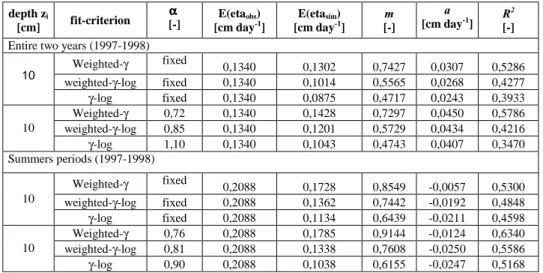
(13) Parameter Estimation Technique. and by R2. Comparison between the case with fixed and varied parameter α, in the Little Washita case. depth zi [cm]. fit-criterion. α [-]. E(etaobs) [cm day-1]. E(etasim) [cm day-1]. m [-]. a [cm day-1]. R2 [-]. 0,1340 0,1340 0,1340 0,1340 0,1340 0,1340. 0,1302 0,1014 0,0875 0,1428 0,1201 0,1043. 0,7427 0,5565 0,4717 0,7297 0,5729 0,4743. 0,0307 0,0268 0,0243 0,0450 0,0434 0,0407. 0,5286 0,4277 0,3933 0,5786 0,4216 0,3470. 0,2088 0,2088 0,2088 0,2088 0,2088 0,2088. 0,1728 0,1362 0,1134 0,1785 0,1338 0,1038. 0,8549 0,7442 0,6439 0,9144 0,7608 0,6155. -0,0057 -0,0192 -0,0211 -0,0124 -0,0250 -0,0247. 0,5300 0,4848 0,4598 0,6340 0,5586 0,5168. Entire two years (1997-1998) Weighted-γ 10. weighted-γ-log γ-log Weighted-γ 10 weighted-γ-log γ-log Summers periods (1997-1998) 10. 10. fixed fixed fixed 0,72 0,85 1,10. Weighted-γ. fixed. weighted-γ-log γ-log Weighted-γ weighted-γ-log γ-log. fixed fixed 0,76 0,81 0,90. It’s interesting to notice the capacity of the technique to evaluate the eta losses using the most superficial p-θ(z1) information. Improved results are observed when etp is estimated from the product of α^ and ETP. The driest periods (the three months during summers) are chosen to test the parametric model on the dry clime, in Little Washita and Duke Forest cases.. Figure 5-3. Simulated vs measured eta in the Duke case, for the entire period (1997-2001) and for the summers of the same period; R2 values for all the three criteria, the weighted-γγ criterion (‘weight’), the weighted-γγ-log criterion (‘w-log’) and the γ-log criterion (‘log’). Parameter α varies..  Hydrology Days 2003. 204.

(14) Toninelli et al.. 6. Conclusions. A new estimation technique of the parameters of a water balance model has been developed, basing on the mass conservation principle and the assumption of stationary conditions. The new technique allows subdividing the total lost outflow in its components, the actual evapotranspiration and the drainage, with good performance in term of the criteria fixed in paragraph 2.1. To do this, the method needs only the precipitation, potential evapotranspiration and the soil moisture data and the model is based on few parameters. Moreover the method works well: (1) when the weighted- γ criterion is used; (2) for different kinds of soil and clime; (3) at point-scale with very good results; at hillslope-scale with good results in dry clime; the actual evapotranspiration is underestimated in wet conditions, probably because the hypothesis of negligible runoff is not respected; (4) considering 1 or few years of data and more years (more information improvs the less good estimations of the actual evapotranspiration); (5) with short times in term of simulation time. It’ll be interesting to add the runoff component of the outflow to see how the complete model applies to every kind of areas. The estimation technique produces good results when applied to measured data and the weighted-γ criterion gives better estimates of the water balance fluxes also in real cases. The estimation method works on data of length shorter than 1 year (Pieve Vergonte case and Little Washita and Duke forest for the summer times) and both in wet than dry conditions. The performances in dry period are better than in wet climatic conditions. When entire year time datasets are considered, the hypothesis of zero runoff is probably not acceptable and it can be the cause of worse results than for summer times. After the application to true measured data is interesting to notice: (1) the most superficial soil moisture seems to estimate the the actual evapotranspiration as well the deeper water content permites; this is a good point for future applications to remotely sensed soil moisture data, that refer to the first centimeters of soil (no more that 10 cm); (2) the results improve using the ‘basic’ ETP; this permits to apply the estimation technique to sites where there are few measured microclimatic quantities for the etp calculation or where the etp estimates are uncertain. The application of the estimation technique to measured data, aggregated at hillslope or regional scale, will be the necessary step to test the model capacity at larger scale. Acknowledgements. This research is part of the MIUR project, "Modellistica idrologica: affidabilità ed assimilazione di dati", through grant #2002074191, and part of CNR-GNDCI project, "Previsione geomorfoclimatica del rischio idrologico", through grant #01.01072.PF42. This research is also part of NASA project, “New scale appropriate diagnostics for evaluating land surface parameterizations and water balance using remotely sensed data”, through grant.  Hydrology Days 2003. 205.

(15) Parameter Estimation Technique. #NAG5-11695. Simunek, J and prof. Katul G. are acknowledged for their. support.. References Ameriflux, http://cdiac.esd.ornl.gov/programs/ameriflux/data2.htm Efron, B., R.J., Tibshirani, 1993: An introduction to the bootstrap, New York, Chapman & Hall. Jackson, T.J., Schmugge, T.J., 1989: Passive microwave remote sensing system for soil moisture: some supporting research, IEEE Trans., Geosci. Remote Sensing, 27, 225-235. Kite, G.W., Droogers, P., 2000: Comparing evapotranspiration estimates from satellites, hydrological models and field data, J. Hydrol., 229, 3-18. Li, J., S., Islam, 2002: Estimation of root zone soil moisture and surface fluxes partitioning using near surface soil moisture measurements, J. Hydrol., 259, 1-14. Meyers, T.P., 2001: A comparison of summertime water and CO2 fluxes over rangeland for well watered and drought conditions, Agric. Forest Meteorol., 106, 205-214. Montaldo, N., V., Toninelli, J. D., Albertson, M., Mancini, P.A., Troch, “Measurements and modeling of actual evapotranspiration for an Italian Alpine catchment”, Hydrology and Earth System Sciences, submitted in October 2002. Mood, A.M., F.A., Graybill, D.C., Boes, 1992: Introduction to the theory of statistics, 1974, McGraw-Hill, Singapore Press, W. H., et alt, Numerical Recipes, Cambridge University Press. National Climatic Data Center, Solar and Meteorological Surface Observation Network (SAMSON), 1990, CD-ROM, http://lwf.ncdc.noaa.gov/oa/about/cdhints.html. Priestley, M.B., 1981: Spectral analysis and time series, Vol. 1-2, London (etc.): Academic Press. Saleem, J.A., G.D., Salvucci, 2002: Comparison of soil wetness indices for inducing functional similarity of hydrologic response across sites in Illinois, J. Hydrometeorol. 3 (1), 80-91. Salvucci, G.D., 2001: Estimating the moisture dependence of root zone water loss using conditionally averaged precipitation, Water. Resour. Res., 37 (5), 1357-1365. Schmugge, T.J., T.J., Jackson, H.L., Mckim, 1980: Survey of methods for soil moisture determination, Water Resour. Res., 16, 961-979. Simunek, J., T., Vogel, M.Th., Van Genuchten, 1994: The SWMS_2D code for simulating water flow and solute transport in two-dimensional variably saturated media, Version 1.2 1. Research Report No. 132, 197, U.S. Salinity Laboratory, USDA, ARS, Riverside, California. Toninelli, V., 1999: L’evapotraspirazione effettiva: confronto tra misure sperimentali e modellistica matematica nei bacini del Toce e del Virginiolo, Thesis for graduation, Milano. Toninelli, V., 2002: Parameter estimation technique for a water balance model and application to measured data, Ph.D. Thesis, Milano..  Hydrology Days 2003. 206.

(16)

No results found