Bayesian Population Viability Analysis for Lynx and Wolverine

(1)

Viability Analysis for

Lynx and Wolverine

in Scandinavia

ISSN 0282-7298

This report presents the results from a demographic population viability analysis, combined with sensitivity analysis, for the lynx (Lynx lynx) and wolverine (Gulo gulo) in Scandinavia under alter-native management scenarios using Bayesian integrated population models. In Sweden, the population growth of both species was sensitive to the individuals’ propensity to disperse to Norway, and also to female survival and recruitment rate. Main drivers of the viability were the choice of harvest strategy, dispersal rates to Norway and the resultant potential for source-sink dynamics, plus the amount of underreported and unknown cryptic poaching.

Rapporten redovisar resultaten från en demografisk sårbarhets-analys, kombinerad med känslighetssårbarhets-analys, av lodjur och järv i Skandinavien under olika förvaltningsscenarier, där Bayesian integrerade populationsmodeller användes. I Sverige påverkas populationstillväxten hos arterna mycket av individernas benägen-het att emigrera från Sverige till Norge, och av honornas överlevnad till vuxen ålder och som vuxna. Huvudfaktorerna för stammarnas livskraft bedöms vara valen av förvaltningsstrategi i de båda länderna, de båda arternas spridning till Norge och den ”source-sink”-dynamik som de kan orsaka, plus mängden illegal jakt.

Rapporta čilge bohtosiid demográfalaš hearkkesvuođa-analysas, ovttas rašesvuođaanlysas, albasiin ja getkkiin Skandinávas sierra hálddahusgovahallamiiguin, gos Bayesian integrerejuvvon populašuvdnašaddan geavahuvvui. Ruoŧas populašuvdnašaddan šlájain sakka váikkuhuvvo indiviiddaid tendeanssas emigreret Ruoŧas Norgii, ja ciikkuid birgen ráves ahkái ja rávvásiin. Váldofáktorat máddagiid eallinfápmui árvvoštallo leahkit hálddahusstrategiija válljen goappaš riikkain, goappaš šlájaid leavvan Norgii ja ”source-sink”– dynamihka man sáhttá dagahit, ja vel man ollu lobihis bivdu lea. Analysis for L ynx and W olverine in Scandinavia Report 6793

Bayesian Population Viability

Analysis for Lynx and Wolverine

in Scandinavia

L. SCOTT MILLS, MARK HEBBLEWHITE AND DANIEL R. EACKER

(2)

SWEDISH ENVIRONMENTAL PROTECTION AGENCY

in Scandinavia

(3)

The Swedish Environmental Protection Agency

Phone: + 46 (0)10-698 10 00, Fax: + 46 (0)10-698 16 00 E-mail: registrator@naturvardsverket.se

Address: Naturvårdsverket, SE-106 48 Stockholm, Sweden Internet: www.naturvardsverket.se

ISBN 978-91-620-6793-9 ISSN 0282-7298 © Naturvårdsverket 2018 Print: Arkitektkopia AB, Bromma 2018

(4)

Preface

This report is written by professor L. Scott Mills (Principal Investigator of the project), professor Mark Hebblewhite (co-PI) and research-associate Daniel R. Eacker (programmer, statistician) at University of Montana (USA). The Swedish summary was written by Per Sjögren-Gulve at the Swedish Environmental Protection Agency (SEPA) and was translated into Northern Sami by Miliana Baer (Vájal Gielain AB). The report has been peer reviewed by Veronica Sahlén (Norwegian Environment Agency), Alexander Winiger (County Administrative Board of Norrbotten, Sweden), and two anonymous reviewers. It presents the results of population viability analyses of lynx and wolverine in Scandinavia and also of sensitivity analyses of the population models.

The SEPA and the report authors thank Per Sjögren-Gulve for coordinating the peer review and production of the report, and for guidance and oversight during development of these PVA models, providing data, and reports, as well as Henrike Hensel, and Peter Jaxgård, from the Wildlife Damage Centre of the Swedish University of Agricultural Sciences for assistance collating lynx harvest data. Comments from expert reviewers greatly helped improve the final version of this report. Photos of lynx and wolverine were reproduced here under the Creative Commons Attribution 3.0 Unported license and the Attribution-NonCommercial-NoDerivs 2.0 Generic, respectively.

The authors assume sole responsibility of the report and its conclusions. The SEPA thanks all who have taken part and contributed in the work. Stockholm, November 2018

Maria Hörnell Willebrand Head of Wildlife Analysis Unit,

(5)

(6)

Sammanfattning

Rapporten redovisar en demografisk sårbarhets- och känslighetsanalys av lodjur och järv i Skandinavien. Naturvårdsverket önskade att analyser genom-förs av effekterna på arternas populationsutveckling och -tillväxt av bland annat olika förvaltningsåtgärder kopplade till jakt i Sverige och Norge, samt effekter av spridning mellan länderna, inavelsdepression samt av täthets-beroende tillväxt. Känslighetsanalysen innebär man med modellsimuleringar undersöker vilka förändringar i individernas överlevnad, reproduktion och/ eller spridning mellan länderna som påverkar populationens eller delbeståndens årliga ökningstakt mest.

Mills, Hebblewhite och Eacker gjorde översikter av publicerade vetenskap-liga artiklar och rapporter, och utformade populationsmodellerna baserat på mer än 30 olika studier. De integrerade data från dokumenterade årliga resultat från skydds- respektive licensjakt i Sverige och Norge från åren 2011–2017, och använde även data från de årliga beräknade beståndsstorlekarna i de två länderna enskilt och tillsammans. Modellernas projektioner gjordes med fokus på de nästkommande 20 åren, vilket motsvarar cirka tre generationer av lodjur och järv demografiskt.

Baserat på de demografiska data för lodjur samt förvaltningen åren 2011– 2017 blev det geometriska medelvärdet av den årliga populationstillväxten (λG)

1,03 i Sverige, dvs. under liknande förvaltning förväntas i genomsnitt en svag populationsökning med ca. 3% per år (konfidensintervall för λG = 0,98–1,08).

I Norge blev λG i genomsnitt 1,01 (med större konfidensintervall, 0,89–1,11).

Givet samma överlevnad, reproduktion och förvaltning, och projicerat framåt, förväntas lodjuret öka något i Sverige med i genomsnitt cirka 5% per år och med cirka 6% per år i Norge. Givet ett modell-scenario med strikt skydd i Sverige förutspådde modellen att lodjuret ökar med i genomsnitt cirka 10% per år i både Sverige och Norge. Med dagens förvaltning indikerar modellens resultat att det är mycket sannolikt att det svenska lodjursbeståndet kommer att vara större än populationsreferensvärdet för gynnsam bevarandestatus (Favourable Reference Population > 870 lodjur) i Sverige under de närmaste 20 åren. Modellen indikerade också att med större beskattning än 10% eller mer än 160 per år i Sverige under samma tidsperiod, ökar risken betydligt för att beståndet blir mindre än 870 lodjur.

I känslighetsanalysen sågs ingen mätbar effekt av inavelsdepression, troligen eftersom det svenska lodjursbeståndet är ganska stort och 20 år (ca. tre lodjursgenerationer) är en kort tidsperiod. Modelleringen indikerade att den gynnsamma bilden ovan starkt kan påverkas av täthetsberoende (resurs-brist) som påverkar vuxna lodjurshonors överlevnad negativt. Resultaten indikerar potentiellt starkt negativa effekter på de skandinaviska lodjurens populationstillväxt av illegal jakt och av s.k. source-sink-dynamik där individer sprider sig till andra områden där dödligheten är betydligt högre, naturligt eller genom jakt. Starkast effekt sågs här av individers spridning från Sverige till Norge.

(9)

I känslighetsanalyserna kopplade till överlevnad, reproduktion och spridning hos de svenska lodjuren (av båda könen), så hade ortstrohet – dvs. att lodjuren inte sprider sig från Sverige till Norge – störst och mycket stark effekt på beståndstillväxten. Därefter var de vuxna lodjurshonornas årliga överlevnad näst viktigast, och därefter överlevnaden av subadulta honor till vuxen ålder samt överlevnaden bland subadulta honor.

För järv blev den genomsnittliga årliga populationstillväxten (λG) 1,01

(konfidensintervall 0,94–1,07) i Sverige och negativ för det norska beståndet (λG = 0,91; intervall 0,83–0,98) under åren 2011–2017. Framåtprojektion under

samma betingelser förutspår i genomsnitt ungefär oförändrad beståndsstorlek i både Sverige och Norge (λG = 1,0). Med strikt skydd i Sverige men inte i Norge,

förutspås en ungefär 3-procentig beståndsökning i genomsnitt per år i båda länderna. Med liknande järvförvaltning som under 2011–2017 under de närmaste 20 åren förutspås en 60-procentig sannolikhet att beståndet i Sverige blir större än 600 järvar. Med strikt skydd i Sverige men oförändrad järvförvaltning i Norge blir den sannolikheten 80 %.

Liksom för lodjur indikerar känslighetsanalyserna att järvens populations-tillväxt påverkas starkt av beskattningen i Norge samt av illegal jakt. Populations-tillväxten påverkas främst av den årliga överlevnaden av unga honor till att bli vuxna, därefter av järvarna ortstrohet (att ej sprida sig från Sverige till Norge) samt av de vuxna honornas årliga överlevnad. Ungdjurens årliga överlevnad, liksom de vuxna hannarnas, hade endast liten påverkan.

Slutsatserna från analyserna är att livskraften (population viability) hos bestånden av lo och järv i Sverige mest påverkas av beskattningen (i båda länderna), spridningen till Norge och ”source-sink”-effekten som den innebär, samt av illegal jakt. Analyserna indikerade inte några betydande effekter av inavelsdepression under de närmaste 20 åren. Det behövs mer kunskap om eventuella effekter av täthetsberoende på populationstillväxten hos båda arterna.

För att uppnå och bibehålla gynnsam bevarandestatus – dvs. ha en bestånds-storlek som minst motsvarar referensvärdet FRP – för arterna i Sverige rekom-menderar författarna att jakt sker endast när beståndet är större än referens-värdet samt är proportionell (% av aktuellt bestånd) eller en bestämd kvot (”fixed quota harvest”). Författarna betonar båda arternas känslighet för illegal jakt och att sådan tillsammans med legal beskattning även i modest omfattning kan få bestånden att minska. Givet den stora effekten på populationstillväxten av spridningen av lodjur liksom järv mellan Sverige och Norge, och vice versa, samt påverkan på den svenska beståndstillväxten av beskattningen i Norge, så rekommenderas fortsatta ansträngningar att integrera och samordna rov-djursförvaltningen länderna emellan och särskilt längs landsgränsen. Då alla simulerings- och modellresultat liksom förvaltningen beror av noggranna populationsberäkningar rekommenderar författarna fortsatt samarbete mellan Norge och Sverige för garanterat samordnad beståndsövervakning, särskilt i ländernas gränsområden.

(10)

Rörande analyserna, så användes s.k. ”Bayesian Integrated Population Models” (IPM) som är stadiebaserade, dvs. individerna i den skandinaviska popula-tionen har för varje art delats upp i grupper efter kön och åldersstadium [t.ex. ungdjur (subadult), reproducerande vuxen, icke-reproducerande vuxen] i res-pektive land samt med överföring (spridande individer) mellan delbestånden i Sverige och Norge. Modellerna konstruerades i open-source-språket R (R Core Team 2016). Även en app baserad på R:s shiny-paket (Chang m.fl. 2017) finns tillgänglig ”open access” på Internet. Den årliga överlevnaden och fort-plantningen av individerna i de olika stadierna och den årliga övergången (andel av individerna) från ett stadium till ett annat, liksom mellanårsvariationen i dessa parametrar, simuleras genom en populations-matrismodell som till-sammans med individerna som finns i de olika stadierna projiceras över de år som simuleras. De årliga överlevnads- och reproduktionstalen i modellen, liksom förflyttningen av individer mellan Sverige och Norge och vice versa, baseras på sammanställda publicerade data. Jakt påverkar överlevnaden hos de stadier som berörs, och i den utsträckning som könsmogna honor fälls så påverkar det även beståndets reproduktion. Beståndens sociala struktur medför att en hane kan fortplanta sig med flera honor under ett år och hannarna antas därför inte begränsa populationens reproduktion. Inavels depression tar sig uttryck som reducerad reproduktion eller minskad överlevnad i den model-lerade populationen på grund av att den är inavlad och individerna är nära släkt med varann, och sänker den årliga populationstillväxten. Likaså kan resursbrist på grund av att det finns så många individer (täthets beroende) påverka den lokala och/eller totala populationstillväxten.

(11)

Čoahkkáigeassu

Rapporta čilge demográfalaš rašes- ja hearkkesvuođaanalysa albasiin ja getkkiin Skandinávias. Luondogáhttendoaimmahat háliidii ahte analysat čađahuvvojedje váikkuhusain šlájaid populašvudnaovdáneamis ja – šaddamis earret iežá sierra hálddahusbijut čadnon bivdui Ruoŧas ja Norggas, ja maid váikkuhusat leavvamiin riikkaid gaskkas, deprešuvdna go lea sagaheapmi ealibiin mat leat ila lahka sogat ja maid valljodatsorjavaš (täthetsberoende) šaddan. Hearkkesvuođaanalysa mearkkaša ahte modeallastimuleremiiguin iskkat makkár rievdadusat indiviiddaid birgemis, laskamis ja/ dahje leavvan riikkaid gaskkas váikkuha populašuvnna dahje oassemáddodaga jahkásaš lassánantávtta eanemusat.

Mills, Hebblewhite ja Eacker ráhkadedje oppalašgeahčastaga almmuhuvvon dieđalaš artihkkaliin ja raporttain, ja hábmejedje populašuvnnamodeallaid vuođđuduvvon eanet go 30 sierra iskamiin. Sii integrerejedje dieđuid dokumenterejuvvon jahkásaš bohtosiin suodje- ja liseansabivdduin Ruoŧas ja Norggas jagiin 2011–2017, ja geavahedje maid dieđuid daid jahkásaš rehkenaston máddodatsturrodagain daid guokte riikkain sierra ja ovttas. Modeallaid projekšuvnnat dahkkojedje deattuin daid boahtte 20 jagiide, mii vástida sullii golbma albbas- ja geatkebuolvva demográfalaččat.

Vuođđuduvvon demográfalaš dieđuid vuođul albasiidda ja maid hálddahus jagiin 2011-2017 geometralaš gaskamearalaš árvu dan jahkásaš populašuvdnašaddadeapmái šattai (λG) 1,03 Ruoŧas, namalassii sullasaš hálddahusas vurdojuvvo gaskamearalaččat

geahnohis populašuvdnalassáneapmi sullii 3% jahkái (konfideansainterválla λG =

0,98–1,08). Norggas šattai λG gaskamearalaččat 1,01 (stuorit konfideansaintervállain,

0,89–1,11). Addon seamma birgema, laskama ja hálddahusa ja projiserejuvvon ovddusguvlui, vurdojuvvo albbas lassánit veaháš Ruoŧas gaskamearalaččat 5% jahkái ja sullii 6% jahkái Norggas. Jus addo modealla-scenario nanu sujiin Ruoŧas einnostedje modeallain ahte albbas lassána gaskamearalaččat sullii 10% jahkásaččat sihke Ruoŧas ja Norggas. Otná hálddahusain modealla boađus indikere ahte lea stuorra vejolašvuohta ahte ruoŧa albbasmáddodat boahtá leat stuorit go populašuvdnarefereansaárvu oiddolaš seailluhanstáhtusii (Favourable Reference Population > 870 lodjur) Ruoŧas daid lagamus 20 jagiid. Modealla indikere maid ahte stuorit vearromáksin go 10% dahje eanet go 160 jahkái Ruoŧas seamma áigodagas, várra lassána sakka ahte máddodat šaddá unnit go 870 albasa.

Hearkkesvuođaanalysas ii oidnon mihtideaddji váikkuhus deprešuvnnas go ila lahka sogat sagahit, jáhkehahtti danne go ruoŧa albbasmáddodat lea oalle stuora ja 20 jagi (sullii golbma albbasbuolvva) lea oanehis áigeáigodat. Modelleren indikerii ahte dat oiddolaš govva bajil garrasit sáhttá váikkuhuvvot valljodatsorjavašvuođas (resursavátni) mii sakka váikkuha ráves albasciikkuid birgema heittot.

Boađus indikere vejolaš garra negatiiva váikkuhusaid daid skandinávalaš albasiid populašuvdnašaddamii lobihis bivddus ja n.g. source-sink-dynamik gos indiviida leavvá iežá guovlluide gos jápmin lea ollu alibut, lunddolaš dahje bivddu bokte. Stuorimus váikkuhus oidnui dás go indiviiddat levvet Ruoŧas Norgii.

Hearkkesvuođaanalysat čadnon birgemii, laskamii ja leavvamii ruoŧa albasiin (goappaš sohkabealit), de báikebissun – namalassii ahte albasat eai leava Ruoŧas Norgii – lea stuorimus ja oalle stuorra váikkuhus máddodatšaddamii. Dan maŋŋil leai ráves

(12)

albasciikkuid jahkásaš birgen nubbin deháleamos, ja dan maŋŋil birgen subadulta ciikkuin ráves ahkái ja maid birgen subadulta ciikkuin.

Geatkái gaskamearalaš jahkásaš populašuvdnašaddan (λG) 1,01 (konfidens interválla

0,94–1,07) Ruoŧas ja negatiiva norgga máddodahkii (λG = 0,91; interválla 0,83–0,98)

jagiid 2011-2017. Einnosteapmi ovddusguvlui oaidná gaskamearalaččat sullii rievdatkeahtes máddodaga sihke Ruoŧas ja Norggas (λG = 1,0). Go lea nanu suodji Ruoŧas muhto i Norggas,

einnostuvvo sullii 3-proseantta máddodatlaskan gaskamearalaččat jahkái goappaš riikkain. Sullasaš geatkehálddahusain dego jagiid 2011–2017 daid lagamus 20 jagiid einnostuvvo 60-proseanta vejolašvuohta ahte máddodat Ruoŧas šaddá eanet go 600 geatkki. Muhto nanu sujiin Ruoŧas ja rievdatkeahtes geatkehálddahus Norggas šaddá jáhkehahtti 80%.

Dego albasiidda hearkkesvuođaanalysa indikere ahte geatkki populašuvdnalaskan váikkuhuvvo sakka vearromáksimis Norggas ja maid lobihis bivddus. Populašuvdnalaskan váikkuhuvvo eanemusat dan jahkásaš birgemis nuorra ciikkuin ja dan maŋŋil geatkki báikebissumii (ahte eai vuolgge Ruoŧas Norgii) ja maid ráves ciikkuid jahkásaš birgen. Nuorra ealibiid jahkásaš birgen, dego ráves rávjjáid, váikkuhii dušše veaháš.

Loahppaboađus analysain lea ahte eallinfápmu (population viability) albasiid ja getkkiid máddodagas eanemus váikkuhuvvo vearromáksimis (goappaš riikkain), leavvan Norgii ja”source-sink”-váiikuhusas maid dat máksá, ja maid lobihis bivddus. Analysat eai indikere makkárge mearkkašahtti váikkuhusaid deprešuvnnas go ila lahka sogat sagahit daid lagamus 20 jagiin. Lea dárbu eanet dieđuide vejolaš váikkuhusain sorjjavašvuhtii galle ealibat leat ovtta guovllus ja populašuvnnašaddamis goappaš šlájain.

Jus galgá ollašuhttit ja doalahit oiddolaš seailluhanstáhtusa – namalassii doallat máddodatsturrodaga mii unnimusat vástida referánsaárvvu FRP – šlájaide Ruoŧas čállit ávžžuhit ahte galgá dušše bivdit go máddodat lea stuorit go refereansaárvu ja lea proporšunála (% áigeguovdilis máddodagas) dahje mearriduvvo eari mielde (”fixed quota harvest”). Čállit deattuhit ahte šlájaid hearkkesvuohta lobihis bivdui ja dakkár bivdu ovttas lágalaš vearromáksimiin oalle unna logut sáhttet dagahit njeaidima máddodagain. Go lea ožžon dan stuorra váikkuhusa populašuvnnašaddamii albasiid ja getkkiid leavvamis Ruoŧa ja Norgga gaskkas, ja nuppos, ja maid váikkuhus dan Ruoŧa máddodahkii go lea vearromáksin Norggas, de ávžžuhuvvo ahte joatkašuhtti rahčamušat integreret ja ovttastahttit meahcceeallehálddáhusa riikkaid gaskal ja erenoamážit riikarájiid mielde. Go visot simuleren- ja modeallabohtosat ja maid hálddahus leat čadnon dárkilis populašuvnnaárvvoštallamiidda ávžžuhit čállit ahte ovttasbargu Norgga ja Ruoŧa gaskkas joatká dáhkidan dihte ovttastuvvon máddodatbearráigeahču, erenoamážit riikkaid rádjeguovlluin.

Mii guoská analysa geavahuvvui ng. ”Bayesian Integrated Population Models” (IPM) mii lea vuođđuduvvon muttuid mielde (stadiebaserad), namalassii indiviiddat dan skandinávalaš populašuvnnas leat juohke šládjii juhkkojuvvon joavkkuide, sohkabeali ja ahkedási mielde [omd.), nuorraealibat (subadult), reproduserejeaddji ráves ealit, ráves ealit mii ii reprodusere] iešguđet riikkain ja maid sirdin (indiviiddat mat levvet) gaskal oassemáddodagas Ruoŧas ja Norggas. Modeallat leat ráhkaduvvon open-source-gillii R (R Core Team 2016). Ja maid App vuođđuduvvon R:s shiny-báhkke (Chang ja earát 2017) lea vejolaš “open access” Interneahtas. Dat jahkásaš birgen ja laskan indiviiddain dain sierra muttuin ja jahkásaš rasten (oassi indiviiddain) ovtta muttus nubbái, dego rievdadusat jagiid gaskkas daid paramehtariin, simulerejuvvo populašuvdna-matrismodeallas mii

(13)

ovttas indiviiddaiguin mat leat daid sierra muttuin projiserejuvvojit dan jagi miehtá mii simulerejuvvo. Dat jahkásaš birgen- ja laskanlogut modeallas, dego sirdimat indiviiddain Ruoŧa ja Norgga gaskkas ja nuppos, leat vuođđuduvvon čohkkehuvvon almmuhuvvon dieđuid vuođul.

Bivdu váikkuha birgema dain muittuin mat váikkuhuvvot, ja nu guhkás go ciikkut mat leat álgán gieibmit goddojuvvot de dat maid váikkuha máddodaga laskama. Máddodagaid sosiála struktuvra mielddisbuktá ahte rávjá sáhttá laskat máŋga ciikkuiguin ovtta jagis ja rávjját eat danne oaivvilduvvot ráddjet populašuvnna laskama. Deprešuvdna go ila lahka sogat sagahit boahtá oidnosii go lea binnun laskan dahje unnun birgen modellerejuvvon populašuvnnas dan siva dihte go indiviiddat leat ila lahka sogat guhte guimmiiguin, ja dáinna vuolidit dan jahkásaš populašuvnnašaddadeami. Maid váilevaš návccat go lea ila ollu indiviiddat

(14)

Summary

This project was motivated by a Swedish Environmental Protection Agency (SEPA) wish to evaluate population viability and effects of management actions on lynx (Lynx lynx) and wolverine (Gulo gulo) in Sweden. Given concerns about potential risk of further decline for these species, and that the lynx declined significantly from 2011 to 2014 and the wolverine from 2012 to 2016, SEPA wanted a demographically-explicit model that could evaluate the effect of management-related actions (including human-caused mortality) on population dynamics and viability. Ultimately, the goal is to contribute to these species being maintained in favorable conservation status in Sweden as required under the European Union (EU) Habitats Directive. Specifically, we were tasked by SEPA to conduct a demographic population viability analysis (PVA), including inbreeding depression, for both lynx and wolverine in the main Scandinavian peninsula with a focus on Sweden.

We developed a flexible Bayesian integrated population model (IPM) to model lynx and wolverine population dynamics using a sex-specific model with 5 stage classes. Bayesian models lend themselves well to conducting population viability analyses (PVAs) as they are flexible, can integrate different data types, account for demographic and environmental stochasticity, and provide results in the form of posterior probabilities of key quantities such as abundance and probability of extinction. We conducted a literature review of published scientific papers and government reports to construct prior distributions for the model, drawing on over 30 studies to obtain parameter estimates for sex- and stage-structured vital rates for Norway and Sweden. We also integrated information from known/reported legal and protective harvest for both lynx and wolverine from the period of 2011–2017 in data-bases provided by SEPA to understand population trends in a retrospective sense immediately prior to 2017. To anchor population projections both retro-spectively and under future scenarios, we used previously published population estimates from the Large Carnivore Initiative for Europe (LCIE) documents for the year 2011. We developed the Bayesian IPM to accommodate different types of harvest, as well as cryptic poaching, potential classic ‘negative’ density-dependence, inbreeding depression, and source-sink dynamics between Norway and Sweden. Our Bayesian IPM was developed in the open-source program-ming language R (R Core Team 2016), and we developed an easy-to-use Application Program Interface (API) based on the shiny package in R (Chang et al. 2017). Our API not only facilitates our modeling for this project, it also allows flexible and user-friendly modeling of other future scenarios.

We then evaluated the consequences of over 40 different management and ecological scenarios on lynx and wolverine population viability. In addition to tracking abundance under different scenarios, we estimated the probability of the population remaining at or above a specified management- relevant abundance threshold (“quasi-persistence probability”). For example, the

(15)

relevant management thresholds we used to track quasi-persistence in Sweden were 870 for lynx and 600 for wolverines, numbers based on previous govern-ment publications. In our API, these thresholds can easily be changed as management objectives are updated. We separately considered the following scenarios from a harvest perspective for both lynx and wolverines: 1) status quo with estimates of harvest from literature studies and harvest databases; 2) complete protection for both species in Sweden; 3) varying levels of a constant proportional harvest; 3) varying levels of a fixed quota system of harvest; and 4) threshold harvest with no harvest below the management threshold and either fixed quota or proportional harvest scenarios above the threshold. We then combined the status quo scenarios with: a) inbreeding depression; b) density-dependence in vital rates; c) source-sink dynamics; and d) cryptic poaching with varying levels of unreported and undetected illegal harvest. We used a Monte Carlo Markov Chain (MCMC) sampling algorithm to simulate posterior distributions of parameters given our input parameters (and variances) for each scenario, and report for each scenario the geometric mean population growth rate, abundance, and probability of exceeding the management thresholds (i.e. quasi-persistence probability) in both Sweden and Norway for the next 20 years.

Focusing first on lynx, during the retrospective time period of 2011–2017, the geometric annual population growth rate, λG, for lynx was 1.03 (95%

Bayesian Confidence Interval, BCI of 0.98–1.08) in Sweden, and lower at 1.01 (95% BCI 0.89–1.11) in Norway, likely because of differential harvest which was higher in Norway. Given status quo vital rates, projecting into the future, Sweden lynx are predicted to experience modest population growth of λG = 1.05 (on average 5% per year; 95% BCI 0.99–1.09) as well as Norway,

1.06 (95% BCI 1.02–1.11). Under the scenario of complete protection, λG

of lynx are projected to increase to 1.10 (1.04–1.14) in both Sweden and Norway (1.10, 95% BCI 1.05–1.14). Abundances of lynx under complete protection and under exponential growth became unrealistically large in 20 years, highlighting the importance of understanding density dependence in vital rates in the future. Under status quo conditions in Sweden, the prob-ability of there being more lynx than the management threshold of 870 was always near 1.0 over all years (2011–2037).

Considering the harvest scenarios, without a threshold below which harvest is set to zero, only the lowest harvest quota of 80–160 lynx or the lowest proportional harvest scenarios of 0.05–0.10 harvest rate led to stationary or increasing population growth and maintained a high and increasing probability of exceeding the management threshold of 870 lynx. For any proportional harvest > 0.10 or quota > 160 lynx in Sweden, λG and abundance decreased,

and probability of falling below the management threshold increased. If harvest is eliminated below the threshold of 870, λG, abundance, and quasi-persistence

probability all stayed stationary or increasing

Next, we report effects of non-harvest factors on population viability of lynx. There were no measurable effects of inbreeding depression on recruitment

(16)

rate under a range of scenarios, because abundances were relatively large and the projection interval (20 years) relatively short. Although empirical evidence is lacking from the field, we next modeled 4 different levels of negative density dependence on adult female survival. Only under no density dependence did the population keep increasing in size, where λG stayed >> 1.0 and probabilities

of quasi-persistence were high.

We found strong effects of source-sink dynamics and cryptic poaching on viability of Sweden’s lynx. The viability of Swedish lynx with a quasi-persistence threshold of 870 was strongly influenced by the different modeled scenarios of dispersal rates to and from Norway/Sweden, but was more influ-enced by increasing dispersal rates from Sweden to Norway. The simulations of increased dispersal from Norway to Sweden had little overall affect on the abundance and quasi-persistence probability for lynx in Norway, but higher immigration from Sweden greatly improved the probability of meeting the management objective for Norway. In the face of even modest levels of addi-tional cryptic poaching (> 0.10 addiaddi-tional harvest rate) in Sweden in addition to status quo levels of harvest, lynx experienced decreased abundance, λG and

probability of quasi-persistence above 870. This emphasizes the key role of understanding cryptic poaching on lynx and wolverine viability in Sweden.

We also conducted a Bayesian-based, life-stage simulation analysis to investigate sensitivity of λG to different vital rates in Sweden. The vital rate

that had the highest impact on λG was fidelity (1 – probability of emigrating

from Sweden to Norway), which had a slope (β) of close to 1 (0.90), and

R2 _{= 0.42 indicating essentially additive effects of emigration from Sweden}

to Norway on Sweden population growth rate. The next 3 most important vital rates were adult female survival (β = 0.69, R2_{= 0.26), the recruitment}

rate for adult female lynx (β = 0.19, R2_{= 0.20), and the survival of subadult}

females (β = 0.24, R2_{= 0.07).}

Next, we summarize results for wolverine. Wolverine λG was stable or

slightly declining between 2011–2017, with λG = 1.01 (95% BCI = 0.94–1.07)

in Sweden, but declining in Norway with λG = 0.91 (95% BCI = 0.83–0.98)

during the same time period. Projecting into the future showed similar growth rates in Sweden of λG = 1.00 (95% BCI = 0.95–1.06) and in Norway with

λG = 1.01 (95%BCI = 0.96–1.02). Under complete protection in Sweden,

but not Norway, λG in Sweden would be expected to increase to 1.03 (95%

BCI = 0.97–1.09), and increase in Norway to 1.03 (95% BCI = 0.97–1.08). Under the status quo management scenario, the probability of exceeding the threshold of 600 wolverines in Sweden was always > 0.60 over the next 20 years, and increases to 0.80 under complete protection in Sweden. Because of the lower threshold, Norway always has a probability of exceeding its thresh-old of ~ 1.0. Similar to the lynx harvest scenarios, without a lower threshthresh-old, only modest amounts of proportional harvest rates (0.03) or a modest quota (18) maintains λG > 1.0 and a high probability of exceeding 600 wolverines.

Again, similarly to lynx, introducing a threshold of no harvest when N < 600 stabilizes population growth rates, size, and persistence probabilities. Also

(17)

similar to lynx, there were no strong effects of inbreeding depression nor realistic effects of density dependence on wolverine population dynamics and persistence.

As with lynx, population viability of wolverine in Sweden was very sensi-tive to harvest in Norway and cryptic poaching. Population growth rate of wolverine in Sweden were most sensitive, in rank order, to: recruitment rate of adult females (β = 0.28, R2_{= 0.43), fidelity (}_{β =0.94, R}2_{=0.31), adult female}

survival (β =0.84, R2_{= 0.27), whereas male and female subadult survival, as}

well as adult male survival had little effect on population growth rate.

In conclusion, we found that the main drivers of the viability of lynx and wolverine in Sweden were the choice of harvest strategy, dispersal rates with neighboring Norway and the resultant potential for source-sink dynamics, and the amount of underreported and unknown cryptic poaching. Given current abundances of lynx and wolverine in Sweden, at approximately 1 650 and 550, there is minimal concern for short-term (20-year) effects of inbreeding depression. And given the dearth of empirical evidence, we do not recommend considering density-dependence in current scenarios. Nonetheless, our results highlight the important need for a better understanding of how vital rates of lynx or wolverine are affected by density in the future given projected positive population growth under, for example, status quo scenarios in Sweden.

In terms of recommendations, the best harvest strategy in Sweden to maintain the minimum threshold abundance seems to be either proportional or a fixed quota harvest that occurs only above this management threshold. We also highlight the sensitivity of Swedish lynx and wolverine population growth to the level of unreported, or cryptic, poaching. Even modest levels of additive cryptic poaching can drive Swedish lynx and wolverine populations to decline under status quo harvest rates. Given the importance of movement between Sweden and Norway to population viability of Swedish lynx and wolverine populations, and the dependence of Swedish population growth rate on Norway harvest scenarios, we recommend continued efforts to integrate carnivore management especially along the long border between Sweden and Norway. Finally, all of our simulations depend on accurate population estimates, especially given this transboundary movement, to inform future manage ment. We recommend continued joint collaboration between Norway and Sweden to ensure that, again, especially in the border regions of both countries, lynx and wolverine population estimates are coordinated.

(18)

1. Background and motivation

of population analyses

This project was motivated by a wish from the Swedish Environmental Protection Agency (SEPA) to evaluate population viability and effects of management actions on lynx (Lynx lynx) and wolverines (Gulo gulo) in Sweden. Given concerns about potential further declines for these species, and that the lynx declined significantly from 2011 to 2014 and the wolverine from 2012 to 2016, SEPA asked for a demographically-explicit model that could evaluate various scenarios in a population viability context, and the role of various management-related actions (including hunter-caused mortality) in affecting population dynamics. Ultimately, the goal was to contribute to these species being maintained in favorable conservation status in Sweden as required by the EU Habitats Directive (92/43/EEG).

Specifically, we were tasked by SEPA to conduct a demographic population viability analysis (PVA), including inbreeding depression and sensitivity analyses, for both lynx and wolverine in the main Scandinavian peninsula with a focus on Sweden, but given the importance of potential immigration/emigration with Norway, to consider Norway as well. In addition to understanding the general population viability under current/historic conditions, we were asked to evaluate the effects of different management scenarios, including different harvest strategies, on the population viability of these two carnivores. Further-more, we were asked to conduct a sensitivity analysis of which demographic, inbreeding, age structure, or other factors have the strongest effect on popu-lation growth rate, risk of decline, as well as highlight data gaps and key parameters for which data were deficient in the scientific literature. Lastly, we were asked to address potential population monitoring strategies, given the implications of our PVA and sensitivity analyses, to SEPA. Our work complements recent PVA analyses conducted for large carnivores in Sweden by other authors (e.g., Nilsson 2013, Puranen-Li et al. 2014, Bruford 2015).

In this report, we describe a Bayesian integrated population model (IPM) that we developed to perform these analyses for wolverines and lynx in Sweden. Our model is developed in the open-source R statistical programming environ-ment (R Core Team 2016). This model features a user-friendly ‘front end’ (e.g., an Application Program Interface or API) that facilitates a sex- and stage-structured demographic PVA (including the potential to incorporate stochasticity, inbreeding depression, density dependence, connectivity with Norway, and harvest). Such a model can be used to evaluate which factors most affect population dynamics and persistence.

Our report contains the following components: a) overview of the popu-lation viability analysis concepts underlying our approach; b) background on the ecological, genetic and management-relevant components included in the model; c) management outcomes and scenarios evaluated in the two species models; d) general methods underlying our modeling framework; e) input

(19)

parameters and results for lynx; f) input parameters and results for wolverine; f) results; g) discussion/conclusions, and h) appendices (Note: source R code for the basic Bayesian IPM for two species is included in appendices). We also provide a revised version of the software to run the program following feedback from the SEPA review.

(20)

2. Overview of population viability

approaches and concepts

1

Here we give a general overview of key concepts related to Population Viability Analysis (PVA) that underlie our approach. PVA can be defined as “the appli-cation of data and models to estimate likelihoods of a population crossing thresholds of viability within various time spans, and to give insights into factors that constitute the biggest threats” (Mills 2013:227).

Although many approaches to quantitative population viability analysis (PVA) exist, two main classes can be distinguished. The first projects time series of population counts. The mean stochastic population trend and its process variance are first calculated from the time series of abundance (or abundance index) estimates. Then, in its simplest form, the trend and variance estimates are used in a random walk or diffusion process to estimate the probability that a population will stochastically decline to a threshold size of concern (quasi-extinction or persistence threshold) in a specified time (e.g,, Dennis et al. 1991, Boyce 1992, Morris and Doak 2002). Viability (or population persistence) is driven by the mean and variance of the stochastic growth rate. If the mean growth rate is large, and the variance in growth rate relatively small, then even quite small populations will be likely to persist far into the future. Conversely, regardless of mean growth rate or abundance, populations with large variance in growth rate will have higher risk of extinction. Typically, mechanistic-based drivers of population dynamics (e.g., inbreeding depression, management actions, anthropogenic stressors) are not easily incorporated in these time series-based approaches, nor do they lend themselves to demographic sensitivity analyses. Another major complication are challenges in obtaining accurate estimates of abundance over time, where survey methods often provide only raw counts, not true population estimates, and field survey methods often change, obscuring the true population process because of substantial sampling variation.

The second major class of PVA models is often called “ demographically explicit” to capture the fact that births, deaths, age structure, stressors, and immigration/emigration can be accounted for. Within this framework, mechanistic factors that affect population dynamics through age-specific vital rates (birth and death rates) can be explicitly modeled. These factors include, for example, density dependence, harvest, and genetic factors such as inbreeding depression. This ability to model inbreeding depression is especially important because for over 20 years it has been known that demo graphic and genetic effects interact to increase vulnerability to extinction in remnant or small populations (Mills and Smouse 1994). That is, in small populations, deterministic stressors (e.g., overharvest, disease, invasive species) decrease

1 _{Parts of this section are adapted from the Final Report to SEPA by the PI on a synthesis of}

(21)

vital rates, that in turn decreases the census and effective abundances, which exacerbates the effects of stochastic fluctuations and inbreeding depression, further decreasing vital rates, and so on. This process is captured by the “extinction vortex” (Figure 1).

These processes interacting in the extinction vortex to alter a population’s probability of persistence (Figure 1) are precisely the dynamics accounted for by demographically explicit PVAs.

For many reasons, PVAs should be interpreted more as an arbiter of the relative effects of different management actions than as a reliable predictor of exact population outcomes. For example, density dependence – including both the specified carrying capacity (K) and the functional form used to describe density dependence (e.g. ceiling, logistic, Allee) can vastly affect the outcomes of PVA predictions, causing different PVA models to have widely divergent predictions even when the input data (e.g. vital rates and their variances, abundances and age structure, etc.) are identical for the different models (Mills et al. 1996).

Figure 1. From Mills 2013, modified from Soulé and Mills (1998). A simplified representation of the extinction vortex. The effects of deterministic stressors are filtered by the population’s environ-ment (habitat as well as variable extrinsic factors such as weather, competition, predators, and food abundance) and by its structure (including age structure, sex ratio, behavior, density dependence, physiological status, and intrinsic birth and death rates). Each turn of the feedback cycle increases extinction probability. The extinction vortex model formalizes the fact that extinction probability arises from an interaction of genetic and nongenetic factors.

(22)

A demographically explicit PVA model also directly accommodates analysis of the relative ‘importance’ of different vital rates and management actions. Broadly speaking, ‘sensitivity analysis’ refers to how changes in vital rates – due to either a natural change or through management – may change popula-tion growth or persistence (Mills and Johnson 2013). Such sensitivity analyses facilitate an assessment of the relative effects of different management actions for meeting population goals. Although matrix-based calculation of analytical ‘elasticities’ and ‘sensitivities’ (based on eigenanalysis of the mean matrix) were an early form of ‘sensitivity analysis’, other approaches currently exist to more realistically accommodate real-world changes to vital rates through management actions (Mills 2013). Here we emphasize sensitivity analyses accomplished through manual perturbation and life-state simulation analysis (LSA).

Manual perturbations simply use the PVA modeling framework to ask “what if” scenarios. For example, if survival changed by 5%, what would the effects be on abundance, viability, etc? This flexible and powerful approach allows the user to perturb vital rate and management possibilities in sensible and transparent ways to assess future growth rate, abundance, or persistence. Different vital rates can be perturbed by any amounts simultaneously, as would occur under real-world management actions.

Life-stage simulation analysis (LSA) standardizes the manual perturbation method to provide insights into the relative effects of various management actions including harvest or other forms of mortality (Wisdom and Mills 1997; Wisdom et al. 2000, Hoekman et al. 2002, Gerber et al. 2004, Johnson et al. 2010a, Taylor et al. 2012). In brief, the LSA approach builds thousands of plausible matrices from the specified means and variances of stage-specific vital rates. Population growth rate (asymptotic or non-asymptotic λ) are calculated for each matrix. Baseline scenarios can be compared to various management alternatives with a variety of metrics (e.g., probability of posi-tive population growth, R2_between_{λ and different vital rates). Eacker et al.}

(2017) recently extended the LSA approach to Bayesian IPMs, showing that Bayesian population analysis could be used to derive analytical sensitivity parameters (i.e., based on eigenvectors and eigenvalues) and generate simu-lated values for LSA within an IPM. Thus, Bayesian IPMs provide a flexible tool to estimate demographic rates, conduct population viability analysis, and understand population dynamics through broad scale sensitivity analyses to provide the most precise information to managers that are tasked with making challenging conservation decisions.

(23)

3. Ecological, genetic and

management-relevant components

included in our models

We used Bayesian methods to forecast Eurasian lynx and wolverine population dynamics in Sweden in a PVA framework that includes sensitivity analyses. The use of Bayesian integrated population models (IPMs) has become more common in assessing population dynamics because of their ability to overcome many of the limitations imposed by traditional analyses (see Schaub and Abadi 2011). In contrast to traditional methods, Bayesian IPMs estimate demographic param-eters in a single, comprehensive, stage-based model to exploit all available information (e.g., harvest, count, capture-mark-recapture data) about popula-tion processes (Johnson et al. 2010b, Schaub and Abadi 2011). The benefits of this approach are that parameter estimates become more precise due to joint estimation, process and sampling mechanisms are specifically accounted for, estimates for years with missing data can be inferred, and covariates (e.g., inbreeding depression, density dependence) can be simultaneously modeled. Bayesian methods are also often easier to implement than classic frequentist approaches. Bayesian IPMs can be customized for population viability analyses to evaluate the probability of a population being below a quasi-persistence threshold of either N or λ (Kéry and Schaub 2012; Bauer et al. 2015). For instance, persistence probabilities are easily derived from the posterior distri-butions of parameters (e.g., Bauer et al. 2015). This allows easy calculation of the probability that a population will be above or below some threshold

N or λ in given year. Further, scenarios evaluating the relative importance of various management actions on population growth (e.g. sensitivity analyses) are easily incorporated.

Next, we briefly describe some of the ecological, genetic, and management-based concepts included in our Bayesian PVA and sensitivity analysis. The specific modeling of these factors are described in Section 4.0, Population Viability Analysis Methods, and the particular values for each model species in Section 5.0 – Lynx and Section 6.0 – Wolverine.

3.1 Stage and Age Structure

Animal population ecologists and managers are often interested in the dynamics of specific age classes or stage classes. First, different stressors and management actions affect different stages of animals in different ways. Second, stage classes and stage-specific vital rates are not equal in their effects on population growth, so that management actions that target different stage classes will not be equal in their effectiveness. Third, different stages may have different values to the public (especially in animals where males of different stages are harvested).

(24)

One useful way to account for age or stage structure is through matrix models (Mills and Smouse 1994, Mills 2013, Caswell 2001). A population matrix model provides a convenient accounting system to track stage- specific vital rates and abundances through time to determine how different vital rates and stages affect dynamics. The sex- and stage-specific model we developed for lynx and wolverine accounts for four stages: a) subadults (or yearlings) of both sexes; b) 2-year old females; c) adult females; and d) adult males, with accompanying vital rates. These stages are projected through a 4 × 4 matrix model (see section 5.2 below).

Importantly, the fact that different stage classes will differentially affect population growth means that the number of animals in each stage class can have substantial effects on population growth. Under constant conditions any initial stage distribution will converge on an asymptotic stable stage distribu-tion (SSD) and asymptotic growth rate (λSSD) characteristic to the particular

vital rates in the matrix (Mills 2013, Caswell 2001). However, if the initial stage distribution is not in SSD then transient dynamics (or population inertia) will occur that will cause population growth to be greater or less than λSSD

depending on the reproductive values of the stages in the initial population vector (Caswell 2001, Koons et al. 2006). Practically speaking, this means that a deterministic population projection initiated with 100 animals and an expected asymptotic growth rate at SSD of 10% per year ( = 1.1) would have 110 animals after 1 year if the initial population is distributed at SSD, but could have much fewer (perhaps 95) or much more (perhaps 115) if the initial stage distribution is far from SSD (see examples in Mills 2013, Chapter 6).

Despite the importance of initial age distribution, there is little known about age distribution of large carnivores such as lynx and wolverine in Sweden. Therefore, we used the default of distributing the initial distribution of initial abundances for both species in our model according to the SSD given our vital rates. However, we also allow the user interface of our model for user input of any alternative initial stage distribution. In the case of starting at SSD, the population will grow asymptotically without any fluctuations due to transient dynamics in stage distribution (Mills 2013, Caswell 2001). If the user enters any other initial stage distribution, they should know that population growth will – for several years – be more or less than λSSD purely due to transient

dynamics until asymptotic convergence to SSD. Also, variation in retrospective harvest rates will cause population growth rates to bounce around initially, but the population will return to constant growth once harvest is kept constant. Finally, we did not explicitly account for senescence by truncating fecundity or survival above some fixed age, or according to some function (Caswell 2001), in part because of the lack of empirical evidence for senescence in large carnivores such as lynx and wolverine.

(25)

3.2 Stochasticity

Two main forms of stochasticity, or variation, affecting vital rates can be dis-tinguished that should be included in any population projection model. First

demographic stochasticity arises from random deviations that arise in a

deter-ministic (non-varying) environment simply because whole animals experience probabilistic, often binomially distributed (0, 1) vital rates (e.g. an animal with a 70% survival cannot 70% survive; either it lives with 70% probability or dies with 30% probability). Demographic stochasticity is analogous to coin-flipping (i.e., Bernoulli) variation around an expected mean of 50:50, where the expectation is driven by the vital rate mean. The effect of demo-graphic stochasticity disappears as abundance exceeds about 100 and the expected mean converges on the actual mean (Morris and Doak 2002).

While demographic stochasticity occurs even in totally deterministic, constant conditions, environmental stochasticity incorporates variability in the mean vital rate over time as environmental conditions change. Weather often drives environmental stochasticity (e.g. wet versus dry years), as do unpredictable disease outbreaks or changes in predator abundance. Notably, environmental stochasticity affects growth rates at any size of population (unlike demographic stochasticity). As an aside, we note that ‘genetic sto-chasticity’ – the random variation in allele frequencies (and associated fitness costs of inbreeding) at small populations is described below in a section on “Inbreeding Depression”.

3.3 Density Dependence

Density dependence arises when a population’s density or abundance affects the vital rates of individuals in the population, which in turn can affect the population growth rate. Classic, or negative density-dependence occurs when factors such as parasitism, predation, or intraspecific competition for resources lead to a reduction in vital rates as populations increase in size. Negative density dependence tends to be regulatory, as it reduces population growth at high abundance and increases it at low abundance. This regulation leads to stable fluctuations around a long-term mean abundance where popu-lation growth rate is stationary at carrying capacity (K) (Mills 2013). At K, births = deaths, and the population stabilizes, dependent on the degree of environmental stochasticity. Although the simplest and most common way of modeling negative density dependence is the logistic (or discrete-time form, the Ricker), this assumes that all density dependence is negative, in a linear fashion from 0 to carrying capacity, and that the carrying capacity can be quantified from field data. Another form of pseudo density dependence is the ‘ceiling model’, whereby population growth is exponential to K, but can never increase above K. A ceiling type model is unrealistic for most species, with possible exceptions being those with very strong territoriality or a strict limiting resource such as nest boxes or overwinter spots.

(26)

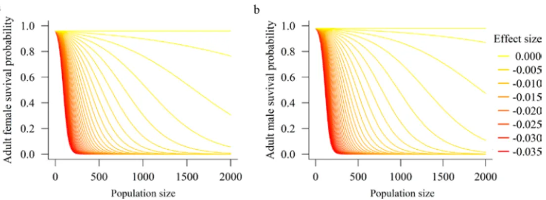
To our knowledge, none of these assumptions can be evaluated based on field studies of density-dependence in wolverines and lynx. Only 1 study in the literature reports evidence for density-dependence in a single vital rate, adult survival, for wolverine in one study area in southern Sweden (Brøseth et al. 2010). While this provided some evidence for density-dependence in a single vital rate, it has not been demonstrated that this translated to density dependence in population growth rate around a carrying capacity. There might be compensation amongst vital rates as adult survival declined at higher densities, for example, with increased recruitment or fecundity. And for lynx, there were no studies demonstrating density-dependence anywhere in Scandinavia. One difficulty in applying the results of Brøseth et al. (2010) is that the abundances from which density dependence estimates were derived ranged from 70–120, far lower than the population sizes of wolverine or lynx in either Sweden or Norway that were modeled in the PVA. Despite this considerable uncertainty in how density dependence would operate at these larger spatial scales and population sizes, and without any evidence for lynx, we included it in our PVA using the same form as found by Brøseth et al. 2010, whereby adult survival declined as density increased. Therefore, our default scenarios did not include density-dependence but we evaluated sensi-tivity of results to differing strength of density-dependence in PVA analyses for both wolverine and lynx.

In addition to negative density dependence, at small population sizes, wild populations might experience “Allee effects” or positive density dependence, whereby vital rates correlate positively with density, especially at low densi-ties (Mills 2013). Mechanisms driving positive density dependence include cooperative defense, foraging efficiency, mate finding, and rearing of offspring (Kramer et al. 2009, Gregory et al. 2010). When these mechanisms occur, a decreasing abundance leads to decreased vital rates and population growth rate. We found no scientific literature on which to parameterize positive density dependence for our focal species; therefore, the current model contains no positive density dependence. (Parenthetically, some would consider inbreeding depression to be a form of positive density dependence, as vital rates are decremented as abundance declines; we do include inbreeding depression in our model [see next section]).

3.4 Inbreeding Depression

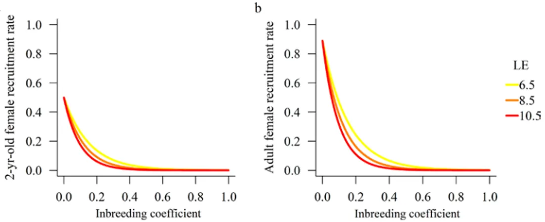
Inbreeding depression arises in cases when a loss of heterozygosity due to inbreeding translates into a decrease in one or more vital rates (e.g. survival, reproduction, Allendorf et al. 2013, Mills 2013). In essence, inbreeding can occur through two mechanisms: a) preferential non-random mating with relatives (denoted by F_is); and b) genetic drift arising from random mating in small populations (denoted by F_st). Inbreeding via preferential mating can usually be dismissed in most wild vertebrates, so that ‘inbreeding’ (F) in small populations of conservation concern arises from genetic drift (e.g. F= F_st).

(27)

This form of inbreeding quantifies the loss of heterozygosity based on the genetic effective population size (N_e) over time (See Box 1). Juvenile survival is often considered to be the vital rate most affected by inbreeding, because inbreeding depression in this stage would purge deleterious alleles from being expressed in later stages. However, arguments have been made for including inbreeding depression in other vital rates, which would increase the overall effect of inbreeding depression on population dynamics (Allendorf et al. 2013, O’Grady et al. 2006).

Although inbreeding depression can absolutely drive population declines and increased extinction risk, it should not be considered axiomatic that inbreeding depression will always have these negative population-level effects. For example, Johnson et al. (2011) show that endangered Sierra Nevada big-horn sheep suffered statistically significant inbreeding depression on fecundity. However, incorporating these costs of inbreeding into a matrix projection model showed that the inbreeding depression on sheep fecundity would have minimal effect on short-term population growth, implying that other manage-ment actions would be more effective at short-term recovery than would genetic rescue to address inbreeding depression. In general, inclusion of inbreeding depression in a PVA is appropriate to evaluate its potential effect on viability.

PVA models often account for inbreeding depression by decrementing vital rates based on inbreeding coefficient (due to drift) at that time step and the specified cost of inbreeding. The ‘inbreeding load’ (or ‘lethal equivalents per gamete’), commonly denoted as B, can be calculated empirically as the rate at which survival (or other fitness attributes) declines with increased inbreeding (Morton et al. 1956, Hedrick and Kalinowski 2000). Because species-specific estimates of inbreeding depression are often lacking for species of conservation concern, PVA models often evaluate ‘what if’ scenarios based on reasonable ranges of inbreeding depression derived from the literature. In the most classic paper quantifying lethal equivalents, Ralls et al. (1988) estimated 1.57 lethal equivalents per gamete (= 3.57/diploid genome) as the median B for juvenile survival in 40 non-domestic mammal species in cap-tivity. This median value is the default value for incorporating inbreeding depression in the PVA Program “VORTEX” (Lacy and Pollak 2014). Sub-sequent reviews have generally supported B = 1.57 as a reasonable rule of thumb for inbreeding load on juvenile survival (Keller and Waller 2002, Crnokrak and Roff 1999). However, these reviews and others (e.g., Fox and Reed 2010) have noted that the captive conditions of Ralls et al. (1988) may have biased low estimates of inbreeding because the higher stress conditions in the wild substantially increases the cost of inbreeding compared to the more benign captive conditions. For these reasons, in a PVA for Scandinavian wolves, Nilsson (2013) used higher lethal equivalents (B from 6.5–10.5) and found strong effects of inbreeding on the viability of the relatively small Scandinavian wolf (Canis lupus) population.

Gven a specified cost of inbreeding (B), the proportionate reduction in fitness at a particular inbreeding coefficient (F) is: G = 1–e(-BF)_{(Morton et al.}

1956, Keller and Waller 2002; See FOOTNOTE 2 BELOW). Therefore, in a matrix model the non-inbred survival rate (S ) for a given cohort in a given

(28)

time step is decremented by the cost of inbreeding to give the survival under inbreeding (S_F) as (Mills and Smouse 1994)2_{: S}

F = S0 * (e (–BF)).

For our lynx and wolverine PVA models, we set F=0 for the beginning of each simulation. The model then increments F at time step t by the classic for-mula based on effective population size (Ne): F(t) = 1–(1–1/[2 N_e])t_{~ 1–e}-t/[2Ne]_.

The genetic effective size (Ne) is the size of an ideal population that would lose heterozygosity due to genetic drift at the same rate as the actual popula-tion in quespopula-tion; thus, Ne provides a standardized baseline to estimate the expected loss of genetic variation due to genetic drift. Practically speaking, Ne is always smaller than the population head count, or census size (N). How much smaller Ne is than N varies widely according to mating system and life history. For monogamous or mildly polygynous mammals, ratios of Ne/N tend to be in the range of 0.3 to 0.5. There are few published estimates for Ne/N ratios for Eurasian lynx and wolverines, so we used a range of ratios of 0.3 to 0.5.

For the wolverine and lynx models, empirical estimates of the cost of inbreeding (B) do not exist. In the absence of any estimates of inbreeding depression for any wild lynx or wolverines, we used a range of values of

B = 6.5–10.5 following from the Nillson (2013) PVA and imposed the effect

on recruitment rate. This was equivalent to imposing an effect on juvenile survival since recruitment rate (the number of offspring surviving to age 1 per breeding adult female) is the product of juvenile survival, litter size, and proportion of females that breed. Although these values of B are at the upper end of estimated values (see reviews above), we are not modeling inbreeding depression on other vital rates such as subadult or adult survival. Further iterations of this model could easily incorporate inbreeding depression on other vital rates.

3.5 Human-caused Mortality

Relevant deterministic stressors are an essential component of PVA models. Although stressors often include habitat loss, predation, disease, and climate change, for the target species evaluated here the biggest perceived stressor is human-caused mortality (Kaczensky et al. 2012, Chapron et al. 2015). This may include legal harvest, management removals, or poaching. Harvest can be considered along a spectrum from completely additive mortality, where every removal subtracts from total abundance, or completely compensatory, where every removal is replaced without a decline in abundance by a new recruit (Mills 2013). This represents the scenario where mortality from one source (e.g., harvest) offsets mortality from other sources (e.g., starvation).

2 _{Note: This formulation assumes multiplicative fitness costs across loci; Mills and Smouse (1994)}

note the strong evidence for synergistic formulations that yield nonlinear results for higher values of F. Simply put, this can be modeled by replacing F with [G= F/(1-F)]; we use this approach for this model, a somewhat conservative approach as F remained small for the relatively large Ne of wolverine and lynx.

(29)

In reality, the degree to which harvest falls on this continuous spectrum from completely additive to completely density dependence varies on species life-history, density-dependence (i.e., most harvest tends to be compensatory at higher densities approaching carrying capacity), and other factors such as weather.

For large carnivores, in general, there is conflicting evidence for strong compensatory mortality, and more evidence in general that harvest by humans tends to be additive (but see Murray et al. 2010). Nevertheless, in the case of our two-focal species, lynx and wolverine, there was little direct evidence for human-caused mortality being additive or compensatory. Thus, we adopted the approach of modeling a range of additive harvest rates from zero to very high levels, that could conceptually represent varying degrees of compensatory harvest. For example, if we modeled a total additive harvest of 0.10, this could be considered equivalent to a partially compensatory harvest rate of 0.20 if managers felt that indeed, compensatory mortality was justified for lynx and wolverine.

Two general classes of harvest strategies include a fixed quota harvest (removing a fixed number of individuals each time step), and fixed-effort harvesting (where a constant proportion is harvested so that fewer individuals are harvested when the population is small) (Lande et al. 1997, Saether et al. 2010, Mills 2013). Often, wildlife managers use a combination of methods combined with a threshold denoting break points of different management strategies; for species of concern, there may be no harvest below the threshold. Finally, there can be cryptic poaching where some additional amount of har-vest is illegal, undetected, or unreported (Liberg et al. 2012). Usually, the only way to estimate such cryptic poaching is via tracking of marked animals, for example, through radiotelemetry. As an example, McLellan et al. (1999) showed that reported harvest of grizzly bears (Ursus arctos) from legal harvest underestimated total mortality (which included poaching) by 50%. However, recent studies suggest that cryptic poaching may be still underestimated even when using radiotelemetry (Liberg et al. 2012). Similar to other effects on vital rates, harvest or cryptic poaching can be incorporated as a deterministic parameter in PVA models. For example, a fixed-harvest rate can be set that reduces abundance at the next time step, or, harvest can be integrated directly from field estimates that already account for harvest mortlaity. In addition, ‘extra’ cryptic poaching can also be deterministically added. And in the con-text of Bayesian PVA, these deterministic harvest rates are then incorporated into stochastic simulations of vital rates and abundance to explore consequences to population viability.

3.6 Connectivity Among Multiple Population

The framework of single-population PVAs can be extended (if sufficient input data exists) to multiple populations. The general principles to emerge from theory and practice with multiple population PVAs is that persistence of both

(30)

individual populations and the greater metapopulation are highly affected by connectivity (both demographic migration and gene flow) and by the degree of correlation in population dynamics among the individual populations. In the context of understanding population viability of the main Sweden popu-lations of lynx and wolverine, it is important to understand the potential impacts of potential source-sink dynamics between Sweden and adjacent Norway. These two countries share a long, permeable border, and there is abundant evidence of movements, immigration and emigration across this border by Scandinavian carnivore populations including bears (Bischof et al. 2015), wolves (Kojola et al. 2009), lynx (Linnell et al. 2001), and wolverine (Gervasi et al. 2015). Here, we considered basic source-sink dynamics between populations of lynx and wolverine in Sweden and Norway, respectively, based on a previous studies that measured dispersal in wolverine (Gervasi et al. 2015). We considered that all non-juvenile age classes could migrate between adjacent countries, and provide more species-specific details below in Section 5.0 and 6.0. In general, harvest-related mortality was higher for both lynx and wolverines in Norway compared to Sweden. We considered a variety of differential harvest scenarios to help inform the consequences of harvest in Norway to the viability of lynx and wolverine in Sweden.

3.7 Outputs of PVA: projection intervals,

quasi-extinction thresholds, and

probability distributions

PVA outcomes are fundamentally defined by the projection interval, or time span over which projections are made (Frankel and Soulé 1981). As with any other prediction (e.g., weather, stock market), the assumptions (and therefore predictions) of PVA will be less and less reliable further into the future. Scott et al. (1995) proposed that when PVA is used in endangered species recovery plans it should incorporate short-term projections that are evaluated over time against a long-term goal (see also Goodman 2002). The long-term viability assessment should include goals that are biologically based (but not be so far in the future as to be patently disconnected from management reality; we would venture that it would be hard to defend >100 years, for example). The short-term projections should explicitly incorporate political/legal/social constraints; monitoring and the iterative application of short-term PVAs can be used to evaluate how well long-term goals are being achieved. Thus, public review (and political trade-offs) can be incorporated in choosing short-term manage-ment strategies, but ultimate success is judged against the yardstick of the long-term, biologically-based goal. Although we use some arbitrary projection intervals in this report (e.g. 20 years), we encourage stakeholders in Sweden to apply these guidelines to develop short and long-term projection intervals.

A variety of metrics may be used in PVA projections. Early PVAs focused strongly on probability of persistence only in terms of avoiding extinction