Ethernet Networks (HS-IDA-EA-97-101)
Thorvaldur Örn Arnarson (valdi@ida.his.se) Department of Computer Science
University of Skövde, Box 408 S-54128 Skövde, SWEDEN
Final Year Project in Computer Science, spring 1997. Supervisor: Jörgen Hansson
Submitted by Thorvaldur Örn Arnarson to Högskolan Skövde as a dissertation for the degree of BSc, in the Department of Computer Science.
13. June 1997
I certify that all material in this dissertation which is not my own work has been identified and that no material is included for which a degree has previously been conferred on me.
Thorvaldur Örn Arnarson (valdi@ida.his.se)
Key words: data communication, switching technology, network design, Ethernet,
Fast Ethernet.
Abstract
Today’s broadcast based shared media networks are beginning to be the bottleneck of computer systems in many organizations. A new networking paradigm, frame and cell switching, promises to meet the ever-increasing demands for network services. The objective of this project is to create design guidelines for designing switched network. The restriction was made to only focus on layer 2 switching in IEEE 802.3 (Ethernet) and IEEE 802.3u (Fast Ethernet) networks.
Performing benchmark tests on a few different network architectures, and then comparing the results, helped forming the guidelines. In our benchmark test we had nine clients and one server. The only computer the clients communicated with was the server, where clients did not communicate with each other.
The results showed that there was no benefit of using a switch as long as the server was connected to the switch at 10 Mbps. The results also showed that using switches in a wrong way could have negative effect on the throughput of the network. As expected when the switch was used in the right way, the throughput increased significantly.
Sammanfattning...1
1
Introduction ...2
1.1 Report Outline ... 2
2
Background ...3
2.1 Traditional Building Blocks ... 3
2.1.1 Repeater ... 3 2.1.2 Bridge ... 4 2.1.3 Router ... 5 2.2 IEEE 802.3 (Ethernet) ... 5 2.2.1 Transmission Media... 5 2.2.2 Frame Format... 7 2.2.3 Operation of IEEE 802.3 ... 7 2.2.4 Example of a Collision ... 9
2.3 IEEE 802.3u (Fast Ethernet) ... 11
2.3.1 100BaseT4 ... 12
2.3.2 100BaseTX ... 13
2.3.3 100BaseFX ... 13
3
Problem Description...14
3.1 Changing Requirements ... 14
3.1.1 The Move to Server Centralization... 14
3.1.2 Universal IT Trends ... 15
3.1.3 Old Solutions ... 16
3.1.4 The Effect on the Networks ... 17
3.2 Switching – a new Networking Paradigm ... 18
3.2.1 Frame Switching... 18
3.3 Designing Switched Networks ... 19
4
Testing Methodology ...20
4.1 Architectures ... 20
4.1.1 Shared 10 Mbps ... 20
4.1.2 All Clients on one Port of a Switch and the Server on another Port ... 20
4.1.3 3 Clients on 3 Ports and Server on one Port ... 21
4.1.4 All Clients on separate Ports and Server on one Port ... 21
4.3.1 Detailed Description ... 22
4.4 Simulation Settings... 23
5
Analysis...25
5.1 Shared 10 Mbps... 25
5.2 All Clients on one Port of the Switch and the Server on Another... 26
5.3 3 Clients on 3 Ports and the Server on one Port ... 27
5.4 All Clients on Separate Ports... 28
5.5 Summary ... 29
5.6 Correctness of the Test ... 31
5.7 Design Guidelines ... 33
6
Conclusion ...34
6.1 Future Work ... 34Acknowledgements ...36
References...37
Appendix A...38
Appendix B ...42
Dagens nätverk, som är baserade på delat transmissionsmedia samt "broadcast" teknik, tenderar att utgöra en begränsade faktor i organisationers kommunikationsflöden och informationstrukturer. Nya nätverksteknologier, där ibland paket- och cellväxling, ser ut att möta de ökade kraven som organisationer ställer på sina nätverkstjänster med avseende på tillgänglighet, pålitlighet och prestanda. Målet med detta projekt är att ta fram riktlinjer för hur man designar växlade nätverk. Rapportens primära fokus ligger på att prestandaoptimera växling, som utföres på MAC-nivå, i nätverk som är baserade på IEEE 802.3 (Ethernet) och IEEE 802.3u (Fast Ethernet) standarderna.
Till grund för framtagande av riktlinjerna, beskrivs omfattande prestandamätningar på fyra olika nätverksarkitekturer, där nätverksbelastning och trafikstrukturen varierades. Tester utfördes med nio klienter och en server, där klienterna kommunicerade med servern, dvs en asymmetrisk trafikstruktur.
Resultaten påvisar att ett felaktigt designat och växlat nätverk resulterar i en betydande prestandaförlust, som i vissa fall är betydligt sämre än ett icke-växlat nätverk. Korrekt växling resulterade, som förväntat, en signifikant förbättring jämfört med icke-växlade nätverk. Optimal prestanda erhålles då samtliga klienter har en egen port i växeln och servern har en egen höghastighetsförbindelse till växeln. Resultaten visar att god prestanda erhålles om klienter grupperas på växelns portar, vilket innebär en bättre kostnadseffektivitet.
1
Introduction
Today’s computer networks have firmly established themselves throughout information-intensive organizations as strategic business assets that increase efficiency, productivity, and effectiveness. From manufacturing to financial services, transportation to technology, education to government and beyond, these networks produce business benefits by providing critical decisions makers and content providers with instant and easy access to information.
Today’s broadcast based shared media networks are beginning to be the bottleneck of computer systems in many organizations. This is due to several factors. The migration from mainframes to client/server architectures and after that to centralized client/server architectures has had a tremendous effect on the networks. The traffic pattern that the networks were built for has been totally changed.
The popularity of Internet has also had much impact on the network. With the easy-to-use interface of WWW browsers every non-technical person can start surfing the Internet without any training. This has led to the implementation of intranets with the aid of WWW browsers. Through WWW browsers users can jump between servers with a simple click on the mouse button, therefore making the traffic pattern very difficult to predict.
Networks are now at a crossroad. In many organizations the networks are already stressed to their limits and if not they will be in the near future. A new networking paradigm, high-speed frame and cell switching, promises to meet the ever-increasing demands for network services. Using switches when designing networks requires much more planning than with the traditional shared networks. The purpose of this project is to create guidlines for designing switched networks and answer questions such as what will be gained by using switches and what has to be changed in current ways of working. To answer these questions we will do a benchmark test on a few different network architectures. In our tests we will measure the throughput of a network in a client/server architecture where the traffic stream is from the server to the clients.
Switching products are available for Ethernet, Fast Ethernet, Token Ring, FDDI, and ATM technologies. Due to the popularity of Ethernet we will only focus on switching in Ethernet and Fast Ethernet networks.
1.1
Report Outline
The remainder of the report will be organized in the following manner. In chapter 2 we give a background information necessary for this project. Here we will cover the IEEE 802.3 (Ethernet) and Fast Ethernet standards amongst with an introduction of traditional building blocks of network design. Chapter 3 contains a more detailed description of the problem of designing switched networks. In chapter 4 we describe our testing methodology, i.e., what network architectures will be tested and how the test is performed. Chapter 5 contains the results of the benchmark tests and finally chapter 6 contains the conclusion of the project.
2
Background
This chapter contains necessary background information for this project. As the switch is a new device in networking, we begin in section 2.1 by briefly describing the functionality of three traditional building blocks of networking to be able to see the benefits of the switch. Then in 2.2 and 2.3 we describe the IEEE 802.3 (Ethernet) standard and Fast Ethernet standard, respectively, as these are the technologies that this dissertation focuses on.
2.1
Traditional Building Blocks
Here we describe the functionality of three traditional building blocks of network design: repeater, bridge, and router.
2.1.1 Repeater
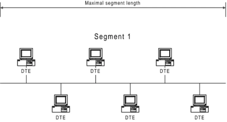
Most medium access control methods have some restrictions on maximal segment length with each type of medium they support. Consider IEEE 802.3 (Ethernet), where the maximal segment length is 500 meters with thick coaxial cable [Tan96]. These restrictions of maximal segment length are due to the attenuation of the signals travelling on the media. This maximal segment length is, however, not always adequate when the network is spread over large area. A repeater is a device that offers the capability to extend an existing segment [Spo96]. Its only functionality is to receive, amplify and forward digital signals. Repeaters use only the physical layer of the OSIRM1, i.e. the lowest layer.
S e g m e n t 1 D T E D T E D T E D T E D T E D T E
Maximal segment length
Figure 2.1 Segment that has reached its maximal segment length.
S e g m e n t 2 Repeater S e g m e n t 1 D T E D T E D T E D T E D T E D T E D T E D T E D T E
Figure 2.2 Segment that has been extended with a repeater.
1 The Open System Interconnect Reference Model outlines a layered approach to data transmission. It
has seven layers with each successively higher layer providing a value-added service to the layer below it [Spo96].
Figure 2.1 shows a segment that needs to be extended, but has already reached its maximal segment length limit. Figure 2.2 shows the segment as it has been extended with the aid of a repeater. Every frame received from segment 1 is amplified and forwarded to segment 2 and the other way around. This means that, in terms of bandwidth, the network behaves like a single segment. The repeater is completely transparent to all DTEs 2on the segment.
2.1.2 Bridge
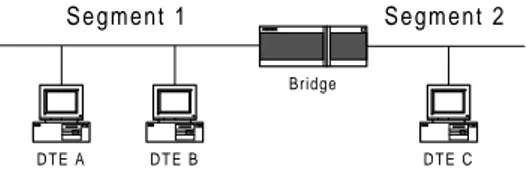
A bridge is a networking device used to interconnect LAN3 and WAN4 segments [Spo96]. The connection can be LAN to LAN, LAN to WAN, and WAN to WAN. Bridges operate at the media access control (MAC) layer of the OSI data link layer (layer 2). The bridge is a store-and-forward device, i.e., different from repeaters which forward every bit as they arrive, bridges receive a frame in its entirety before forwarding it. This means that all frames that the bridge receives from a segment are stored before they are forwarded. Because of this functionality, every frame can be error checked. Bridges only forward frames that are free of errors.
Another key capability of bridges is their ability to filter data. Because the bridge stores each frame it receives, it can read the destination address of each frame and determine whether to forward it or not. Only frames that are addressed to DTEs on a different segment from which it was received are forwarded. Figure 2.3 gives an example of this. Consider that the bridge receives a frame from segment 1 with the destination address of DTE B. Because DTE B is on segment 1 the bridge does not forward the frame to segment 2, however, if the destination address would be DTE C the bridge would forward the frame.
S e g m e n t 2
Bridge
S e g m e n t 1
D T E B
D T E A D T E C
Figure 2.3 Bridged network.
There are four major types of bridges: transparent, translating, encapsulating, and source routing bridges [Spo96]. The two most widely adopted types are transparent and source routing bridges. The main difference between them is the routing algorithm. With transparent bridges, the bridges make all the routing decisions, i.e., the routing is transparent to the DTEs, while with source routing bridges the DTEs perform the routing. A further description of these different types of bridges is outside the scope of this project.
2 DTE, or Data Terminal Equipment is a generic name for any user device connected to a data network
[Hal96].
3 Local Area Network. A network used to interconnect a community of digital devices distributed over
a localized area [Hal96].
4
2.1.3 Router
A router is a networking device used to interconnect two or more LANs and/or WANs together [Spo96]. It provides connectivity between like and unlike devices. Routers operate at the network layer of the OSIRM (layer 3). Routers understand the network and route packets based on many factors to select the best path between any two devices. Examples of such factors are: number of router hops, available bandwidth, delay and utilization.
One of the advantages routers have over bridges is the possibility to control the traffic flow in the network. It is possible to set access lists for each interface on the router stating what DTEs can communicate with the DTEs connected to that interface. Consider Figure 2.3 again. With the aid of access lists it is possible to configure the router so that the only DTE that can communicate with DTE C is DTE A. When DTE B tries to communicate with DTE C the packet is not forwarded to DTE C.
Due to the additional functionality of routers it takes the router longer time to process the frames and decide whether or where to forward the frames.
2.2
IEEE 802.3 (Ethernet)
IEEE 802.3 is an international standard for CSMA/CD (Carrier Sense Multiple Access with Collision Detection) local area networks. Work on the predecessor of IEEE 802.3, Ethernet, began at the Xerox Palo Alto Research center in 1972. Eight years later, in 1980, the first formal specifications for Ethernet (Version I) were published by a consortium of companies consisting of DEC, Intel, and Xerox (DIX). In the same year, the IEEE meetings on Ethernet began. The IEEE standard was first published in 1985, with the formal title of “IEEE 802.3 Carrier Sense Multiple Access with Collision Detection (CSMA/CD) Access Method and Physical Layer Specifications.” The standard has since been adopted by the International Organization for Standardization (ISO), which makes it a worldwide networking standard. The IEEE 802.3 standard is periodically updated to include new technology. Since 1985 the standard has grown to include new media systems for 10 Mbps Ethernet (e.g. twisted-pair media), as well as the latest set of specifications for 100-Mbps Fast Ethernet.
The rest of this section gives a detailed description of the IEEE 802.3 standard.
2.2.1 Transmission Media
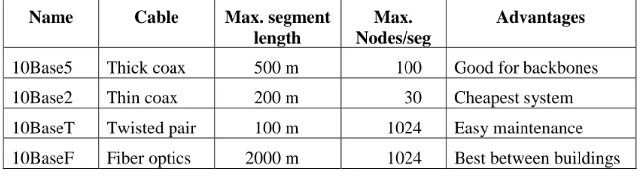
There are commonly four types of cabling used with IEEE 802.3 (see Table 2.1) [Tan96]. Although different media are used, they all operate using the same medium access control method (see section 2.2.3).
Name Cable Max. segment
length
Max. Nodes/seg
Advantages
10Base5 Thick coax 500 m 100 Good for backbones
10Base2 Thin coax 200 m 30 Cheapest system
10BaseT Twisted pair 100 m 1024 Easy maintenance
10BaseF Fiber optics 2000 m 1024 Best between buildings
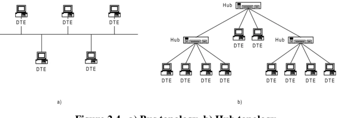
Apart from the cable itself, the main difference between these types of cabling is the topology in which they are used. Both 10Base5 and 10Base2 are used in a bus topology (see Figure 2.4a). With a bus topology a single network cable is routed through the locations where the DTEs are located. Each DTE is then connected to the cable (bus) to access the network services supported.
10BaseT, however, is used in a hub topology (see Figure 2.4b). Hub topology is a variation of the bus topology. In a hub topology each DTE is connected to a hub. The hub provides connectivity between the DTEs by retransmitting all signals received from one DTE to all other DTEs connected to it. The hub can also be connected to another hub to form a tree topology. The combined topology functions as a single bus network.
In 10BaseF the optical cable is used exclusively for the transmission of data between two systems, i.e., point-to-point configuration. 10BaseF is not used to connect DTEs to the network, but to connect different segments together. The DTEs are connected to the network using 10Base5, 10Base2 or 10BaseT.
D T E D T E D T E D T E H u b H u b D T E D T E D T E D T E H u b D T E D T E D T E D T E D T E D T E D T E a) b)
Figure 2.4 a) Bus topology, b) Hub topology
10Base5, or thick Ethernet as it is often called, uses thick coaxial cable. Connections to it are made using taps, in which a pin is carefully forced halfway into the coaxial cable’s core. In this way the cable does not need to be cut when connecting to it. The cable can be recognized by its yellow color with markings every 2.5 meters to show where the taps go. A transceiver cable is used to connect a DTE to the cable tap. The transceiver cable consists of 5 twisted pairs and can be up to 50 meters long. The notation, 10Base5, means that it operates at 10 Mbps using baseband signaling, and can support segments up to 500 meters.
10Base2, or thin Ethernet, uses thin coaxial cable. With 10Base2 the cable connects directly to the DTE using industry standard BNC connectors to form T-junctions. 10Base2 is much cheaper and easier to install than 10Base5, but it only supports segments up to 200 meters with maximum 30 DTEs per cable segment.
10BaseT uses twisted pair cables. This solution is much more cable intensive as it uses hub topology, but easier to maintain. Also if a cable breaks, it only effects the DTEs connected to it. If a cable breaks using 10Base5 or 10Base2, the whole segment goes down. The maximal distance between a DTE and a hub is 100 meters.
The fourth cabling option is 10BaseF, which uses fiber optics. This alternative is expensive due to the cost of the connectors and terminators, but it has excellent noise immunity and is used when connecting buildings or widely separated hubs.
2.2.2 Frame Format
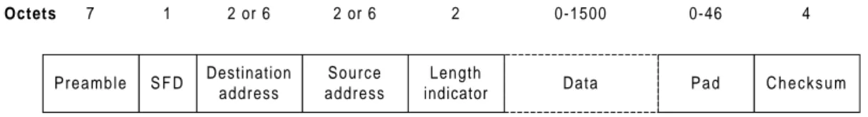
The IEEE 802.3 frame format is shown in Figure 2.5. Each transmitted frame has eight fields and is encoded using Manchester encoding (see [HAL96] for description of Manchester encoding). All fields are of a fixed length except from the data and pad fields.
Preamble Length Data P a d
indicator Source address Destination address S F D C h e c k s u m Octets 7 1 2 or 6 2 or 6 2 0-1500 0-46 4
Figure 2.5 The IEEE 802.3 Frame Format.
The preamble field is the first field of every frame. Its function is to allow the receiving MAC unit to achieve bit synchronization before the actual frame contents are received. The preamble field is 7 octets5, each containing the bit pattern 10101010. The second field is the start-of-frame delimiter (SFD) octet containing 10101011 to denote the start of the frame itself.
The destination and source addresses contain the identity of the intended destination DTE and the sending DTE, respectively. The standard allows for either 2 or 6 octets addresses, but for any particular LAN installation the size must be the same for all DTEs. The parameters defined for the 10-Mbps baseband standard use only the 6 octets addresses. The first bit in the destination address determines whether the frame is intended for a single DTE or a group of DTEs. If the bit is set to 0 it is an individual address and if it is set to 1 it is a group address. When a frame is sent to a group address, all the DTEs in the group receive it. Sending to a group of DTEs is called multicast. If the destination field contains only binary 1s, the frame is intended for all DTEs connected to the network. This is called broadcast.
The length field is a two-octet field indicating how many octets are present in the data field, from a minimum of 0 to a maximum of 1500 octets. IEEE 802.3 states that the minimum allowed frame size is 64 octets, from destination address to checksum. If the data portion of the frame is less than 46 octets, the pad field is used to fill out the frame to the minimum size. The maximum frame size is 1518 octets.
The final field is the checksum. It contains a four-octet CRC (cyclic redundancy check) value that is used for error detection.
2.2.3 Operation of IEEE 802.3
As mention earlier, the IEEE 802.3 uses CSMA/CD medium access control method. The CSMA/CD is used with bus and hub network topologies. With these topologies, all DTEs on the network are conceptually connected to the same cable which is said to operate in a multiple access (MA) mode. In this way all DTEs connected to the cable detect when a frame is being transmitted. A signal called a carrier sense (CS) signal is sensed at each DTE when the cable is occupied.
Frame Transmission
When a DTE has data to transmit, the data is first encapsulated into the format shown in Figure 2.5. The DTE then listens to the cable and checks whether it is being used
5
by anyone else, i.e., it checks whether a carrier signal is sensed. If the cable is idle, the DTE transmits its frame, but if the cable is occupied the DTE defers to any passing frame, and after a short additional delay called interframe gap (9.6 µs), the DTE transmits its frame. The purpose of the interframe gap is to allow the passing frame to be received and processed by the addressed DTE(s).
Frame Reception
When the destination DTE(s) detects that the frame currently being transmitted has its own address in the destination field of the frame, the frame contents comprising the destination and source addresses and the data field are loaded into a frame buffer to await further processing. During the reception a new checksum is calculated and then compared to the checksum field in the frame. If the checksums differ the frame is discarded. The frame is also discarded if it is too short or too long or if it does not contain an integral number of octets. If all these validation checks are in order, the frame is passed to higher sublayer for further processing.
Collision Detection
With this style of operation, it is possible for two DTEs (or more) to start transmitting at the same time after both detecting an idle cable. When this happens, the transmitted frames are said to collide on the network, resulting in corrupted frames. A DTE detects a collision by simultaneously monitoring the cable while transmitting. If the transmitted and monitored signals are different, a collision is assumed to have occurred. After a DTE detects a collision, it transmits a random bit pattern called a jam sequence to ensure that the duration of the collision is long enough to be noticed by all the other transmitting DTEs involved in the collision. The IEEE 802.3 requires that the jam sequence is at least 32 bits (but not more than 48). This guarantees that the duration of the collision is long enough to be detected by all transmitting DTEs on the network. After the jam sequence has been transmitted, the DTE terminates the transmission of the frame and schedules a retransmission attempt after a short randomly selected time interval. This random time interval is decided with an algorithm called the binary exponential backoff algorithm (see below).
Two very important aspects of collision detection are the maximum cable length and the minimum frame size. If a collision occurs, it is essential that a DTE transmitting a frame will detect the collision before ceasing its transmission. If the DTE has ceased transmitting its frame without detecting the collision, it draws the wrong conclusion that the frame has been successfully transmitted.
To ensure that a collision has not occurred the DTE must transmit long enough for the frame to propagate to all DTEs on the same segment. When each DTE on the segment has sensed a carrier no DTE will start transmitting and a collision is therefore avoided. In other words, a DTE cannot be sure that its frame has been successfully transmitted until it has transmitted for twice the worst case propagation delay, without detecting a collision. The reason that it must be twice the worst case propagation delay and not one is that if a collision occurs, the collided signal must propagate back to the transmitting DTE before it ceases its transmission.
The longest path allowed by IEEE 802.3 is 2.5 km and four repeaters. Given this maximum path length and that the bit rate is 10 Mbps, the worst case round trip propagation delay is 450 bit times [Bla93]. To be able to detect a collision, the minimum frame size must be larger than the sum of the worst case round trip propagation delay, 450 bits, and the maximum jam size, 48 bits. IEEE 802.3 adds a small safety margin and requires that the minimum frame size is 512 bits. Any frame
containing fewer than 512 bits is presumed to be a fragment resulting from a collision and is discarded by every receiving DTE on the network.
Binary Exponential Backoff Algorithm
As mentioned earlier, the binary exponential backoff algorithm is used to schedule a retransmission of a frame after a collision has occurred [Bla93]. The exponential backoff algorithm works as follows. After a collision, time is divided into discrete slots. This slot time is equal to the worst-case time delay a DTE must wait before it can reliably detect a collision, i.e., 512 bit times as described above. After the first collision, each DTE waits either 0 or 1 slot times before sending again. If a collision occurs again, each DTE will then wait either 0, 1 or 2 slot times. In general after k collisions, a random integer number between 0 and (2k-1) is chosen, and that number of slots is skipped before transmitting again. If ten collisions have been reached then the randomization interval is frozen at a maximum of 1023 slots (1023=210-1). This limit is known as the backoff limit. There exists also a limit called the attempt limit, which is set to 16. If the number of collisions have reached the attempt limit then the DTE in question will stop its retransmission attempts.
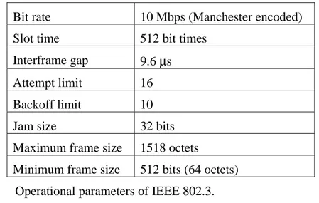
Table 2.2 summarizes the operational parameters given in the above description.
Bit rate 10 Mbps (Manchester encoded)
Slot time 512 bit times
Interframe gap 9.6 µs
Attempt limit 16
Backoff limit 10
Jam size 32 bits
Maximum frame size 1518 octets
Minimum frame size 512 bits (64 octets)
Table 2.2 Operational parameters of IEEE 802.3.
2.2.4 Example of a Collision
Here we give an example of a collision with 3 DTEs, A, B and C, where frames from A and B collide.
DTE A, detecting that the cable has been idle for 9.6 microseconds, begins transmitting its frame. While DTE A is transmitting, it is also monitoring the cable to be able to detect if a collision occurs.
D T E C
D T E B D T E A
1 0 1 0 1 0 1 0
Some period of time later, but before the signal from DTE A has had time to propagate down the cable to DTE C, DTE C also detects that the cable has been idle for 9.6 microseconds, and begins to transmit its frame. DTE C is also monitoring the cable.
D T E C
D T E B D T E A
1 0 1 0 1 0 1 0 1 0 1 0 1 0 1 0
At some point on the cable between DTE A and DTE C, the frames collide. As the signals continue to propagate, the corrupted frames travel down the cable
towards both DTE A and DTE C. D T E C
D T E B D T E A Collision
The DTE closest to the physical point on the cable where the two frames collided will detect the collision first. For the sake of this example, we will say that DTE A
detects the collision first. D T E C
D T E B D T E A
DTE A, detecting that a collision has occurred, immediately stops transmitting data and transmits a jam sequence onto the cable. DTE A will then use the Binary Exponential Backoff Algorithm to schedule a retransmission of the frame.
D T E C
D T E B D T E A
J a m S e q e n c e
Next, DTE C will detect the collision. DTE C will also send a jam sequence and implement the Binary Exponential Backoff Algorithm. D T E C D T E B D T E A J a m S e q e n c e
In the above example DTE B will discard the fragments resulting from the collision because they are less than 512 bits which is the minimum frame size allowed by IEEE 802.3.
2.3
IEEE 802.3u (Fast Ethernet)
Fast Ethernet is an appendum to the IEEE 802.3 standard [Hal96]. The standard is formally known as IEEE 802.3u and was officially approved by IEEE in June 1995. Fast Ethernet is also known as 100BaseT.
The 802.3 committee got the instructions from IEEE in 1992 to come up with a faster LAN. The committee came up with two proposals. One was to keep IEEE 802.3 exactly as it was, except from the bit rate, and the other one was to come up with a completely new standard, taking under consideration new factors, such as real-time traffic. The committee decided to use the first proposal. The people behind the other proposal formed their own committee which resulted in the IEEE 802.12 standard, also known as 100 (Base) VG-AnyLAN.
The aim of Fast Ethernet was to increase the speed over 10BaseT Ethernet (IEEE 802.3) without changing the wiring system, MAC method, or frame format. As mentioned in section 2.2.3 of IEEE 802.3, it is essential in a collision that a transmitting DTE has not ceased its transmission before detecting the collision. This is why the minimum frame size was set to 512 bits. Clearly, to be able to retain the
same minimum frame size at higher bit rates, the maximum path length must be reduced. This is the basis of the Fast Ethernet standard.
As can be seen from Table 2.1, the maximum segment length of 10BaseT is 100 m and hence the maximum distance between any two DTEs is 200m (DTE to hub to DTE). This means that the worst case path length for collision detection purposes is 400 m instead of the 5000 m specified in IEEE 802.3. This is how the Fast Ethernet standard can specify a bit rate at 100 Mbps.
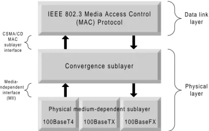
The protocol architecture of Fast Ethernet is shown in Figure 2.6.
I E E E 8 0 2 . 3 M e d i a A c c e s s C o n t r o l (MAC) Protocol C o n v e r g e n c e s u b l a y e r 100BaseFX 100BaseT4 100BaseTX Physical layer Data link layer C S M A / C D M A C sublayer interface M e d i a -i n d e p e n d e n t interface (MII)
Physical medium-dependent sublayer
Figure 2.6 Protocol architecture of Fast Ethernet
The convergence sublayer provides the interface between the IEEE 802.3 MAC protocol and the physical medium dependent sublayer. The purpose of the convergence sublayer is to make the use of higher bit rate and different media types transparent to the IEEE 802.3 MAC sublayer. To facilitate the use of different media types, the media independent interface (MII) provides a single interface that can support external transceivers for any of the 100BaseT physical sublayer. As we can see from Figure 2.6, the Fast Ethernet specification defines three separate physical sublayers, one for each media type [Tan96]:
• 100BaseT4 for four pairs of voice-or data-grade Category 3 UTP wiring.
• 100BaseTX for two pairs of data-grade Category 5 UTP and STP wiring.
• 100BaseFX for two strands of multimode fiber.
In the following sections these physical sublayers will be described.
2.3.1 100BaseT4
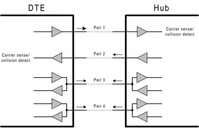
The 100BaseT4 physical sublayer uses category 3 UTP cable, consisting of 4 separate twisted pair wires [Hal96]. The main disadvantage of category 3 UTP cable is its limited clock rate, which is 30 MHz. To reduce the bit rate on each pair of wire, 100BaseT4 uses all four pairs to achieve 100Mbps in each direction. Of the four twisted pairs, one is always to the hub, one is always from the hub, and the remaining two are switchable to the current transmission direction (Figure 2.7). Collision is detected when a transmitting DTE (or hub) detects a signal on the receive pair.
Pair 1 Pair 4 Pair 3 Pair 2 D T E H u b Carrier sense/ collision detect Carrier sense/ collision detect
Figure 2.7 100BaseT4 use of wire pairs.
To achieve 100 Mbps with Manchester encoding using three pairs of wire, each pair must operate at 33.33 MHz. This clock rate exceeds the 30 MHz limit set by category 3 UTP cables. To reduce the clock rate, a code known as 8B6T is used instead of Manchester encoding. With 8B6T 6 ternary signal are used to represent 8 binary signals, i.e., prior to transmission, each set of 8 binary bits is first converted into 6 ternary symbols. In this way it is possible for each pair operate at 33.33 Mbps with a clock rate at only 25 MHz.
2.3.2 100BaseTX
100BaseTX is much simpler than 100BaseT4 because it uses category 5 UTP cables. The category 5 cable can handle clock rates up to 125 MHz [Tan96], compared to the 30 MHz of category 3. Because of this, 100BaseTX only uses 2 pairs of wires, one pair to receive data and the other pair to transmit data. Collision is detected if a signal is present on the receive pair during transmission.
Instead of using Manchester encoding as 10BaseT, 100BaseTX uses 4B5B encoding. When using 4B5B, every group of five clock periods is used to send 4 bits. Given a clock rate of 125 MHz and that 4B5B encoding is used, 100 Mbps can be achieved.
2.3.3 100BaseFX
100BaseFX uses 4B5B encoding scheme as 100BaseX and two strands of multimode fiber optic cable, one for transmission and one for reception. It was designed to allow segments of up to 412 meters in length. While it is possible to send signals over fiber for much longer distances, the 412 meters limit is to ensure that the propagation delay does not exceed the maximum allowed for collision detection.
3
Problem Description
This chapter gives a detailed description of the focus of this project, i.e., designing switched networks. We will begin in section 3.1 by giving an introduction to the evolution of network usage the past decade. Because of this evolution, many of today’s networks are stressed to their limits. One promising solution to this is switching technology. We describe the advantages of using switches in section 3.2. The new functionality of switching technology sets new requirements on network design and planning. In section 3.3 we identify the problems of designing switched networks and discuss how we intend to tackle them in the rest of the project.
3.1
Changing Requirements
Use of information technology has undergone a radical change in the last decade. The purpose of this section is to give an insight into the changes that have occurred affecting data communication structures and traffic patterns.
3.1.1 The Move to Server Centralization
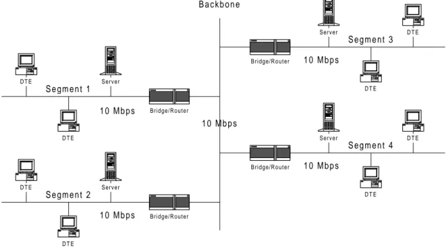
Figure 3.1 shows a typical network design as it was several years ago. The network is divided into segments with bridges and/or routers and all the segments were connected together through the backbone. Usually the backbone had the same bandwidth as the segments. Because of the limited capacity of the backbone, each segment had its own servers to minimize traffic to other segments.
D T E D T E D T E D T E D T E D T E D T E D T E B a c k b o n e S e g m e n t 1 S e g m e n t 4 S e g m e n t 3 S e g m e n t 2 1 0 M b p s 1 0 M b p s 1 0 M b p s 1 0 M b p s 1 0 M b p s Server Server Server Server Bridge/Router Bridge/Router Bridge/Router Bridge/Router
Figure 3.1 Typical network design a few years ago
This design works fine for relatively small networks with few segments. But in organizations with many segments it becomes difficult to manage a large number of servers in possibly unsecured locations around the building or campus.
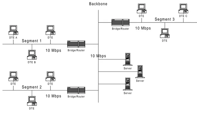
This has led to the centralization of servers, i.e., grouping of servers in one physically secure location with network links between all users and the server room (see Figure 3.2). The servers are typically connected directly to the backbone.
D T E A D T E B D T E D T E D T E D T E D T E C D T E B a c k b o n e S e g m e n t 1 S e g m e n t 3 S e g m e n t 2 1 0 M b p s 1 0 M b p s 1 0 M b p s 1 0 M b p s Server Server Server Bridge/Router Bridge/Router Bridge/Router D T E
Figure 3.2 Centralized servers
With all servers located in one place, the administration becomes much easier. Issues such as reliability, security and disaster recovery can easily be fulfilled. The server room can, e.g., be equipped with redundant back-up power supplies and halogen fire protection, etc.
This migration to centralized client/server architecture has completely changed the traffic pattern on the network. Network designers no longer have the luxury of assuming that the clients will mainly be connecting to local resources as before. Now all traffic to the servers must go through the network’s backbone. This means that the backbone’s capacity must increase significantly in order to cope with the increased traffic. Unfortunately most of the today’s backbones have not been built with this in mind and have therefore become a bottleneck in many networks.
3.1.2 Universal IT Trends
Apart from the migration to centralized client/server architecture, there are a few universal IT trends that most organizations are subjected to. These will be covered now.
Growth of connected users.
The number of connected users is constantly growing. According to an estimate by Matrix Information and Directory Services (MIDS), one of the foremost sources of Internet demographics (see www.mids.org), the Internet has about 57 million users as of January 1997. A user is a user of a computer that can access information by interactive TCP/IP services such as WWW or FTP. According to MIDS, the Internet is approximately doubling in size each year. MIDS estimates that the number of users will grow with the current rate for at least 3 more years resulting in over 700 million users in 2001 (see Table 3.1)
Jan 1990 Jan 1997 Jan 2000 Jan 2001
1,120,000 57,000,000 377,000,000 707,000,000
Table 3.1 Past, present, and future projections.
Even though these numbers only apply to users connected to the Internet and not the number of users connected to a local area network (LAN), they give a good insight over where we are heading, i.e., the number of users is neither constant nor reducing but continuously increasing.
Traffic volume increases per user.
A parallel trend is that the traffic volume increases, even across a fixed number of users. One reason for this is the ever-increasing use of Web browsers. Due to their simple and intuitive user interface, the average non-technical person understands almost immediately how to use a browser to navigate trough the Internet and intranet, even with no training. Taking advantage of the Web browser’s simplicity, many organizations are already implementing intranets using the World Wide Web technology. Intranets are generally expected to generate new traffic on the corporate network.
The growth in size and types of data used by new applications has also contributed to the increased traffic volume. The use of large files such as multimedia, video, and voice is constantly growing. Usage of conferencing applications is also increasing adding new requirement on the network. Different from normal data, these applications are highly sensitive to network delay.
More powerful computers.
One interesting trend is that many organizations regularly upgrade their computers to answer new demands made by new applications, but leave the network as it is. Today’s computers demand large amount of bandwidth and can easily exceed Ethernet’s 10 Mbps limit. The throughput limitation on a server is the limited bandwidth available to it and therefore the network becomes a bottleneck in client/server architecture. To be able to utilize the new computers the network must also be upgraded. High performance computers need high performance networks if anyone expects to derive benefits from them.
3.1.3 Old Solutions
It is very difficult to meet new demands with the traditional building blocks but there exist a few methods. Two of them are described here and their advantages and disadvantages pointed out.
LAN segmentation
As conventional shared LANs become congested, there are not many ways of increasing the network bandwidth. One popular technique is LAN segmentation. LAN segmentation utilizes that bridges and routers can filter traffic received on a shared LAN interface and forward frames to other LANs only when necessary. By utilizing this functionality it is possible to split an overloaded LAN in half. The traffic load on each of the new segments is then less than of the single segment. Consider a LAN with 10 DTEs (see Figure 3.3). Each DTE gets 1/10 of the available bandwidth. By dividing the segment in two smaller segments of 5 DTEs each, each DTE gets 1/5 of
the available bandwidth. As the network is split into smaller and smaller segments, each containing fewer DTEs, each DTE gets more bandwidth.
D T E D T E D T E D T E D T E D T E D T E D T E D T E D T E Before Segmentation D T E D T E D T E D T E D T E D T E D T E D T E D T E D T E After Segmentation Router/bridge
Figure 3.3 LAN segmentation
While effective at first, LAN segmentation eventually grows too complex and too expensive. When the number of routers increase, the network becomes difficult to manage. A simple operation such as moving a DTE to another subnet may require address reconfiguration in each router. Moreover, when a DTE must communicate outside of its local segment the data may have to pass several routers or bridges to reach its destination and therefore adding further to the network latency. Finally router ports are designed and priced for large numbers of DTEs and therefore cost per DTE grows to unacceptable levels when using LAN segmentation.
FDDI backbone
When migrating to centralized client/server architecture, the requirement on the available bandwidth to the server increases. Taking advantage of FDDI’s 100 Mbps channel capacity, many network managers have connected their centralized servers on a shared media FDDI backbone. This solution works fine for small networks, but the problem is that the aggregate bandwidth of FDDI remains constant at 100 Mbps regardless of the number of attached DTEs. Therefore it is not scalable to medium and large networks with many servers connected to the backbone. The bandwidth to each server can be increased as in LAN segmentation by splitting the FDDI ring into multiple, smaller FDDI networks joined by a router with multiple FDDI interfaces, but as in LAN segmentation this is only a temporal solution.
3.1.4 The Effect on the Networks
All these changes in today’s networking we have mentioned so far are outpacing existing networks’ abilities to support them. The traditional building blocks are not adequate to deal with the increased traffic load. The networks are falling behind!
3.2
Switching – a new Networking Paradigm
Switching is a new technology paradigm in networking. Switching technology is currently available in two forms [Bay95a]: frame switching and cell switching. The difference between these is that frame switches move frames rather than cells. Frames can vary from a few bytes to thousands of bytes depending on MAC method (IEEE 802.3 frames are from 65 bytes to 1518), but cells are always the same size (ATM cells are always 53 bytes)
Since this project only focuses on switching in IEEE 802.3 we will only cover frame switching in this chapter.
3.2.1 Frame Switching
A frame switch operates much like a multiport bridge. By examining the source address of each received packet, the switch creates a table containing addresses of all DTEs attached to each of its ports. Once this has been done, the switch can check the destination address in each received frame and forward it only to the port(s) to which it is addressed. The output port may be attached directly to a DTE, to a shared segment with multiple DTEs, or to another frame switch which, in turn, is connected to the destination. Frame switches forward traffic based on one of two forwarding models [Bay95b]:
• Cut-through switching
• Store-and-forward switching
Cut-through switches start forwarding frames before the entire frame is received. The switch does only need to read to the destination MAC address before it begins forwarding the frame. In this way frames are processed faster therefore introducing lower latency. The major disadvantage with cut-through switches is that they do not detect corrupted frames like too small frames and frames with FCS-errors. These frames are forwarded to the destination despite of the errors. A store-and-forward switch, however, reads and checks each frame for errors before forwarding it. Erroneous frames are therefore detected and not forwarded to their destinations. This buffering of frames imposes a latency penalty on all frames based on their length. Store-and-forward switching enable switches to establish a communication link between ports of differing speeds. Fast ports must wait for the entire frame from a slow port in order not to underrun the transmission, and a slow port cannot receive a frame at the rate a fast port transmits it. This enables the use of both 10 Mbps IEEE 802.3 (Ethernet) and 100 Mbps Fast Ethernet on the same switch.
Another advantage of a switch over a bridge is that a switch can establish multiple communication channels between ports and exploit parallel communication [Hal96]. Consider 4 DTEs, A, B, C and D where A is communicating with C, and B is communicating with D (see Figure 3.4). With the functionality of switches both connections can be active simultaneously. With multiport bridges only one connection can be active at the same time.
D T E A
D T E B D T E D D T E C Inside a switch
Figure 3.4 Simultaneous links between pairs of communicating devices
If we have a frame switch with 16 10 Mbps IEEE 802.3 ports we could optimally establish 8 active communication channels in the switch resulting in a total bandwidth of 80 Mbps. In this way can a switch with n ports give n/2*bit rate bandwidth in optimal use. Therefore when connecting a DTE or a shared segment with multiple DTEs to a switch the overall throughput of the network increases.
In addition to these benefits, the use of application-specific integrated circuit (ASIC) technology allows a switch to provide greater performance than a traditional bridge by supplying high frame throughput with extremely low latency.
3.3
Designing Switched Networks
Switching technology is a new technology and requires new ways of designing and planning networks. When connecting a new DTE to a traditional shared network, it does not matter where it is connected, i.e., on which port of the hub or where on the coaxial cable, as long it is on the right subnet. This is not the case of switched network. The location of the new DTE becomes very important. To be able to connect the DTE you must know exactly how the network looks like, where the servers are located, where the clients are, and which client communicates with which server. These requirements add much strain on the network administrator.
Unfortunately there is a lack of information for how to design switched networks. It is the intention of this project to give an insight in how to design switched networks. To do that we will do benchmark tests on a few different network architectures. After doing these tests we shall be able to evaluate the effects of introducing a switch in a network and how it is best utilized in client/server architecture. The benchmark tests are described in chapter 4.
4
Testing Methodology
As we mentioned in chapter 3, we are going to do benchmark tests on a few different network architectures. In this chapter we describe how these benchmark tests are performed. We begin in section 4.1 by presenting the architectures that will be used. In section 4.2 we list the hardware that will be used and in 4.3 we describe the software we use to generate traffic on the network. Finally in 4.4, we describe our simulation settings.
4.1
Architectures
As with every design there are million different solutions, where the design may range from complicated to simple. Simplicity is very important in the selection of the architectures we will use. It can be very difficult to interpret the results if there are many factors that affect the result.
In our benchmark tests we will have nine clients and one server and measure the throughput on the network over a few different architectures. In the selection of the architecture we focus on showing the effect of introducing a switch into a shared network. We therefore begin by doing a benchmark test on a shared network where all the computers are connected to a hub. This architecture serves as a reference for the other benchmark tests. We then do benchmark tests on three other architectures. In each architecture, the clients communicate with the server through a switch, but the difference being the distribution of the clients. We go from all clients connected to the same port of the switch to each client connected to its own port.
The architectures are described in detail in the following sections.
4.1.1 Shared 10 Mbps
This architecture acts as a reference for the other benchmark tests. All the clients and the server connect to the same shared media. All are operating at 10 Mbps.
The physical connection is as in Figure 4.1. We use two 8 port hubs to connect all the computers together.
Client
Client Client Client Client Client
Client Client Client Server
H u b H u b
Figure 4.1 Shared 10 Mbps
4.1.2 All Clients on one Port of a Switch and the Server on another Port
There is a common misunderstanding that to increase the throughput on the network it is sufficient to connect the server to one port of a switch and all the clients on another port. Given that all the clients are communicating with the server and no client is communicating with another client, adding a switch should add to network latency. We should get a worse throughput than using a shared 10 Mbps. The reason for this is that the server can only be serving one client at a time, therefore not utilizing the
parallel functionality of the switch. It should not matter whether the server is connected to the switch at 10 Mbps or 100 Mbps, because there is only one client active at a time.
The physical connection is presented in Figure 4.2. We will run the test two times where the server connected at 10 Mbps in the first run and at 100 Mbps in the second.
Server
Client
Client Client Client Client Client
Client Client Client
H u b H u b
10/100 Mbps Switch
Figure 4.2 All clients on one port and the server on another
4.1.3 3 Clients on 3 Ports and Server on one Port
Here we will split the nine clients in three groups, each containing three clients. Each group is connected to a hub which is then connected to one port of the switch. The server is connected to a separate port on the switch (see Figure 4.3). We will run the test twice as before, once with the server at 10 Mbps and once at 100 Mbps. In this case we should get better throughput as we have begun to exploit the parallelism of the switch.
Server
Client
Client Client Client Client Client
Client Client Client
H u b H u b 10 Mbps 10/100 Mbps Switch H u b 10 Mbps 10 Mbps
Figure 4.3 3 clients on 3 ports and the server on another
4.1.4 All Clients on separate Ports and Server on one Port
This is the extreme case where each client is connected directly to the switch at 10 Mbps. The server connected to a separate port. The test will be run two times as before. Now we fully utilize the parallelism of the switch. We should get a considerable increase in throughput when running the server at 100 Mbps.
Server
Client
Client Client Client Client Client
Client Client Client
10/100 Mbps Switch
Figure 4.4 All clients on separate ports and the server on one port
4.2
Hardware
The hardware we use is presented in Table 4.1.
Hardware Description
9 clients Each client has a 100 MHz 486DX4 Intel processor, 12 Megabyte RAM and 10 Mbps 3com Etherlink III NIC for ISA.
1 server The server has a 133 MHz Pentium Intel processor, 24 Megabytes Ram and a 10/100 Mbps 3com Etherlink XL NIC for PCI.
3 hubs The hubs are all from Allied Telesis (CentreCOM
MR820T) with 8 10BaseT ports and one AUI port.
1 switch The switch we use is Model 28115 LattisSwitch Ethernet Switching Hub from SynOptics. The switch forwards traffic based on the store-and-forward model. The switch has 16 dual-speed 10BaseT or 100BaseTX attachment ports and two expansion ports. We will use 10 of the attachment ports.
media All the computers are connected to the network with
Category 5 Twisted Pair cables.
Table 4.1 The hardware used in the performance test.
4.3
Perform3
Perform3 is a well-known benchmarking program provided by Novell to measure network throughput produced by memory-to-memory data transfers from a file server to participating test workstations. Perform3 works under any network operating system that allows DOS files to reside on the file server. The program is available from Novell at no charge.
4.3.1 Detailed Description
For perform3 to work we need a file server and one or more clients. In our case we have a Novell NetWare 4.11 server and 9 DOS clients (Novell NetWare Requester CLIENT32.NLM v2.01). As there is no documentation available for Perform3 we shall describe in detail how it works. This description is based on our experience. We begin by logging on the server from the clients. We then execute Perform3 locally on all the clients. The first client that runs Perform3 creates a synchronization file called perform3.syn for the other clients to watch. Note that if the other clients are to
be able to see the synchronization file then Perform3 must be executed from the same current directory on all clients, i.e., a network drive on the server. As each client watches this synchronization file, the test can be started on all clients simultaneously from the first client that executed Perform3. When the test starts, each client starts to read a file of a given size from the server. The bulk of the data transfer is therefore only flowing from the server to the clients.
Perform3 allows us to set several parameters:
• Duration (12 to 65535 seconds)
• Start size (1 to 65535 bytes)
• Stop size (start size to 65535 bytes)
• Step size
When we start the test each client begins by reading a file of start size bytes from the server. Each client repeatedly read a file of this size for duration seconds. When that time has elapsed the file size is increased by step size bytes and again repeatedly read from the server for duration seconds. This procedure is then repeated till we have reached the stop size.
One of the advantages of using Perform3 is that it uses file server disk caching to ensure that there is no disk activity during the timed portions of a test. By pre-caching the data requested by each client, the test permits the server’s and the clients’ network adapters to operate at peak performance, without having to wait for the server’s hard disk to read or write data.
The performance data reported by Perform3 is the average throughput on the network during each interval. The throughput is calculated on each client and the aggregate throughput of all clients is calculated by the first client that executed Perform3 (see Table 4.). File Size (bytes) This station (KBps) Aggregate throughput (KBps) 1432 120,78 1087,04 1254 119,34 1074,07 1076 117,16 1054,40 898 109,62 986,61 720 103,24 929,14 542 100,43 903,89 364 84,82 763,38 186 66,46 598,17 8 4,61 41,52
Table 4.2 Performance data given by the first client during one test.
4.4
Simulation Settings
As we have described there are four different parameters that can be given to Perform3. We have selected to start with a file size of 8 bytes and increase the file
have tested 9 different IEEE 802.3 frame sizes. The reason for why the maximum file size tested is only 1432 bytes and not 1518 bytes (the maximum frame size allowed by IEEE802.3) is that the 1432 bytes is not the size of the actual frame sent on the media. 1432 bytes is the size of the file that is read from the server. Figure 4.5 shows a simplified description of this. The Novell server and the clients communicate through a protocol called IPX. The file that is read from the server is therefore encapsulated in an IPX frame. The IPX frame is then encapsulated in an IEEE 802.3 frame before it is actually sent on the network.
Data IPX-frame
Header F C S
22 octets 4 octets
IEEE 802.3 frame
The actual file size Header
Figure 4.5 Simplified figure of the actual frame size sent on the network
With a simple test that we did with the aid of Perform3 we could determine that when a file of 1432 bytes was read from the server we actually sent a frame of 1518 bytes over the network. The additional headers and control data introduced by upper layer protocols produce an overhead of 86 bytes when reading a file of 1432 bytes.
It is very important to keep this in mind when reading the performance data given in next chapter. When the file read over the network is as small as 8 bytes the additional overhead has much more effect on the throughput than with larger files. If a client is reading a file of 8 bytes the actual frame size on the network can be as large as 94 bytes. The performance data is calculated based on the total bytes read from the server, but not the bytes sent on the network. We should therefore expect a very low throughput when reading small files.
5
Analysis
In this chapter we will present the results of the benchmark tests we performed. In sections 5.1 to 5.4 the results from each of the tests are given. In section 5.5 the results are compared to each other and in 5.6 we will discuss the correctness of the test. Finally in 5.7 the design guidlines are given. All the graphs we present are based on the performance data given in Appendix A. For a description of the different architectures see section 4.1.
5.1
Shared 10 Mbps
As we described in section 4.1 this architecture serves as a reference for the other architectures. The graph below summarizes the results from the benchmark test.
Average throughput 0,00 20,00 40,00 60,00 80,00 100,00 120,00 140,00 8 186 364 542 720 898 1076 1254 1432
File size (bytes)
K
Bp
s
The graph shows how the average throughput per client changes when the file size is increased. As we expected, the throughput is very low when the file is small because of the overhead introduced by the protocols used to transfer the file. The reason for this is that the overhead introduced by upper layer protocols is always constant, i.e., the same number of octets each time a file is transferred. When the file read over the network becomes smaller the overhead will become larger in proportion to the file, resulting in worse throughput.
Another aspect that can explain this low throughput with small files is that when the frames are small the chance of a collision occurring increases. This is discussed in more detail in section 5.6.
It is very interesting to notice how fast the throughput increases when the file size becomes larger. While the file size increases from 542 bytes to 1432 bytes, i.e., by 164%, the throughput only increases from 100,43 KBps to 120,78 KBps or 20%. This means that already when the file size is 542 bytes the throughput has almost reached its maximum.
By calculating the average throughput of the graph above we get the average throughput of each client over the different file sizes. The outcome of that is 91,83 KBps.
The only computer the clients are communicating with is the server. The clients do not communicate with each other. Given the above we can calculate the throughput of the server by calculating the aggregate throughput of all the clients. The average throughput of the server is then 826,47 KBps (91,83*9).
5.2
All Clients on one Port of the Switch and the Server on Another
The graph below shows the average throughput of the clients when the server is connected to the switch at 10 Mbps.
Average throughput 0,00 20,00 40,00 60,00 80,00 100,00 120,00 8 186 364 542 720 898 1076 1254 1432
File size (bytes)
K
Bp
s
The graph is very similar to the graph in 5.1 Shared 10 Mbps. The throughput increases from 91,91 KBps to 111,46 KBps or 21% while the file size increases from 542 bytes to1432 bytes, compared to 20% in 5.1. The average throughput over the different file sizes is however lower or 85,46 KBps. This shows that introducing a switch as in this architecture has negative effect on the throughput. The switch adds to the network latency. The throughput of the server is 769,13 KBps or 6,9% less than in 5.1.
The graph below shows the results of a benchmark test exactly as the one above, but the server is now connected to the switch at 100 Mbps instead of 10 Mbps.
Average throughput 0,00 20,00 40,00 60,00 80,00 100,00 120,00 8 186 364 542 720 898 1076 1254 1432
File size (bytes)
K
Bp
s
The throughput to the clients is 84,17 KBps, just under the throughput when the server is connected at 10 Mbps. This is a very interesting result. This shows that the bottleneck in this architecture is the 10 Mbps connection to the clients. The difference between the two tests, i.e., the server at 10 Mbps and the server at 100 Mbps is insignificant. When the server is connected at 100 Mbps the throughput is only 1,5% less than when the server is on 10 Mbps. There can be a few reasons for this difference. One can be that converting from 10 Mbps to 100 Mbps can add to latency.
5.3
3 Clients on 3 Ports and the Server on one Port
In this testrun we begin to utilize the parallelism of the switch as the clients are distributed on three different ports. The graph below shows the results from the test when the server is connected at 10 Mbps.
Average throughput 0,00 20,00 40,00 60,00 80,00 100,00 120,00 140,00 8 186 364 542 720 898 1076 1254 1432
File size (bytes)
K
Bp
s
The throughput increases by 19% when the file size goes from 542 bytes to 1432 bytes which is a little less than with the shared 10 Mbps. Now the parallelism of the
switch has begun to win up the additional latency introduced by the switch. The throughput to the clients is now 93,82 KBps or only 2% better than with shared 10 Mbps. The 10 Mbps connection to the server has obviously become the bottleneck of this architecture. The graph below shows what happens when the connection to the server is increased from 10 Mbps to 100 Mbps.
Average throughput 0,00 50,00 100,00 150,00 200,00 250,00 300,00 350,00 8 186 364 542 720 898 1076 1254 1432
File size (bytes)
K
Bp
s
Now we have begun to see some significant improvements. The average throughput to the clients is now 235,89 KBps or 157% better than with shared 10 Mbps. The connection to the server is not the bottleneck anymore. The throughput increases however at higher rate when the file size increases compared to shared 10 Mbps. The throughput goes from 253,49 KBps with file size at 542 bytes to 326,11 KBps at 1432 bytes which is 29% increase compared to 20% with shared 10 Mbps.
5.4
All Clients on Separate Ports
The architecture we test here is the extreme case of using switches. Each client is connected to its own port of the switch. The graph below shows the result from the test where the server is connected at 10 Mbps.
Average throughput 0,00 20,00 40,00 60,00 80,00 100,00 120,00 140,00 8 186 364 542 720 898 1076 1254 1432
File size (bytes)
K
Bp
s
The average throughput of the server is almost exactly as the test in 5.3 where the clients are distributed on 3 ports and the server at 10 Mbps. Here the average throughput is 93,80 KBps where it was 93,82 KBps in the other test. As with the test in 5.3 the 10 Mbps connection to the server is again the bottleneck of this architecture. In the next graph the connection to the server has been increased to 100 Mbps.
Average throughput 0,00 100,00 200,00 300,00 400,00 500,00 600,00 8 186 364 542 720 898 1076 1254 1432
File size (bytes)
K
Bp
s
The first thing we notice about this graph is how fast the throughput increases when the file size increases. The throughput increases from 283,89 KBps at 542 bytes to 487,97 KBps at 1432 bytes or 72%. The average throughput to the clients is 309,54 KBps, which is 237,08% better than in shared 10 Mbps.
5.5
Summary
It is quite interesting to notice that introducing a switch in client/server architecture as we tested has almost no effect as long as the server is connected at 10 Mbps. The graph below shows this clearly.
Average throughput 0,00 100,00 200,00 300,00 400,00 500,00 600,00 8 186 364 542 720 898 1076 1254 1432
File Size (bytes)
K Bp s Test1 10Mbps Test2 10Mbps Test2 100Mbps Test3 10Mbps Test3 100Mbps Test4 10Mbps Test4 100Mbps
In the graph, Test1 refers to shared 10 Mbps, i.e., section 5.1, Test2 refers to 5.2, etc. All the architectures with the server connected at 10 Mbps appear in the bottom of the graph. The 10 Mbps connection to the server is clearly the bottleneck in this client/server architecture.
We have also shown that connecting the server at 100 Mbps does not always increase the throughput. In Test 2 when we changed the connection to the server from 10 Mbps to 100 Mbps, it had no effect on the throughput. In that case the 10 Mbps connection the clients was the bottleneck. This is naturally an extreme case but it shows that it is very important to know which clients are communication to which servers and where they are physically connected to the network.
It is also interesting to see how the difference in throughput between tests gets smaller when the file size is small. By looking at the two tests where the server was connected at 100 Mbps, i.e., Test 3 and Test 4, we notice that the difference decreases when the file size gets smaller and is almost zero when the file is 364 bytes. Test 3 is then only 5% less than Test 4, compared to 33% when the file is 1432 bytes. It is very difficult for us to point out the reasons for this as there are many factors that can affect this, e.g., the maximal forwarding rate of the switch (frames per seconds) or the maximal frames per seconds transmitted by the Ethernet card in the server. We can however see that when the file size has reached 364 bytes it does not matter whether the clients are distributed at 9 ports or 3. We can therefore draw the conclusion that the connection to the server has become the bottleneck at this stage.
The graph below summarizes the result of all the benchmark tests. It shows the average throughput of the clients in each test.
Average throughput of clients 0 50 100 150 200 250 300 350 Test1 10Mbps Test2 10Mbps Test2 100Mbps Test3 10Mbps Test3 100Mbps Test4 10Mbps Test4 100Mbps KBps
5.6
Correctness of the Test
As we mentioned in chapter 4, all the clients had the same type of network cards (10 Mbps 3com Etherlink III NIC). The reason for this is that we wanted the clients to be as similar as possible. Despite of this it is possible that one or more of the network cards we used were erroneous and therefore resulting in worse throughput on the client in which they were located. To analyze whether this occurred in our benchmark tests we have summarized the throughput of each client in the following graph:
Average throughput per client
0 20 40 60 80 100 120 140 160 Client1 Client2 Client3 Client4 Client5 Client6 Client7 Client8 Client9 Average KBps
The graph shows the average throughput of each client over all the benchmark tests we performed. As we can see there was no client that got significantly more throughput than another. The difference between the lowest (Client 9) and the highest
(Client 3) is only 6%, i.e., the throughput of Client 9 was 6% less than of Client 3. This implies that none of the network cards we used were erroneous.
Another interesting aspect about our results is the low throughput we attained when the file read over the network was small. We have already described one possible reason for this, i.e., overhead from upper layer protocols (see section 4.4), but we have not discussed this in relation to collisions. This will be done in the rest of this section.
As the file read over the network becomes smaller, then the time it takes to send the file decreases. This means that more frames can be sent over the network when the file is small. The graph below shows this clearly.
Average number of frames
0 500 1000 1500 2000 2500 3000 3500 8 186 364 542 720 898 1076 1254 1432
File size (bytes)
F
rames per secon
d
The graph shows the number of frames per second the server sent during the benchmark test when all the clients were connected to one port of the switch and the server on another (see section 5.2). The number of frames per second decreases by 78% when the file size increases from 8 bytes to 1432 bytes.
When the number of frames decreases then the chance of a collision occurring also decreases (for further description of a collision see section 2.2.3 and 2.2.4). When a collision occurs the frames involved in the collision will collide and their contents will therefore be corrupted. After the collision is detected than each computer involved in the collision will schedule a retransmission of their frame. During this period, i.e., from the occurrence of the collision, to the detection of the collision and finally to the retransmission of the frames, no data has been sent on the network. Even though the network is active, i.e., bits are being transmitted, the network is in fact idle in terms of data transmission.
Based on the description above we can draw the conclusion that the number of collisions was higher when the file was smaller, resulting in more idle time on the network, which in turn resulted in worse throughput.
5.7
Design Guidelines
Based on the benchmark tests that we have performed, i.e., client/server architecture where the clients do not communicate with each other and the main traffic stream is from the server to the clients, we can recommend the following:
• Connect the server to the switch at 100 Mbps.
• Distribute the clients on more than one port of the switch. The more distribution the better throughput.
Although we have not tested other traffic patterns we can recommend a few guidelines:
• If clients communicate with each other – group those clients together in a way that most of the traffic in each group is local. Then connect each group to one port of the switch. In this way the traffic between clients in one group will not propagate to other clients in another group.
• If the clients are communicating with one or more servers – connect each server to the switch at 100 Mbps.