Autonomous Mobile Robot Cooperation

Autonomous Mobile Robot Cooperation

(HS-IDA-EA-97-109)

Ásgrímur Ólafsson (a94asgol@ida.his.se)

Department of Computer Science

Högskolan i Skövde, Box 408

S-54128 Skövde, SWEDEN

Final Year Project in Computer Science, Spring 1997.

Supervisor: Tom Ziemke

Autonomous Mobile Robot Cooperation

Submitted by Ásgrímur Ólafsson to Högskolan Skövde as a dissertation for the degree

of BSc, in the Department of Computer Science.

1997-08-12

I certify that all material in this dissertation which is not my own work has been

identified and that no material is included for which a degree has previously been

conferred on me.

Autonomous Mobile Robot Cooperation

Ásgrímur Ólafsson (a94asgol@ida.his.se)

Key words: Artificial neural networks, Obstacle avoidance, Mobile robots,

Cooperation, Communication

Abstract

This project is concerned with an investigation of simple communication between

ANN-controlled mobile robots. Two robots are trained on a (seemingly) simple

navigation task: to stay close to each other while avoiding collisions with each other

and other obstacles.

A simple communication scheme is used: each of the robots receives some of the

other robots’ outputs as inputs for an algorithm which produces extra inputs for the

ANNs controlling the robots.

In the experiments documented here the desired cooperation was achieved. The

different problems are analysed with experiments, and it is concluded that it is not

easy to gain cooperation between autonomous mobile robots by using only output

from one robot as input for the other in ANNs.

Table of Contents

1

Introduction ... 1

1.1

The problem domain... 1

1.2

Purpose ... 1

2

Background ... 2

2.1

Robots... 2

2.2

Artificial neural networks ... 3

2.2.1 Network structures... 5

2.2.2 How do the ANNs work... 6

2.2.3 Learning in ANNs... 6

2.2.4 Why use ANNs ? ... 7

2.3

Related work ... 7

2.3.1 Work related to communication schemes and cooperation... 8

2.3.2 Work related to multiple robots... 9

3

The simulator ... 10

3.1

Description of the world ... 11

3.2

Description of the robot ... 11

3.2.1 Distance sensors... 12

3.2.2 Blind areas ... 12

3.2.3 Motors ... 13

4

Problem description... 14

4.1

Activities which the robots have to accomplish... 16

4.2

A number of factors that will be studied ... 16

4.3

A number of factors that will not be studied... 16

4.4

Expected results ... 16

5

Method... 17

5.1

Choice of ANN architecture ... 17

5.2

Choice of learning method... 17

5.2.1 Reinforcement Learning... 17

5.2.1.1 How reinforcement learning works ... 18

5.2.1.2 Possible rewards and penalties for the robot ... 18

6

Changes made to the simulator ... 21

6.1

Changes made to the robot ... 21

6.2

Changes made in the robot part of the screen ... 21

6.2.1 Changes that can be seen... 22

6.2.2 Changes that can not be seen... 23

7

Implementation ... 24

7.1

Experiment 1 ... 24

7.1.1 The aim... 24

7.1.2 The network... 24

7.1.3 The values for the learning function ... 25

7.1.4 Result from experiment 1... 26

7.1.5 How experiment 1 works ... 26

7.1.6 Learning in different worlds... 27

7.2

Experiment 2 ... 28

7.2.1 The aim... 28

7.2.2 The network... 28

7.2.3 Result for experiment 2... 29

7.3

Experiment 3 ... 29

7.3.1 The aim... 30

7.3.2 The network... 30

7.3.3 The algorithm ... 30

7.3.4 Result for experiment 3... 31

7.3.5 Learning in different worlds... 31

7.4

Experiment 4 ... 32

7.4.1 The aim... 32

7.4.2 The network... 32

7.4.3 Result for experiment 4... 32

8

Overall results ... 33

8.1

Activities which the robots had to accomplish ... 33

8.2

A number of factors that were also studied ... 33

9

Conclusion ... 34

9.1

Future work... 34

9.1.1 Make independent algorithm... 34

9.1.2 Add more robots to the simulator ... 34

Acknowledgments ... 35

References ... 36

Appendix A ... 37

Appendix B... 42

Appendix C ... 43

Appendix D ... 44

Appendix E... 45

Appendix F ... 50

Appendix G ... 52

Appendix H ... 59

Appendix I... 60

Appendix J ... 67

Appendix K ... 71

Appendix L... 72

Appendix M... 74

Appendix N ... 78

1

Introduction

This document contains a description of a final year project in computer science at the

University of Skövde.

This chapter will briefly describe the problem and why it is interesting to study.

1.1

The problem domain

In this project multiple robots are supposed to cooperate using Artificial Neural

Networks (ANNs). Two robots are trained on a simple navigation task, i.e. to stay

close to each other while avoiding collisions with each other and other obstacles. This

study will show how to use the output from one robot as input for the others and vice

versa to achieve the desired coordination, i.e. using simple communication schemes.

Figure 1.1: This figure is an example of how output from one robot

could/can be used as input for another. To gain more understanding of the

figure read the chapter about ANNs (chapter 2.1).

1.2

Purpose

The intention of this project is to study how cooperation between autonomous mobile

robots can be achieved using only simple communication schemes.

Many people believe, according to Huber and Kenny [Hub94], that it will be common

in the near future to see autonomous robots working in teams and as separated

individuals. Each of these robots has to do its own task and if it will need any

assistants to accomplish some task it will have to cooperate with other robots or

humans.

Communication is, according to Moukas and Hayes [Mou96], a prerequisite for

cooperation, which is a prerequisite for intelligent social behavior. Saunders and

Pollack [Sau96] argue that the role of communication in multi-agents systems is one

of the most important open issues in multi-agent system design.

N e t w o r k f o r

R o b o t 1

N e t w o r k f o r

R o b o t 2

O u t p u t u n i t H i d d e n u n i t I n p u t u n i t I n p u t u n i t I n p u t u n i t I n p u t u n i t H i d d e n u n i t H i d d e n u n i t O u t p u t u n i t

( M o t o r 1 )

O u t p u t u n i t H i d d e n u n i t I n p u t u n i t I n p u t u n i t I n p u t u n i t I n p u t u n i t H i d d e n u n i t H i d d e n u n i t O u t p u t u n i t

( M o t o r 2 )

( M o t o r 1 )

( M o t o r 2 )

2

Background

In this chapter robots and ANNs will be described. Related previous work will also be

presented.

2.1

Robots

More than centuries ago man has dreamed of robots, and many people have tried to

make robots in some form. According to McKerrow [McK91] the ancient Egyptians

attached mechanical arms to the statues of their gods. Priests, who claimed to be

acting under inspiration from the gods, operated these arms. Such so-called automata

(complicated mechanical puppets) appeared in the 18th century, they were driven by

linkages and cams controlled by rotating drum selectors and were used mainly for

entertainment.

McKerrow points out that the term “robot” was first used by Karel Capek in his play

Rossum’s Universal Robots in 1921 to describe a mechanical device resembling

humans, which killed their masters and took over the world. In Czech “Robot” is a

word for worker.

What is a robot?

“An active, artificial agent whose environment is the physical world. The

active part rules out rocks, the artificial part rules out animals, and the

physical part rules out pure software agents or softbots, whose

environment consists of computer file systems, databases and networks.”

[Rus95, page 773]

Russell and Norvig [Rus95] argue that the ultimate goal of Artificial Intelligence (AI)

and robotics is to accomplish autonomous agents that organize their own internal

structures in order to behave adequately with respect to their goals and the world.

What is an agent?

“An agent is anything that can be viewed as perceiving its environment

through sensors and acting upon that environment through effectors.”

[Rus95, page 31]

Figure 2.1: Agent that interacts with its environment through sensors and

effectors. From [Rus95, page 32]

environment

percepts

actions

?

effectors

agent

sensors

What is an autonomous agent?

“…[Agents] that make decisions on their own, guided by the feedback

they get from their physical sensors.” [Rus95], page 773

As Dorn [Dor97] describes, the future looks bright in the field of robotics. As long as

jobs exist that are too dangerous, or simply too absurd for people to do, robots will

take over. In the not too distant future, robots will be taking more of a research role.

They will give scientists new insight into the communal habits of insects, and

assemble cars and trucks without complaining and without paid holidays.

2.2

Artificial neural networks

ANNs are crude computational abstractions of the structure and function of brains and

nervous systems. An ANN is combined of a number of simple processing elements,

called artificial neurons (units) which are interconnected by direct links called

connections in order to solve a desired computational task.

As described by McKerrow [McK91], the complexity of the human brain is such that

monitoring many of its activities is beyond current technology. Researchers have been

investigating small sections of the brain in detail to try and pinpoint which areas

perform which function. One can compare our knowledge of the brain today to when

one look at a printed circuit board. The person can draw a map of the connections

between the integrated circuits, but has little understanding of what operations are

performed inside the integrated circuits and even less idea of how the circuits interact

to perform their overall function.

Neurons are nerve cells that form together complicated biological neural networks,

and the synapse is the connection between different neurons. A typical human brain

has about 10

11

neurons and 10

15

synapses. Each neuron is connected to 1,000 to

10,000 other neurons, according to Hassoun [Has95]. You can see the different parts

of a biological neuron in figure 2.2.

As described in [Rus95], a neuron sums the incoming signals from other neurons. If

the sum of the signals is high enough, then the neuron fires (i.e. transmits an electrical

signal). When the neuron fires it sends signals along its axons to the neurons it is

connected to. The dendrites receive the signals from other neurons, but before

reaching the dendrites of the receiving neuron the signals pass the synaptic gap. The

signal is transported over the synaptic gap by transmitter substances. The received

signals might be of different strengths, and excitatory or inhibitory. Learning can be

seen as a modification of the ability to transmit the signal over the synaptic gap.

When talking about ANNs the terms “nodes” or “units” are usually used instead for

neurons. Each unit performs a simple computation, i.e. it receives signals from its

input links and computes a new activation level that it sends along each of its output

links. The computation is split into two components, linear component called the

input function (in

i

) and nonlinear component called the activation function (g).

Figure 2.3: A unit. From [Rus95, page 568]

a

i

is activation value of unit i, (it can also be output from another unit) (a

j

)

W

j,i

is the weight from unit j to unit i. Knowledge resides in the weights between the

nodes j and i. The weights are learned through experience, using update rule causing

the change in weight W

j,i

.

in

i

is the sum of the input activation multiplied with their respective weights (i.e. the

total weighted input). See Equation 2.1

in

i

=

∑

W

j,i

* a

j

(EQ 2.1)

j

g is the activation function. One can solve various problems by using different

mathematical functions for g. Three common choices are the step, sign and logistic

functions. See figure 2.4

g

∑

in

a

_i

i

I n p u t

L i n k s

I n p u t

F u n c t i o n

A c t i v a t i o n

F u n c t i o n

O u t p u t

O u t p u t

L i n k s

a

_i

= g

(in )

_i

a

_j

W j,i

Figure 2.4: Three different activation functions for units. From [Rus95,

page 569]

2.2.1

Network structures

According to Taylor [Tay95], there are numerous ways to connect units to each other,

each pattern can result in different architectures (network structures). ANNs are often

classified as single layer (perceptrons) or multilayer, depending on the number of

layer they consist of. The input units are not always counted as a layer, because they

perform no computation. See figure 2.5 for single layer and multilayer neural net.

Figure 2.5: A single layer and multilayer neural net.

There are two main network structures.

•

Feed-forward networks: In a feedforward network activation flows only in one

direction to the output and there are no cycles so that there will be no feedback to

previously active units. Russell and Norvig [Rus95] point out that a feed-forward

network will result in a purely reactive agent, i.e. agent that responce only to the

inputs at a given time and has no internal states other than the weights themselves.

The networks in figure 2.5 are feed-forward.

I n p u t

U n i t s

O u t p u t

U n i t s

W e i g h t s

A single layer neural net.

I n p u t

U n i t s

H i d d e n

U n i t s

W e i g h t s

O u t p u t

U n i t s

W e i g h t s

A m u l t i l a y e r n e u r a l n e t .

+ 1

+ 1

+ 1

-1

a

_i

a

_i

a

_i

t

in

_i

in

_i

in

_i

S t e p f u n c t i o n

S i g n f u n c t i o n

Logistic function

step (x ) =

_t

{

0, if x t

<

1, if x t

≥

s i g n ( x ) =

{

-1, if x 0

<

+1, if x 0

≥

logistic(x ) =

{

1

1 + e

-x

•

Recurrent Networks (Feedback): In recurrent networks activation can be fed

back to the units that caused it or to earlier units. This means that computation can

be much less organized than in feed-forward networks. As described in Russell

and Norvig, recurrent networks can become unstable, but on the other hand they

can be used to implement more complex agent designs because of their ability to

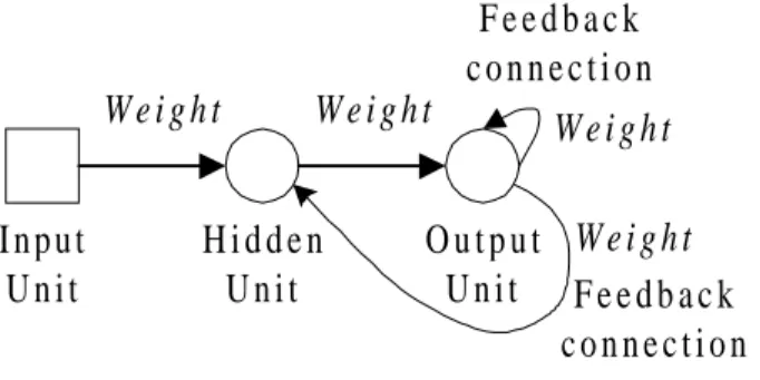
handle temporal information and model systems with internal state. Figure 2.6 is

an example of how a recurrent network could look like.

Figure 2.6: A recurrent network.

Russell and Norvig argue, when network architecture is chosen, one has to be very

careful so the network will be the “right one”, e.g. if the chosen network is too small

(i.e. few layers or too few hidden units) then it will be incapable of representing the

desired function. If the network is to big (i.e. too many hidden units) then it will be

able to memorize all the examples by forming a lookup table, but will not generalize

well to inputs that have not been seen before.

2.2.2

How do the ANNs work

Each of the input neurons holds a specific component of the input pattern and

normally does not process it, but simply sends it directly to all the connected neurons.

However, before their output can reach the following neurons, it is modified by the

weight on the connection. All the neurons of the second layer then receive modified

input values and process them. Afterwards these neurons send their outputs to

succeeding neurons of the next layer. This procedure is repeated till the neurons of the

output layer finally produce an output.

2.2.3

Learning in ANNs

Once a network has been structured for a particular application, that network is ready

to be trained. To start this process the initial weights are chosen randomly, then the

training, or learning, begins. There are three main classes of learning in ANNs.

•

Supervised: In supervised learning, learning occurs when the system directly

compares the network output with a known correct or desired answer in the

training process. Many iterations through the training data may be required before

the net begins to work properly.

•

Unsupervised: In unsupervised learning the weights of the net can be modified

without specifying the desired output for any input data. The net just looks at the

data it is presented with, finds out about some of the properties of the data set and

learns to reflect these properties in its output. What exactly these properties are,

I n p u t

U n i t

H i d d e n

U n i t

O u t p u t

U n i t

W e i g h t

W e i g h t

F e e d b a c k

c o n n e c t i o n

W e i g h t

F e e d b a c k

c o n n e c t i o n

W e i g h t

and learning method. Usually, the net learns some compressed representation of

the data, c.f. [Sar97].

•

Reinforcement: The network receives a reward or penalty depending on how it

performed a certain task. If supervised training is “learning with a teacher”,

reinforcement training is “learning with a critic” [Tay95]. The major difference

between supervised learning and reinforcement learning is that supervised

learning gets/gives correct output in every time step, but reinforcement learning

only occasionally “good” or “bad”.

One of the most significant attributes of a neural network is its ability to learn by

interacting with its environment. As Hassoun [Has95] describes, learning in a neural

network is normally accomplished through an adaptive procedure, known as a

learning rule or algorithm, which defines how the weights of the neural network are

adjusted to improve the performance of the network. Therefore they need to explore.

It is interesting to note that supervised learning systems do not have this problem.

They are told what output should be produced at every step in time. But reinforcement

learning systems have a greater “responsibility” in that they are not told explicitly

what output should be produced. Therefore they must make more independent

decisions at intermediate stages.

2.2.4

Why use ANNs ?

According to Taylor [Tay95], there are many problems in industry and business that

are beyond the scope of the present generation of computers. They run into trouble if

data is incomplete or contains errors or if it is not clear how a problem should be

solved. ANNs are already handling these kinds of complex tasks in areas such as

machine vision, robotics, and cost analysis, and even share price and currency

prediction. ANNs can learn if they are presented with a range of examples, deduce

their own rules for solving problems, and produce valid information from noisy data.

As Fausett [Fau94] describes, one of the greatest advantages of ANNs is the ability to

learn from examples, which is a fundamental characteristic of intelligence. Most

software is programmed to perform fixed tasks. The ANNs are taught to do some

desired tasks and not given a step by step procedure to perform the tasks, i.e. ANNs

can learn from training by adjusting the weight of the connections to perform certain

tasks. To have learning abilities distinguishes ANN software from other software.

As described by Taylor, it is clear that in actual application studies ANNs acting in

stand-alone fashion are not generally flexible or powerful enough, at present, to deal

with more than two or three tasks. Important issues are therefore which tasks should

be left for the ANNs to deal with and which should be formally dealt with by an

alternative mechanism.

2.3

Related work

As described by Saunders and Pollack [Sau96], there are lots of projects that have

been done concerning multiple robots, autonomous agents and cooperation. Many are

currently being done, but there are not so many that involve study of communication

schemes.

2.3.1

Work related to communication schemes and cooperation

Little work has been done that describes how to let robots cooperate just by using

simple communication schemes. However, Saunders and Pollack [Sau96], describe

how robots can cooperate by using simple communication schemes. In this study

Saunders and Pollack explore a method which communication can evolve. The agents

are modeled as connectionist networks. Each agent is supplied with a number of

communications channels implemented by the addition of both input and output units

for each channel. An agent does not receive input from other individuals, rather the

agent’s inputs reflects the summation of all the other agents’ output signals along the

channel. Saunders and Pollack focused on how a set of agents can evolve a

communication scheme to solve a modified “Tracker Task” (The Tracker Task is

described by [Sau96] and figure 2.7). The modified “Tracker Task” is to let simulated

agents learn to find “food” (which is all concentrated in a small area in the center of

the environment) and when the “food” is found the agents communicate, so the other

agents can come to the area. They used GNARL [Sau96], an algorithm based on

evolutionary programming that induces recurrent neural networks, but there are no

detailed descriptions of the algorithm included in the study. Figure 2.8 show how the

network semantic is in Saunders and Pollack study.

Figure 2.7: FSA hand-crafted for the Tracker task. The large arrow

indicates the initial state. This simple system implements the strategy

“move forward if there is food in front of you, otherwise turn right four

times, looking for food. If food is found while turning, pursue it,

otherwise, move forward one step and repeat.” From [Sau96]

F o o d / M o v e

F o o d / M o v e

N o F o o d / R i g h t

F o o d / M o v e

F o o d / M o v e

F o o d / M o v e

N o F o o d / M o v e

N o F o o d / R i g h t

N o F o o d / R i g h t

N o F o o d / R i g h t

Figure 2.8: The semantic of the I/O units for evolving communication.

The “food/nofood” inputs are from the Tracker task. The “Follow FSA”

node represent one particular strategy found by GNARL (shown in figure

2.7). The additional nodes, give the agent the ability to perceive, generate,

and follow signals. From [Sau96]

The result to this study was that the GNARL algorithm is capable of evolving a

communication scheme, which allows the agents to perform their task. One of the

purposes with this work was to open the door to the study of evolving continuous

communication schemes.

2.3.2

Work related to multiple robots

Research about problems with multiple robots has been done at The University of

Michigan by Huber and Kenny [Hub94]. This research presents a number of issues

that arise when making the transfer from single robot to multiple robots, or simulated

robot to working with robot situated in a real world. This research describes also how

two real robots could work together when pushing obstacles.

Huber and Kenny briefly talk about many of the issues that arise when working with

multiple robots, such as those that deal with communication, organization,

cooperation strategies, etc. They also point out where more in-depth discussions can

be found.

The main purpose of this research was to give better understanding of problems that

can arise when working with multiple robots and suggestions how to eliminate or

minimize these problems.

Fully connected

h i d d e n u n i t s ( k )

F o l l o w F S A

F o l l o w g r a d i e n t

_{1 2 ... n}

O u t p u t s i g n a l

_{1 2 ... n}

1 2 ... n

I n p u t s i g n a l

F o o d

N o F o o d

3

The simulator

The Khepera Simulator is a public domain software package developed by Olivier

Michel during the preparation of his Ph.D. [Mic96]. It will be used in all the

experiments that will be done in this study.

The simulator runs on most Unix-compatible systems and features a nice X11

graphical interface. It allows you to write your own controller for the mobile robot

Khepera using C or C++ and to test them in a simulated environment. It can also drive

the real robot using the same control algorithm. The Khepera Simulator is mainly

intended for the study of autonomous agents.

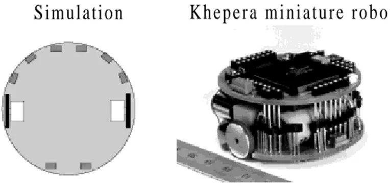
Figure 3.1: The simulated Khepera robot and the real Khepera miniature

robot.

The real Khepera miniature is a small mobile robot (55 mm in diameter). It is

equipped with two motors connected to two wheels (one on each side) and 8 pairs of

sensors placed around with its body (6 in the front, 2 at the back), see figure 3.1.

The screen of the Khepera Simulator is divided into two parts as shown in figure 3.2:

Figure 3.2: Screen shot of the simulator. From [Mic96]

•

The world (on the left): In this part one can observe the behaviour of the robot in

its environment.

•

The robot (on the right): In this part one can observe what is going inside the

robot, i.e. the activity of sensors and motors. This part can also be used for

displaying all the information that is relevant for the simulator, i.e. variables,

results, graphs, neural network, etc.

3.1

Description of the world

Various worlds are available for the simulator. It is also possible to create a new one

or edit an old, to make new worlds. The real dimensions of this simulated

environment, comparing to the real robot Khepera, are 1m × 1m (i.e. all the area

available in the world part).

In this study the worlds in figure 3.3 will be used for testing (mainly empty.world and

home.world).

Figure 3.3: Three different simulated worlds. From [Mic96]

3.2

Description of the robot

The simulated Khepera robot is equipped with 8 distance sensors (small rectangles)

and 8 light sensors (small triangles) placed around with its body. There is also a motor

on each side of the robot. See figure 3.4.

Figure 3.4: Simulated Khepera robot. From [Mic96]

e m p t y . w o r l d

h o m e . w o r l d

m a z e . w o r l d

S e n s o r 1 S e n s o r 6 S e n s o r 2 S e n s o r 3 S e n s o r 4 S e n s o r 5 S e n s o r 8 S e n s o r 7

F r o n t

R e a r

L e f t M o t o r R i g h t M o t o r W h e e l W h e e l

3.2.1

Distance sensors

Each distance sensor returns a value ranging between 0 and 1023. 0 means that no

object is perceived while 1023 means that an object is almost touching the sensor (if

not touching it).

Each sensor scans a set of 15 points in front of it. See figure 3.5. If an obstacle is

present under a given point, the value associated to that point is added to a sum. This

sum is the return value of the sensor. Noise is added to this sum before it is returned

as the response value of the distance sensor. A random noise of ±10% is added to the

distance value output.

Figure 3.5: Sensor values and position of the points (taken from the source

code).

3.2.2

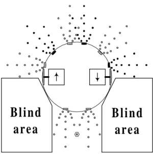
Blind areas

A robot that moves backward is very likely to collide with obstacles and get stuck.

The blind areas are due to of the position of the sensors and/or number of sensors. See

figure 3.6.

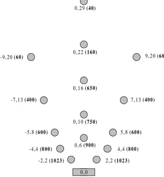
mm from sensor to right/left (+/-), mm from sensor (value)

- 2 , 2 (1 0 2 3 ) 2 , 2 ( 1 0 2 3 ) 4 , 4 ( 8 0 0 ) - 4 , 4 (8 0 0 ) - 5 , 8 ( 6 0 0 ) 5 , 8 ( 6 0 0 ) - 7 , 1 3 ( 4 0 0 ) 7 , 1 3 ( 4 0 0 ) 9 , 2 0 ( 6 0 ) - 9 , 2 0 ( 6 0 ) 0 , 6 ( 9 0 0 ) 0 , 1 0 ( 7 5 0 ) 0 , 1 6 ( 6 5 0 ) 0 , 2 2 ( 1 6 0 ) 0 , 2 9 ( 4 0 ) 0 , 0

Figure 3.6: The blind areas.

3.2.3

Motors

The motor drive a wheel on each side of the “body”, see figure 3.4. By varying the

speeds of the motors, the robot can go forwards, backwards or turn in any direction.

Each motor can take a speed value ranging between –10 and +10.

A random noise of ±10% is added to the motor speed and a random noise of ±5% is

added to the direction resulting from the difference of the speeds of the motors.

B l i n d

area

B l i n d

area

4

Problem description

In this project a multi-agent neural controller will be implemented for the Khepera

Simulator. The simulator, environment and the robot that will be used in this study,

have been described in chapter 3.

The simulator is supposed to simulate the robot behaviour and to see if it is possible to

get cooperation using simple communication schemes, as described in section 1.1. In

other words, it will be investigated how it would be possible to train multiple mobile

robots to stay close to each other while avoiding collisions with each other and other

obstacles.

When the robots come into contact with each other they are supposed to coordinate

their actions so they will not collide with each other or obstacles as seen in figure

4.1-4.4. They are also supposed to stay in contact to each other all the time after they have

start coordinating their actions.

Figure 4.1: Two robots get in contact. Robot-B uses the outputs it gets

from Robot-A to stay in contact and not being to close to it, i.e.

Robot-A only does obstacle avoidance.

Figure 4.1 and 4.2 show what it could look like when two robots come into contact

with each other and there is enough space (i.e. no obstacles in the way) to let them

move just according to the output the get from each other.

Figure 4.3: Two robots get in contact and both use the outputs they get

from each other to stay in contact and not being to close to each other.

Figure 4.4: Two robots get in contact and both use the outputs they get

from each other to stay in contact and not being to close to each other.

Figure 4.3 and 4.4 show how it could look like if there was an obstacle in their way.

In figure 4.3 and 4.4 both robots use the outputs they get from each other to

coordinate their actions. On the other hand in figure 4.4 Robot-A works as master and

Robot-B as slave, that means that Robot-B only follows Robot-A and has to take care

of staying in contact. The robots could hand over and take over the master role when

there were a situation like in figure 4.4. However, in this study, it will only be tested

to use the same master and slave all the time, so it will not be studied how to hand

over and take over the master role.

In this study the Khepera simulator will be used with two simulated robots. The

simulator adds a random noise to the data that the robots perceive with the sensors to

make it more realistic. All the work will be done in a 2-dimensional world.

4.1

Activities which the robots have to accomplish

•

Controlling the motion of its wheels.

•

They should never come into collision with obstacles or other robots.

•

They should work like autonomous robots, i.e. make decisions on their own,

guided by the information they get from their input units.

4.2

A number of factors that will be studied

•

How to cooperate using simple communication schemes.

•

How to distinguish robots from other obstacles.

•

How to let the robots not be closer to each other than a certain distance.

•

Obstacles may block the robot’s path.

4.3

A number of factors that will not be studied

•

How to operate moveable parts.

•

How to work in a 3-dimensional world or real world.

•

How to hand over and take over the master role.

•

How to add more robots to the simulator.

•

The robots may run out of power.

•

The robots may be working in noisy environment.

•

Which type of communication to use in different environments.

•

Unpredictable events may leave little time for responding.

4.4

Expected results

The aim of this study is to find out if and how cooperation between autonomous

mobile robots can work using only simple communication schemes in ANNs by using

the Khepera Simulator.

How can it be determined when a solution is found? It will be when the robots can

stay in contact to each other all the time after they have started coordinated their

actions, without colliding with each other and other obstacles.

One of the many problems in this study is to choose the right ANN and the right

learning algorithm to solve the problem. This will be discussed in chapter 5.

5

Method

In this chapter the approach is described.

5.1

Choice of ANN architecture

As Sarle [Sar97] describes, ANNs cannot do anything that cannot be done using

traditional computing techniques, but they can do things that would otherwise be very

difficult. In this study feed-forward networks will be used, in particular for that they

are widely used and well understand, and due to their simplicity.

As described in [Glo95], recurrent networks are able to store information, and

therefore they are particularly suitable for forecasting events, e.g. in this study to

predict/detect motion. They have also been used with considerable success for

predicting several types of time series, as described in [Glo95]. However, while

recurrent neural networks have many desirable features, there are practical problems

in developing effective training algorithms for them. Russell and Norvig [Rus95]

point out that recurrent networks can become unstable, or exhibit chaotic behaviour.

When given some input values, it can take a long time to compute a stable output and

learning is therefore made more difficult. Recurrent networks also often require some

quite advanced mathematical methods. This is one of the many reasons recurrent

networks are not used in this study. However, recurrent networks can implement more

complex agent designs than feed-forward.

It will be evaluated which type of feed-forward network is most appropriate for each

experiment.

5.2

Choice of learning method

There are many learning methods for ANNs. According to [Sar97], nobody knows

exactly how many and new ones are invented all the time.

As described in [Har97], there are many situations where we do not know the correct

answers that supervised learning requires, e.g. in this study, the input would be the set

of all sensor readings at a given time. The output would be the values the robot

motors should get according to the sensor input, but the “right” output is not known.

The ANNs can not learn to control the robot in this project as wished by using simple

supervised learning unless there was a set of known “answers”. Therefore

reinforcement learning (described in section 5.2.1) will be used in this study.

Russell and Norvig [Rus95] argue that one of the most common algorithms for

training multilayer feedforward networks is backpropagation learning algorithm.

Backpropagation algorithm (described in section 5.2.2) will be used in this study with

help from the reinforcement learning.

5.2.1

Reinforcement Learning

Reinforcement learning has often been used in cooperative robotics and has shown

good results, according to Fukunaga [Fuk96]. This is one of the many reasons why

reinforcement learning will be used in this study.

Fukunaga argues that reinforcement learning is especially attractive for problems in

robotics, as it is often found that the robot's creators do not have enough knowledge to

program or teach the robot everything it needs to know. Reinforcement learning

allows the programmer to set the robot a goal, tell it whatever can be easily taught,

and then allow it discover the details on its own.

5.2.1.1

How reinforcement learning works

As described in [Fuk96], reinforcement learning is a kind of machine learning, in

which an agent is given a task to perform, and it learns how to do it by a process of

trial and error. The agent makes an action depending on what it perceives from the

environment. Depending on that action a reward or penalty is sent (reinforcement

signal) which will indicate whether this action was “good” or “bad”, i.e. the agent will

get into a new state and will get reinforcement signal depending on the new state in

the environment. The signal (reinforcement signal) will be used in the learning

function which will send a learning signal (to optimize the weights) to the agent in

such a way as to maximize the good actions while minimizing the bad. This process is

shown in figure 5.1. The ultimate goal of the agent is to learn a strategy for selecting

actions or policy such that the expected sum of rewards is maximized.

Figure 5.1: The system and the environment. From [Zie96]

5.2.1.2

Possible rewards and penalties for the robot

•

The robot will get reward for moving a wheel. More reward for moving forwards

than for moving backwards. The reason for the robot will get more reward for

moving forward than moving backwards is because it is more likely to get stuck if

it moves backwards.

•

The robot will get penalty for stopping wheel, i.e. motor value = 0.

•

The robot will get penalty for being too close to the other robot

•

The robot will get penalty for being too far from the other robot, i.e. being out of

“signal” range.

•

The robot will get reward for having the other robot in “signal” range, and not

being too close to it.

•

The robot will get penalty for being to close to obstacle and the penalty will

increase if the robot moves closer to the obstacle.

Controller

( A g e n t )

E n v i r o n m e n t

R e i n f o r c e m e n t

signal

Learning signal

p e r c e p t s

actions

•

The robot will get reward for being away from obstacles, i.e. the robot should try

to avoid obstacles.

The “signal” detector/sender will be described in chapter 6.

5.2.2

Backpropagation learning algorithm

As described in [Has95], backpropagation is one of the most frequently used learning

rules in many applications of ANNs. In fact, the development of backpropagation is

one of the main reasons for the renewed interest in ANNs. Backpropagation provides

a computationally efficient method for changing the weights in a feedforward

network, with differentiable activation function units. Backpropagation trained

multilayer ANNs have been applied successfully to solve some difficult and diverse

problems, such as nonlinear system, and pattern classification, etc.

Backpropagation learning is a gradient descent search algorithm that may suffer from

slow convergence to local optimal solution, and there is no guarantee that it will find a

global solution, according to Russell and Norvig [Rus95].

“Backpropagation provides a way of dividing the calculation of the

gradient among the units, so the change in each weight can be calculated

by the unit to which the weight is attached, using only local information.”

[Rus95, page 582]

When working with backpropagation learning one is trying to find the difference

between the output value and the target value (an error), and then divide it among the

contributing weights. In this research there are no known target values, so this needs

another solution. The intention with using the reinforcement signal is to find the

“error”, so the “correct” weights can be found for the network. It will then be tried to

give reward/penalty in some sensible way depending on the experiment.

err = maximum reward – actual reward/penalty

(EQ 5.1)

err is the error value.

maximum reward is the highest possible reward that the robot can get.

actual reward/penalty is the actual reward/penalty, which is (actual reward – actual

penalty).

Then the weights would be updated according to:

W

jinew

= W

jiold

+

∆W

ji

(EQ 5.2)

where

∆W

ji

=

α * a

j

*

∆

i

(EQ 5.3)

with

∆

i

= err * g’(in

i

)

(EQ 5.4)

and

W

kjnew

= W

kjold

+

∆W

kj

(EQ 5.5)

where

∆W

kj

=

α * I

k

*

∆

j

(EQ 5.6)

∆

j

= g’(in

j

)*

∑

i

(W

jiold

*

∆

j

)

(EQ 5.7)

To get more understanding over the values (I

k

, W

kj

, a

j

and W

ji

) see figure 5.2.

Figure 5.2: A feed-forward network

W

jinew

is the new weight between hidden unit j to output unit i.

W

jiold

is the old weight between hidden unit j to output unit i.

∆W

ji

is the change in weights between hidden unit j to output unit i.

α is the learning rate that determines the size of the steps that will be taken, when

learning takes places (small positive value).

a

j

is activation value of unit j, (it can also be output from another unit).

g’(in

i

) is the derivative of the activation function of the output unit.

W

kjnew

is the new weight between input unit k to hidden unit j.

W

kjold

is the old weight between input unit k to hidden unit j.

∆W

kj

is the change in weights between input unit k to hidden unit j.

I

k

is the input value that the input unit k gets.

g’(in

j

) is the derivative of the activation function of the hidden unit.

5.2.3

How to find the “correct” weights

According to [Fuk96], finding the correct values for the weights that lead to a desired

cooperative behavior can be a difficult and time-consuming task for a human

designer. Therefore, it is highly desirable for multiple-robot systems to be able to

learn to find the “correct” weights in order to optimize their task performance, and to

adapt to changes in the environment.

In “normal” ANN learning there is a credit assignment problem, i.e. one does not

know which weights are not “correct” and therefore “did wrong”. When working with

multiple-robot systems one has a robot assignment problem, i.e. one does not know

which robot did wrong (e.g. if they collide).

In this study each individual weight get a random strength (weight) between 0-1.0 in

the beginning. The rewards/penalties will be used to adjust the weights and hopefully

find the “correct” weight at the end.

Input Layer

H i d d e n L a y e r

O u t p u t L a y e r

W e i g h t s

W e i g h t s

I

k

W

_k,j

a

j

W

_j,i

O

_i

6

Changes made to the simulator

Few changes had too be done to the simulator so it was possible to do the desired

tasks describe in chapter 4 and to make it easier to observe two robots at the same

time. These changes are described in this chapter.

6.1

Changes made to the robot

One change was made to the robot in this study.

A “signal” detector/sender was added to the robot. This “signal” detector/sender is

very simple, it can only sense the distance to the other robot and it has a maximum

distance range. See figure 6.1. The robot sends a signal from it, and the other robot

gets a signal of a different strength depending on how close it is to the robot, i.e. the

“signal” detector gets a value that tells the robot how far away it is to the other robot.

Figure 6.1: The “signal” detector/sender of the robot.

This was done because the distance sensors are not powerful enough to let the robots

have longer minimum distance between each other than from other obstacles. The

robots get one input that indicate the distance between the robots, but not where the

robot is. The value of the distance between the robots will get random noise of ±5%.

6.2

Changes made in the robot part of the screen

Few changes were made in the robot part.

All changes are marked in figure 6.2 with a number in a star. The changes made to the

original code are shown in appendices A-F.

M a x i m u m s i g n a l r a n g e

_{The other robots should}

Figure 6.2: The robot part of the Khepera Simulator. (This ANN is the

same as will be used in experiment 1.)

6.2.1

Changes that can be seen

1.

An extra robot was added to the robot part, so now it is possible to see activity in

both robots at the same time.

2.

An Init-button was added. It is used to initialize the multirobots.

3.

An extra Step-Button was added. It is for letting the multirobots take one step at a

time.

4.

An extra Run-Button was added. It is for letting the robots move undisturbed until

the button is pressed again.

5.

Both the ANNs are now shown at the same time, instead of only one at the time.

So it is possible to see the neurons activities of both ANNs at the same time.

6.

In the original simulator you can only see maximum 17 input neurons on the

1

2

3

4

5

6

8

7

9

7.

Here will a message be written which will say if the robots are in the right place,

too far away from each other or to close to each other.

6.2.2

Changes that can not be seen

8.

Now the ANNs get random weight between 0 – 1.0 when you load a new one (by

pressing the new-button).

9.

Not all the neurons in the network will use the same activation function, e.g. in

experiment 1 the output neurons will have a different activation function from the

other neurons. See section 7.1.2 (experiment 1) for details.

7

Implementation

In this chapter 4 different experiments will be described.

7.1

Experiment 1

The robots will both be using the same type of network in this experiment. The ANNs

get random weights in the beginning, only one robot (Robot-1) has the ability to learn

and can change the weights in its network. The other robot (Robot-2) will only use the

random weights it gets in the beginning and can not change its network weights. The

learning will only concern that the robot (Robot-1) will have to avoid obstacles and

move all the time. In this experiment the different behaviour of the robots will be

studied.

7.1.1

The aim

The aim of this experiment is to show that it is possible to train a robot to avoid

obstacles in the Khepera simulator. Then in experiment 2, communication will be

added. Experiment 1 is done to get more understanding of how the robot works,

before more factors are studied at the same time.

7.1.2

The network

The feed-forward network in figure 7.1 will be used in this experiment which will

result in a purely reactive agent. Sensor 1 is connected to input unit 1, sensor 2 to

input unit 2, etc.

Figure 7.1: Feed-forward net for experiment 1.

Figure 7.2 illustrate how the network looks like in the robot.

This network is not fully connected. The main reason for that is because after some

study it was noticed that the sensors 1-3 should affect the right-motor (slow down the

motor) and the sensors 4-6 should affect the left-motor. The output units get a value

from 0 – 1, where 0 means the speed 10 and 1 means the speed -10, so when the units

I n p u t L a y e r

H i d d e n L a y e r

O u t p u t L a y e r

S e n s o r 1

S e n s o r 3

S e n s o r 5

S e n s o r 7

S e n s o r 2

S e n s o r 4

S e n s o r 6

S e n s o r 8

L e f t - M o t o r

R i g h t - M o t o r

W e i g h t s

W e i g h t s

It is not usual to connect only one input unit to a hidden unit, but in this experiment

sensors 7 and 8 are connected to a hidden unit that has a negative activation function.

So when they are activated the motor should get higher speed (this is described in

section 7.1.3).

Figure 7.2: The ANN in the simulated robots in experiment 1.

7.1.3

The values for the learning function

The activation function was simply x

2

and the derivation of the activation function

2x. For all units excepts the two units in the hidden layer that were connected to the

sensors in the back.

The two units in the hidden layer that were connected to the sensors in the back were

not using the same activation function as the others units, they had the activation

function -x

2

. This was done because when the robot had an obstacle in the back the

robot back into it and got stuck. So by changing the activation function for these two

units this problem was solved. Instead of having different activation functions it could

be possible to let the network learn negative weights. The main reason for that this

was not done in this experiment was that, it was decided in the beginning that the

weights should be between 0-1. So the first solution to this problem was to let the

network have different activation functions.

•

The robot got 10 in reward for moving a wheel forward and 5 for moving

backwards.

•

The robot got 20 in penalty for stopping wheel, i.e. motor value = 0.

•

The robot got (3-34) in penalty for having obstacles too close to sensor in front of

the robot and the penalty increased when the robot moved closer to the obstacles.

•

The robot got (6-68) in penalty for having obstacles too close to sensor in back of

the robot and the penalty increased when the robot moved closer to the obstacles.

•

The robot got penalty for being to close to the other robot, the same as for being to

close to obstacles.

Front

•

The robot got (2 or 3) in reward for being away from obstacles, i.e. 3 for sensor in

front and 2 for the sensor in back.

Modifications were made to the equation (EQ 5.1).

err = – penalty

(EQ 7.1)

if the reward were higher than penalty and the learning rate

α = 0.05 but else

err = (maximum reward - (reward - penalty)) - reward

(EQ 7.2)

and the learning rate

α = 0.01

The maximum reward in this experiment is 42 and maximum penalty is 380.

The equation 7.1 can get error value from –39 to 0 and the equation 7.2 can get error

value from 0 to 422.

The error equation and the values for reward and penalty were chosen through

experiments.

7.1.4

Result from experiment 1

This seemed to work, as it should do in the beginning, the robot moved all the time

and “never” got stuck, i.e. when it got stuck it managed to get it loose by it self. The

robot was learning all the time and the weights were always changing, so after about

20.000 - 200.000 steps the robot suddenly got stuck and could not move at all. So the

program needed a little change, the changes that where made was that the learning

rate of the robot was decreased once every 1000 step with the equation 7.3.

α = α / (step / 1000)

(EQ 7.3)

After this change the robot was able to move over 1.000.000 steps without getting

stuck. The robot moves about 7000 steps in one minute, using Linux on Pentium 133,

so it takes about 2 hours and 23 minutes to do 1.000.000 steps. It took the robot about

5.000 – 30.000 steps to set the weights right, so it managed to stay away from the

walls and move all the time.

It is possible to print out the values of the network weights in the Khepera Simulator.

The network for Robot-1 after 0 steps, 20.000 steps and after 1.000.000 steps is

shown in Appendix H.

As suspected before testing experiment 1, Robot-2 did not perform well, this was

because it only got random weights. But sometimes the robot managed stay away

from obstacles, i.e. when it got random weights that where near desirable values.

Robot-2 never managed to move more than 2000-8000 steps without getting stuck and

when it got stuck it had no possibility to get loose.

7.1.5

How experiment 1 works

If the robot moves towards a wall and the sensors in front are not sensitive enough the

robot fixes its weights so it can get from the wall. In the beginning the robot stops in

front of the wall (see figure 7.3), but after little while the sensors will be more

sensitive and the robot should move from the wall by turning around and heading

forward. This is shown in figure 7.4.

Figure 7.3: Simulated robot stuck in front of a wall.

This situation will give the robot 30 in reward and 60 in penalty, so the error value is

62, i.e. (42-(30-80))-30 = 62. All the weights will then increase and the connection

that has the highest input (1023) will get the highest changes in weights so after a

little while the robot will turn around and move from the wall, i.e. the sensors in front

will be more sensitive than before.

The source code for experiment 1 is shown in Appendix G.

Figure 7.4: Simulated robot stuck, moves from the wall and heads

forward.

7.1.6

Learning in different worlds

When the robot learned in empty.world the sensors in the back or at one side of

the robot were not used so often. So maybe after 20.000 steps the robot came

into situations where it had to use these sensors, then the sensors were not

sensitive enough and the robot got stuck. One situation where this can happen is

where the robot would be moving in big circles, i.e. if the weights to one motor

were smaller than to the other.

When the robot learned in home.world all the sensors were activated often so

the robot managed to set its weights “right”. After learning in the home.world

the robot could move in empty.world without getting stuck. So all the learning

was done in home.world.

1 0 2 3 1 0 2 3

1 7 6

2 1 4

3

1

5

1 0

1 0

4

- 1 0

- 1 0

2

2

1 0

1 0

1 0 2 3 1 0 2 3

2

0

1 1 7

1 9 7

7 1 3

-8

4 7 5

2 1

0

2

5

3

6

3

5

2 5

5

2

0

1

3

5

7.2

Experiment 2

The ANNs get random weights in the beginning, only one robot (Robot-1) has the

ability to learn and can change the weights in its network. The other robot (Robot-2)

will only use the random weights it gets in the beginning and can not change its

network weights. The learning will concern training Robot-1 to stay close to Robot-2

while avoiding collisions with other obstacles, and when Robot-1 has once contact

with Robot-2 it is supposed to stay in contact all the time.

After a little time it was obvious that it was not possible to let the robots distinguish

robots from other obstacles because of the low range of the distance sensors (i.e. only

29 mm), so this required for another solution. The change that was made was to add

the “signal” detector/sender (with a range of 25 cm, in this experiment) on the robots

so they can detect how far from each other they are (with random noise of ±5%). This

gave opportunity for another task that the robot could try to achieve. The robots could

try to be not far from each other than a certain distance (20 cm) and to stay within a

certain distance from each other (5 cm), i.e. they could not be too close to each other

and not too far away from each other. The signal could also include which robot is

sending it, when working with more than two robots.

7.2.1

The aim

The aim of this experiment is to show how it works to train robots to stay close to

each other, by communicating, while avoiding collisions with other obstacles. This is

the main purpose of this study and therefore it is important to show how the robots

can solve this by communicating. The robots send their outputs all the time to the

other robot and when they are in signal range, they also get the signal value.

7.2.2

The network

The feed-forward network in figure 7.5 was used in this experiment, which result in

purely reactive agent. Sensor 1 is connected to input neuron 1, sensor 2 to input

neuron2, etc. The Signal Sender is the “signal” the other robot detects for knowing the

distance between the robots.

Figure 7.5: Feed-forward net for Robot-1 in experiment 2.

Figure 7.6 shows how the robots networks are connected together, when the robots

are communicating.

I n p u t L a y e r

H i d d e n L a y e r

O u t p u t L a y e r

S e n s o r 1

S e n s o r 3

S e n s o r 5

S e n s o r 7

S e n s o r 2

S e n s o r 4

S e n s o r 6

S e n s o r 8

Left-Motor

R i g h t - M o t o r

W e i g h t s

W e i g h t s

Signal

F r o m

Robot-2

Robot-2

Left

M o t o r

Robot-2

R i g h t

M o t o r

S i g n a l S e n d e r

Figure 7.6: The robots’ feed-forward nets connected.

7.2.3

Result for experiment 2

After some studying it was clear that this experiment could not be solved by using the

network in figure 7.5. The robot only got distance to the other robot and could

therefore be anywhere in the radius around the robot. The only way Robot-1 could

learn to stay close to Robot-2 in this experiment was if they were heading in the same

direction and Robot-1 would do “exactly” the same things that Robot-2. But when

Robot-1 would detect an obstacle it would have to avoid it and therfore it could lose

conntact with Robot-2, i.e. if it would not know “exactly” where Robot-2 was. So to

solve this problem it is necessary to develop (program) an algorithm that can calculate

the exact position of the other robot or/and choose some other network. The algorithm

would have to use the input that Robot-1 gets from Robot-2, and its own output values

to calculate the position. The algorithm would have to use at least two steps to

calculate the position. This will be tested in experiment 3.

7.3

Experiment 3

The ANN for Robot-1 gets random weights in the beginning, and Robot-1 has the

ability to learn so it can change the weights in its network. Robot-2 will be using the

weights taken from experiment 1 (shown in Appendix H), so it will only be doing

simple obstacle avoidance. Robot-1 is supposed to learn to follow Robot-2 while

avoiding colliding with it and other obstacles. In this experiment an algorithm will be

designed to make inputs for Robot-1 from the outputs that Robot-2 sends. The

algorithm will calculate the relative position of the other robot. Then the algorithm

will make inputs for the robot, which the robot will have to learn how to use.

The reason for why position works better than distance is that if the robot know that

the other robot is on the right side of it, it should turn right (to the robot) instead of

left (away from the robot). With distance only the robot could never determine if the

other robot is on the left or right.

The robots will communicate all the time while Robot-1 is learning. When learning

stops communication will only take places when they are in “signal” range to each

other, so the robot should never go out of “signal” range.

7.3.1

The aim

The aim of this experiment is to show that it is possible to let the robots cooperate by

using the solution from experiment 2, i.e. by using position instead of distance. The

robot will still be an autonomous robot by learning how to use the inputs given from

the algorithm.

7.3.2

The network

Figure 7.7: The robots’ feed-forward nets connected with the algorithm.

The network for Robot-1 is almost the same as was used in experiment 1, the only

different is the extra inputs that the algorithm produced. The inputs that the algorithm

produced were not fully connected as it was noticed that some of the inputs should

only affect one of the motors, this was done to speed up the learning and to make it

easier. In figure 7.7 the network of the robots is shown when connected together.

7.3.3

The algorithm

The algorithm used the information given from the simulator i.e. the position of the

robots and which direction Robot-1 where heading. Then it used the “signal” from the

robot that indicated how far away the robots are.

By using the position of the robots it was possible to calculate the angle to Robot-2

from this point see (EQ 7.4). Then it was necessary to use the direction of Robot-1 to

calculate the relative angle to Robot-2 see (EQ 7.5).

Angle = arcsin((1/HowFarAway)*(abs(YRobot1-YRobot2))

(EQ 7.4)

Angle is the angle between the robots, if Robot-1 was heading up (in the simulator).

HowFarAway is the distance between the robots.

YRobot1 is the Y-coordinate in the simulator for Robot1.

YRobot2 is the Y-coordinate in the simulator for Robot2.

Angle = (Angle - (Alpha –

π/2))

(EQ 7.5)

Angle is the relative angle between the robots.

Alpha is the direction of Robot-1 in the simulator.