M
ÄLARDALENU
NIVERSITYS
CHOOL OFI
NNOVATION,
D
ESIGN ANDE
NGINEERINGV
ÄSTERÅS,
S
WEDENExamensarbete för kandidatexamen i datavetenskap | DVA331
C
ONTACT
-
FREE
C
OGNITIVE
L
OAD
C
LASSIFICATION BASED ON
P
SYCHO
-P
HYSIOLOGICAL
P
ARAMETERS
Johannes Sörman
Jsn16009@student.mdh.se
Rikard Gestlöf
Rgf16001@student.mdh.se
Examiner:
Mobyen Ahmed
Mälardalen University, Västerås, Sweden
Supervisor: Hamidur Rahman
Mälardalen University, Västerås, Sweden
Abstract
Cognitive load (CL) is a concept that describes the relationship between the cognitive demands from a task and the environment the task is taking place in, which influences the user’s cognitive resources. High cognitive load leads to higher chance of a mistake while a user is performing a task. CL has great impact on driving performance, although the effect of CL is task dependent. It has been proven that CL selectively impairs non-automized aspects of driving performance while automized driving tasks are unaffected. The most common way of measuring CL is electroencephalography (EEG), which might be a problem in some situations since its contact-based and must be connected to the head of the test subject. Contact-based ways of measuring different physiological parameters can be a problem since they might affect the results of the research. Since the wirings sometimes might be loose and that the test subject moves etc. However, the biggest concern with contact-based systems is that they are hard to involve practically. The reason for this is simply that a user cannot relax, and that the sensors attached to the test subjects can affect them to not provide normal results. The goal of the research is to test the performance of data gathered with a contact-free camera-based system compared to a contact-based shimmer GSR+ system in detecting cognitive load. Both data collection approaches will extract the heart rate (HR) and interbeat interval (IBI) while test subjects perform different tasks during a controlled experiment. Based on the gathered IBI, 13 different heart rate variability (HRV) features will be extracted to determine different levels of cognitive load. In order to determine which system that is better at measuring different levels of CL, three major stress level phases were used in a controlled experiment. These three stress level phases were the reference point for low CL where test subjects sat normal (S0), normal CL where the test subjects performed easy puzzles and drove normally in a video game (S1) and high CL where the test subjects completed hard puzzles and drove on the hardest course of a video game while answering math questions (S2). To classify the extracted HRV features from the data into the three different levels of CL two different machine learning (ML) algorithms, support vector machine (SVM) and k-nearest-neighbor (KNN) were implemented. Both binary and multiclass feature matrixes were created with all combinations between the different stress levels of the collected data. In order to get the best classification accuracy with the ML algorithms, different optimizations such as kernelfunctions were chosen for the different feature matrixes. The results of this research proved that the ML algorithms achieved a higher classification accuracy for the data collected with the contact-free system than the shimmer sense system. The highest mean classification accuracy was 81% on binary classification for S0-S2 collected by the camera while driving using Fine KNN. The highest F1 score was 88%, which was achieved with medium gaussian SVM for the class combination S0-(S1/S2) feature matrix recorded with the camera system. It was concluded that the data gathered with the contact-free camera system achieved a higher accuracy than the contact-based system. Also, that KNN achieved the higher accuracy overall, than SVM for the data. This research proves that a contact-free camera-based system can detect cognitive better than a contact-based shimmer sense GSR+ system with a high classification accuracy.
ACRONYMS AND ABBREVIATIONS
IBI Interbeat interval
HR Heart Rate
HRV Heart Rate Variability
NN-Interval Time between two successive normal heartbeats RR-Interval Time between two successice RR peaks
FFT Fast Fourier Transform
NFFT Nonequispaced Fast Fourier Transforms
RMSSD Root mean square of successive RR interval differences
SDNN Standard deviation of NN intervals
NN50 Number of pairs of successive NN intervals differing by more than 50 ms pNN50 Proportion of NN50 divided by the total number of NN intervals
SDSD Standard Deviation of the Successive Difference
ECG ElectroCardioGraphy
EEG ElectroEncephaloGraphy
GSR Galvanic Skin Response
SVM Support Vector Machine
KNN K-Nearest-Neighbour
CL Cognitive load
LF Low Frequency
HF High Frequency
ULF Ultra Low Frequency
VLF Very Low Frequency
LFHFratio Low Frequency to High Frequency Ratio
MeanNN Mean value of NN intervals
(nu) Normal Units
TotalPower Total power in a specified frequency interval
ROI Region of Interest
Gen Error Generalization Error
ML Machine Learning
S0 Stress level zero (Sitting Normal)
S1 Stress level one (Driving normal and easy puzzle)
S2 Stress level two (Driving with distractions and hard puzzle)
Table of Contents
1.
Introduction ... 9
2.
Background ... 11
2.1. Cognitive load ...11
2.2. Useful parameters ...12
2.3. Psycho-physiological measurements of cognitive load ...12
2.4. Heart rate variability ...14
2.5. Machine learning algorithms and classification ...16
3.
Related Work ... 19
3.1. State of the art CL domain ...19
3.1.1. How controlled experiments involving video games are conducted ... 21
3.2. The camera system ...21
3.3. Analysis and Comparison ...22
4.
Problem Formulation and Research Questions ... 23
5.
Materials and Method ... 24
5.1. Controlled experiment setups ...25
5.1.1. Shimmer Sense ... 26
5.1.2. Camera ... 26
5.2. Data collection (controlled experiments) ...27
6.
Ethical and Societal Considerations ... 29
6.1. How to form valid questions and collect what's happening ...30
7.
Implementation ... 31
7.1. Pre-processing of Shimmer data ...31
7.2. Pre-processing of Camera data ...31
7.3. Feature selection ...32
7.4. Feature extraction ...32
7.4.1. Feature extraction pre-processing ... 32
7.4.2. The feature extraction function ... 32
7.4.3. Feature extraction ... 33
7.5. Machine learning (Classification) ...34
7.5.1. Test ... 34
7.5.2. Implementation ... 35
8.
Results ... 37
8.1. Experiment using shimmer sense system ...37
8.1.1. Binary classification ... 37
8.1.2. Multi classification ... 38
8.2. Experiment using camera system ...38
8.2.1. Binary classification ... 38
8.2.2. Multi classification ... 39
9.
Discussion ... 41
10.
Conclusions ... 43
11.
Future Work ... 44
List of Figures
Figure 1. QRS complex ... 13
Figure 2. RR-interval ... 14
Figure 3. Root mean square of successive RR interval differences ... 15
Figure 4. Data set partition ... 16
Figure 5. The figure shows the KNN algorithm ... 17
Figure 6. The figure show how SVM creates a hyperplane ... 18
Figure 7. Block diagram that shows the whole workflow of the system ... 24
Figure 8. Setup of the controlled experiment ... 25
Figure 9. The Shimmer3 GSR+ device ... 26
Figure 10. Diagram describing the different processes of how the camera system ... 26
Figure 11. Datacollection phases ... 27
List of Tables
Table 1. Shows how the different time-domain HRV features are calculated ... 33
Table 2. Shows how the different frequency-domain HRV features are calculated ... 33
Table 3. Shows the best settings for SVM for the collected data ... 35
Table 4. Shows the best settings for KNN for the collected data ... 35
Table 5. Shows the results for binary KNN while driving, recorded with the shimmer sense ... 37
Table 6. Shows the results for binary KNN while puzzle, recorded with the shimmer sense ... 37
Table 7. Shows the results for binary SVM while driving, recorded with the shimmer sense ... 37
Table 8. Shows the results for binary SVM performing the puzzle, recorded with the shimmer sense 37 Table 9. Multiclass classifiers KNN and SVM while driving, recorded with the shimmer sense ... 38
Table 10. Multiclass classifiers KNN and SVM performing puzzle, recorded with the shimmer ... 38
Table 11. Shows the results for binary KNN while driving, recorded with the camera system ... 38
Table 12. Shows the results for binary KNN performing puzzle, recorded with the camera system .... 38
Table 13. Shows the results for binary SVM while driving, recorded with the camera system ... 38
Table 14. Shows the results for binary SVM performing puzzle, recorded with the camera system .... 39
Table 15. Multiclass classifiers KNN and SVM while driving, recorded with the camera system ... 39
Acknowledgements
We would like to thank our supervisor, Hamidur Rahman for his help and expertise.
We also what to thank our examiner Mobyen Ahmed for giving this thesis proposal and provided help along the way.
We would like to thank all the test subjects that took part in our controlled experiments and some even agreed to show their faces in the report.
We would also what to sincerely thank our families that support us throughout this work.
Johannes Sörman Rikard Gestlöf 2019-06-03
1. Introduction
In Sweden it was reported that during 2016, 48 379 people were injured due to car accidents and 360 deceased from their injuries 1. Driving is a complex task that requires high concentration with
simultaneous skills and abilities [1]. 90% of all traffic accidents are caused by the human error, a connection between lowered concentration and traffic accidents has been identified [2]. Over 20 % of those 90 % are due to fatigue or cognitive load (CL) (use of in-vehicle devices which can lead to cognitive overload for the driver) [3]. This percentage is most likely even higher because the police can´t measure CL after the accidents has happened. The most common cognitive distractions while driving is: interior devices, problem solving, reading, conversations and cellphones. The most disruptive cognitive distraction is cell-phone conversations according to Kim et.al. [1]. Many studies have been conducted in order to identify indicators that cause drivers to lose concentration, one of these indicators is CL. CL is also known as cognitive workload, which is a concept that describes the relationship between the cognitive demands from a task and the environment that influence the user’s cognitive resources [4] [5]. High CL indicates a higher possibility that a user will not be able to complete a certain task without an error.
In order to detect CL, psycho-physiological measures are mainly used, since they assess interactions between physiological and psycho-logical states [6]. The most common psycho-physiological measurement to detect CL is electroencephalography (EEG), because it objectively identifies the cognitive cost of performing tasks [5]. However, other parameters can also be used to detect CL, such as: pupil dilation, heart rate variability (HRV), galvanic skin response (GSR) etc. [7]. In order to detect these parameters other psycho-physiological measures can be used, such as: electrocardiography (ECG), EEG etc. There are disadvantages with these methods, and the reason for this is that most of them are contact-based, which can be cumbersome to use in situations such as driving. In some occasions it can affect the results of the measurement [8]. That is why a contact-free way of measuring CL could be ideal for these situations. Contact-free health monitor systems have been incessantly growing in the research community [9]. One of the systems that have been explored is the camera, it was a pioneer for contact-free systems. The camera system Rahman et. al. [9] have developed, uses color schemas such as RGB and the Lab color space to extract heart rate (HR) and interbeat interval (IBI) by detecting variation in facial skin-color caused by cardiac pulse.
In order to detect or classify CL, HRV features are mostly used, since the heart rate (HR) fluctuates with varying levels of CLs [10]. HRV is an important measurement to detect irregularities in the time between successive heart beats. There are three established ways to calculate the HRV, either by time-domain, frequency-domain or non-linear measurements [11]. CL detection is a very inefficient for humans to manually review large data sets because of the factors that occur naturally in everyday life situations [12]. This is why the machine learning (ML) algorithms are an essential factor in classifying CL. ML algorithms has successfully been implemented in a wide range of other applications such as: Speech recognition, fraud detection, games, medical diagnosis etc [13]. To be able to implement ML algorithms, relevant data sets must be collected first [14]. The data set should consist of different relevant features, such as HRV features, the collected data is also known as a feature matrix [13].
The aim of this thesis is to compare the contact-free camera-based system with a contact-based system to determine how well the based systems performs in detecting CL. If the contact-free camera-based system proves to as good or better as the contact-camera-based system, it could open new possabilitys in a wide range of fields. The objectives to reach the aim is to collect data for both systems in a controlled environment. The controlled experiment is going to be divided into three different phases of stress classes (S0, S1 and S2). The collected data will be processed in order to select different HRV features that can be used to determine different levels of CL [7]. The extracted HRV features from the collected data for both approaches will be added into different feature matrixes belonging to each class [14]. Binary and multiclass feature matrixes will be created with all possible combinations of the stress classes
such as: S0-S1, S0-S2, S0-S1-S2 etc. The feature matrixes will be fed to two different ML algorithms, the support vector machine (SVM) and the k-nearest neighbor (KNN). The ML algorithms will be trained to classify different levels of CL [13]. The accuracy of the ML algorithms will determine the performance of the collected data with the free camera-based system compared to the contact-based system. Which will answer the aim of the thesis.
2. Background
2.1. Cognitive load
In order to understand how CL works, the concept of how people (humans) process information must be explained2. The human information processing concept consists of three different segments: Working
memory, Sensory memory and Long-time memory. Sensory memory filters out unnecessary background information that humans feel, think, hear and experience daily and the most essential information is passed on to the working memory. An example of how sensory memory filters out unnecessary information is: When humans are overtaking a car, humans are focused on not bumping in to the other car, and at the same time the human are filtering out unnecessary information, such as sounds from the radio and the smell of burnt tires. The information that is passed on to the working memory is further processed and when it is no longer necessary it is then discarded. The working memory can keep track of up to nine items of information at the same time. Information that is processed repeatedly in working-memory is saved in the term memory, the structure of how information is stored in long-term memory is called schemas. Schemas are protocols for actions that humans perform repeatedly, that eventually become automized. Also, the more experience people gain in a certain area of expertise, the more information can be processed in the schemas. No matter the complexity of a schema, it counts as one or no items of information in the working memory. The relation between the working memory and the way it handles the number of items it can hold simultaneously and the number of long-term memory schemas that has been automized is what defines CL. When the number of items in the working memory exceeds its capacity (also known as cognitive overload) there is a high risk that errors and mistakes will occur when tasks are performed.
According to Sweller [15] the most common way to detect CL is to engage people in a primary task and then provide a secondary task to the user. How well the test subject performs on the secondary task is an indicator to detect the CL. The most common way of measuring this is by time, for example how long it took for the test subject to solve the secondary task while still performing the primary task. It’s important to know that the CL is not equally affected by multi-task instructions compared to non-segregated instructions2. However, its also important to know that sounds and visual information is
treated differently when its processed. Sounds and visual information does not compete as much as visual information in the working memory.
According to Hussain et.al [12] the identification of CL is a key aspect in areas where major mental activity is required, such as driving. According to Palinko et. al. [4], CL is defined as:
“Cognitive load (also referred to as mental workload) is commonly defined as the relationship between the cognitive demands placed on a user by a task and the user’s cognitive resources. The higher the user’s cognitive load is, the higher the chance is that the user will not complete a given task without an error.”
CL can also be plainly summarized as; the human mind has a limited capacity on the number of items (information) it can handle simultaneously in working memory. It also depends upon already established long-time memory schemas which barely impacts the overall capacity of the working memory. According to Kumar et. al. [5] CL can be divided into three different categories: Intrinsic Load (related to the complexity of a task), Extraneous Load (is based on the environment of where the task is taking place) and Germaine Load (the resources required to learn and store information in the long-term memory schemas).
According to Kim et.al. [1] driving is a complex task that requires a high concentration level with simultaneous skills and abilities. The main cause of car accidents is that the driver is cognetively distracted, where the most common cognitive distractions are: interior devices, problem solving, conversations, reading and cell-phones. However, the most disruptive cognitive distraction is cell-phone conversations which Kim et.al. [1] has proven in their experiment. In their study they experimented with trying to reduce the cognitive load by letting the test subject conversate with a hands-free cellphone and
a regular cellphone. In their experiment they identified a 50% reduced CL when test subjects used a hands-free cell phone instead of a regular cellphone while driving. This experiment was performed by measuring EEG signals in a driving simulator. According to Miyaji et. al. [2] it is the human error that causes roughly 90% of all traffic accidents, they identified a connection between lower concentration and the traffic accidents. This is further confirmed in a study performed by Engstrom et. al. [16] which shows that CL has an impact on driving performance, although the effect of CL is task dependent. Engstrom et. al. [16] concluded that CL selectively impairs non-automized aspects of driving performance and automized driving tasks were left unaffected.
2.2.
Useful parameters
The all-important building block of the nervous system is the neuron, it is used for prompt transporting signals over distances in a precise fashion [17]. The neurons form an organized network for communication and information process in the brain. The nervous system controls the human body and is divided into two main parts: the peripheral nervous system (which consists of ganglia and nerves that are located outside the spinal cord and brain) and the central nervous system (the spinal cord and the brain). These nervous systems can be further subdivided into parts that primarily regulates the internal milieu and the visceral organs. Also, the parts that are connected through a conscious adaptation to the external world. They are called the somatic nervous system and autonomic nervous system [18]. Most of the organs in the human body is controlled by the atomic system, thus the atomic system has an impact on the HR, pulse rate, HRV, pupil dilation and more. This system can be even further divided into the parasympathetic nervous system and the sympathetic system. The sympathetic system is concerned with the “fight or flight” responses in stressful situations. It can for instance dilate the lungs and pupils, increase the HR and activate the sweat production. The parasympathetic nervous system can stabilize the body after a “fight or flight” response, it does this by functions that slows down the digestion and the breathing of the human body.
2.3. Psycho-physiological measurements of cognitive load
According to Gaffey et. al. [6] psycho-physiology is the physiological correlation of psychological behaviors and processes, as well as the impact of behavioral manipulations on physiology. The term psycho-physiology is mostly referred as measures on the body’s electrophysical activities, such as ECG and EEG. Psycho-physiological measures include procedures dedicated to evaluating the activities in the systems of the human body. Psycho-physiological measurements assess interactions between physical and psycho-logical states.
According to Kumar et. al. [5] strong arguments imply that EEG is the best tool when it comes to detecting CL. The main reason for choosing EEG is because it can objectively detect the cognitive cost of accomplishing tasks. EEG can also help to clarify the demands certain tasks impose on a user's mental capacity. This psycho-physiological measurement (EEG) can provide an overview of the mental activities e.g. CL.3EEG is a psycho-physiological method of measuring electrical activity in volts
generated by the brain through electrodes placed on the head. Since voltage fluctuations detected by the electrodes are minor, the recorded data has to be amplified. The number of snapshots the EEG devices detect per second (the sampling rate in Hz) are dependent on the number of electrodes attached, the quality of the digitization and the quality of the amplifier. However, because of EEG’s high sampling rate it is one of the fastest imaging techniques available. This makes it possible for EEG systems to display the flow of continuous voltages. EEG makes it possible to monitor the time course of electrical activity generated by the brain, which can be used to interpret which areas of the brain that is actively processing information in real time. Depending on which area of the cortex that is active the frequency pattern-changes can be used to give insight into cognitive processes.
There are other psycho-physiological parameters besides EEG to identify CL while preforming tasks [4]. According to Reimer et. al. [7] pupil dilation, heart-rate variability and GSR are psycho-physiological parameters that can be used measure CL. These psycho-psycho-physiological measures are dependent on affective factors, such as: environmental variables, user’s cognitive state and user’s physical activity [4]. ECG4 is a tool for determining the HR and understanding psycho-physiological
arousal. The HR is connected to the autonomic nervous system activity and can be used to examine how human feel. Based on ECG the HR can be calculated based on the QRS complex. Each letter in QRS complex corresponds to different parts of the heart's actions.
According to Farnsworth4 the most important letter in the QRS complex is R. When multiple heartbeats
next to each other are gathered from the ECG signal, the RR interval or the IBI is calculated as the distance between two R’s (Peaks) in ms. RR-intervals or IBI can also be called NN-intervals. The use of NN-intervals is usually referred when normal R-peaks are analyzed. Normal R-peaks means that no artifacts affect the peaks.
4 https://imotions.com/blog/heart-rate-variability
An observation of the wave illustrated in [Fig. 2], R can be identified as the peak and the highest amplitude of the wave. According to Ahmed et. al. [19] to calculate the HR, the ECG signal should be organized by time, whereas the X-axis will represent time in milliseconds(ms) and Y-axis will represent amplitude. As mentioned, the R waves comes after a certain time and the distance between two R waves is the rate of the RR interval or inter-beat interval. The HR can be estimated by the number of R waves that occur within a minute's time. Beats per minute (bpm) is the standard measurement of HR [19]. This can simply be explained through an example: if the beat (from R to R) is 750 ms and its constant for all the beats, then in one minute (60s*1000=60000ms). The beats per minute can simply be calculated by 60000/750 = 80bpm. However, this is just an estimation of your HR, this does not mean that you heart beats 1.3 times per second. There is a variation among the intervals between your heartbeats [19]. HRV is a measure which indicates the variation in your heartbeats within a specific timeframe. According to Luque-Casado et. al. [20] the unit of measurement is in ms. This indicates that if the interval between the R waves are constant, then the HRV is low or non-existing. The extent to which the HR is spread over different frequencies or changes within an interval of time, determines the amount of HRV [10].
2.4. Heart rate variability
The time between heart beats are always irregular, unless the heart is controlled by an artificial device [21]. HRV is an important measurement to detect irregularities in the time between successive heart beats. In medical diagnoses and stress detection HRV is a commonly used tool, there are many different features in HRV that can be calculated and can be used as a parameter to estimate CL. A high HRV is associated with good health and increased arousal. A low HRV is associated with ill health and decreased arousal. According to Sahadat et. al. [10] the HR can fluctuate with varying levels of CL which can be detected with HRV metrics. There are three established ways to calculate the HRV metrics, either by time, frequency or non-linear measurements [11]. The Time-domain methods quantify the observed amount of HRV during recorded periods of time(0-24h), it’s the most common way of analyzing HRV. The most common metrics of HRV are: standard deviation of NN-intervals (SDNN) and root mean square of successive RR-interval differences (RMSSD). According Shaffer et. al. [11]
5it’s easier to explain how SDNN is calculated by first explaining RMSSD. RMSSD is calculated by
adding each successive time difference between two consecutive heartbeats (RR interval) in ms, see in [Fig. 3]. The HRV is then calculated by squaring each time-difference (e.g. RR1 - RR2) and then square rooting the sum of all time-differences from all the consecutive heartbeats. PNN50 is a time-domain
5 https://www.biopac.com/?app-advanced-feature=heart-rate-variability
feature that only looks at the percentage of consecutive RR intervals that varies with more than 50 ms. While the NN50 feature counts the number of pairs that are adjacent in an NN interval, that varies more than 50 ms. Also, the feature meanNN calculates the average of all the NNs. SDSD calculates the difference of consecutive between adjacent RR intervals.
SDNN is calculated as the standard deviation of all the NN intervals [11]. A simple formula for
calculating the standard deviation can be seen in [eq. 1] where N is the number of IBI’s or NN-intervals and 𝑅𝑅𝑖 the specific IBI for that N, 𝑅𝑅 is the average interval giving N number of intervals.
SDNN = √ 1
N−1∑ (RRi− RR̅̅̅̅) 2 N
i=1 (1)
Time-domain HRV statistics can be derived directly from the IBI series, but further processing is needed to extract specific frequencies of beat-to-beat variation [11]. Frequency-domain methods are also used to calculate HRV, whereas the frequencies are reliant with the modulation of HRV [11]. HR oscillations are divided into ultra low frequency (ULF) (<= 0.003 Hz), very low frequency (VLF) (0.0033- 0.04 Hz), low frequency (LF) (0.04-0.15 Hz), and high frequency (HF) (0.15-0.40 Hz). The data related to the amount of frequency is used to determine information regarding the sympathetic nervous system activity. Frequency-domain measurements can be expressed in absolute or relative power. Absolute power is calculated as in [eq. 2] where ms is the time in milliseconds and Hz is the frequency and relative power is either estimated as the percentage of total HRV power or in normal units (nu). To be able to compute frequency-based features, the IBI’s needs to be transformed through a power spectrum (Fourier Transform), such as Fast Fourier Transform (FFT). The execution time of FFT is highly dependent on the size of the transform or the nonequispaced Fast Fourier transforms (NFFT). NFFT can be any positive value and it is the length of the signal you want to calculate the Fourier transform of. NFFT is usually calculated as in [eq. 3] where L is the length of the signal and nextpow2 is a function in Matlab that returns the exponents of the smallest power. However, setting NFFT to be the same for all the signals allows you to compare them directly at each frequency.
One of the most common HRV frequency-domain methods is LF power [11]. Both the LF- and HF-power can be shown in normal units, they are then called LF-nu and HF-nu. There is also a feature that
measures the ratio in percentage between LF to HF, it is called LF/HF ratio. Total power is an HRV feature that is calculated as the absolute total spectral power in the frequency domain.
(ms)
2Hz
(2)
2
nextpow2(L)(3)
2.5. Machine learning algorithms and classification
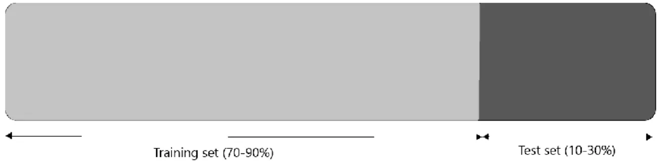
ML algorithms have successfully been implemented in a wide range of different applications such as: Speech recognition, fraud detection, games, medical diagnosis etc [13]. To be able to implement ML algorithms, relevant data sets must be collected [14]. ML algorithms are computational methods who performs accurate predictions or performance improvements based on experience [13]. The experience of an ML algorithm is gained from collected data sets, also called training sets. The data set should consist of different relevant features to the area investigated, the collected data is also known as a feature matrix. The ML algorithms can effectively learn from suitable features of the feature matrix, that is why the feature selection is an important step in ML. The collected data set is then divided into a training set and a test set. The sizes of these sets vary, but the training set is usually larger than the test set, seen in [Fig. 4]. Based on the training set the ML algorithm will learn which features that belong to which classes. The test set is used to determine the performance of an ML algorithms accuracy to predict the classification of features based on experienced from the training set.
In ML there are mainly two types of algorithms and their functionality varies [13]6. Supervised learning
is the most common ML technique and it consists of outcome variables that are predicted based on a given training set. The input values are then mapped into selected outputs (Labels or classes). Supervised ML is used for classification or regression. A few examples of supervised learning algorithms are: K-Nearest-Neighbour (KNN), Regression algorithms, Support Vector Machine (SVM) and Decision Tree. Unsupervised learning algorithms do not have any predicted outcome, it is used for clustering data into different groups. Apriori algorithm and K-means are two examples of unsupervised learning algorithms. The classification accuracy of the ML algorithms might depend on which kernel method the algorithm uses [22]. There are several different kernel methods that a ML algorithm could rely on in order to structure or separate the data better. However, in order to choose the most appropriate kernel and its setup depends on the data the ML algorithm is analyzing. The most common kernel methods are: Linear kernel, Polynomial Kernel, Gaussian Kernel. ML algorithms using different kernels with different tunings might increase or decrease the accuracy of the classification algorithm.
6 https://www.analyticsvidhya.com/blog/2017/09/common-machine-learning-algorithms/
The KNN algorithm classify in the feature space, the classification and regression are based on the closest training examples [23][24]. KNN is a lazy learning algorithm, this means that the KNN algorithm waits until the classification before doing its calculations and furthermore does its estimation’s locally. In order to use the KNN a training data set is needed, but during the training no learning is needed. Also, the algorithm has no need for an actual model during this phase. This means that the training data is needed for the testing phase and the data points do not have to be altered. When KNN tries to predict the unknown points, it votes by using the voting schema seen in [eq. 4]. Where (𝑥𝑛, 𝑦𝑛) represents pairs
of data n, 𝑥𝑛 is a feature vector and the 𝑦𝑛 is closest target class.
d(𝑥
𝑛, 𝑦
𝑛) = √(x
1− y
1)
2+ (x
2
− y
2)
2+ ⋯ + (x
𝑛− y
𝑛)
2(4)
When a point’s class is unknown the KNN algorithm calculates the closest neighbors based on the K value that is set [23][24]. If the K value is set to three, the three closest neighbors are included in the voting to classify the unknown data point, as shown in [Fig. 5]. To know which classified data points that are the closest can be done by assigning all data points a weight using a weight schema.Figure 5. The figure shows the KNN algorithm where the k value is set to three and the point with the question mark will be classified as blue even though the red point is closer. This is because the classification is done by a voting system and there are two blue point inside the closest circle which is determent by the k value.
SVM is a supervised learning technique, which tries to separate clusters of a data set by creating a boundary between them [25][26]. SVM does this by locating a decision function that can to separate the training data into different categories with equal distances between each other. If the decision function fails to find an appropriate distance between the clustered data, a softmargin is forced between the training data. After the training data has been separated the SVM selects where to draw the boundary in order to classify the clustered data. In linear SVM the boundary (hyperplane) can be drawn between the clustered data 𝑥⃗ as long as it satisfies the [eq. 5], where 𝑤⃗⃗⃗ is normalized vector to the hyperplane and b is a fixed offset from the origin to the vector 𝑤⃗⃗⃗.
𝑤
⃗⃗⃗∙ 𝑥⃗ − 𝑏 = 0
(5)According to Hussain et. al. [12] CL detection is a challenging task because of the factors that occur naturally in everyday life situations. There is also very inefficient for humans to manually review large data sets. This is where classification algorithms come into play, a classification model can be trained on data set constructed of psycho-physiological parameters (HRV, pupil dilation, EEG) where different levels of cognitive load should be obvious, such as: High, Medium and Low cognitive load.
Based on how well the trained model can predict data from a test set into the correct cognitive load level or class. The accuracy of the trained model is determined by how many misses and correct predictions the classifier chose from a test set. Studies has proven that the most common standard of measuring accuracy of binary classification of different cognitive states is the test accuracy [27]. There are many other metrics that are used in detection of cognitive states, such as the sensitivity and specificity measure F1-score that is the commonly used in medical field and is shown in [eq. 6]. Where recall is the number of of true positives divided by the number of condition positives, and precision is the number of true positives divided by the predicted positives. True positive is a correctly identified feature. However, there is no best accuracy metric in ML, all metrics have advantages and disadvantages in different situations.
𝐹
1= 2 ∙
𝑝𝑟𝑒𝑐𝑖𝑠𝑖𝑜𝑛 ∙𝑟𝑒𝑐𝑎𝑙𝑙𝑝𝑟𝑒𝑐𝑖𝑠𝑖𝑜𝑛+𝑟𝑒𝑐𝑎𝑙𝑙 (6)
Figure 6. The figure show how SVM creates a hyperplane is to classify clusters of trained data, as well as the parameters that are needed to calculate the hyperplane.
3. Related Work
3.1. State of the art CL domain
In a study performed by Nourbakhsh et.al. [28], they have analyzed different GSR features to detect four different levels of CL. During the data collection phase, the GSR device was connected to the index and middle finger on the left hand. The data was collected from two experiments. Two different ML algorithms were used to classify CL levels from the collected data, Naïve Bayes and SVM. The GSR features that were used was: peak number, peak amplitude, rise duration, peak area, accumulative and frequency power. The results showed that the features can be used to detect four levels of CL with high accuracy during affective changes. The two best GSR features in all situations were rise duration and accumulative. All the features had more than a 40% accuracy with at least one of the classification algorithms. The largest difference in accuracy for naïve Bayes and SVM was for accumulative GSR feature. The accuracies for the four different classes of CL was: rise duration (naïve Bayes: 57.9%, SVM: 55.3%), accumulative (naïve Bayes: 56.6%, SVM: 52.6%), peak number (naïve Bayes: 44%, SVM: 47%), peak amplitude (naïve Bayes: 47%, SVM: 44%) and frequency power (naïve Bayes: 39.5%, SVM: 34.2%). Which proved that naïve Bayes is better at classifying four different levels of CL. When conducting research on psycho-physiological parameters of test subjects in driving situations, they are commonly divided into field studies [29][30][31] and simulator studies [29][31]. There are adventages and disadvantages to both, but the advantage with simulator studies is that they are often feasible to convert into controlled experiments. Where the environment can be controlled at a higher rate then in a field study. However, the disadvantage is that the test subject doesn’t give simulation the same attention as if it was out in the filed. Solovey et. al. [29] continues by conducting filed studies while measuring psycho-physiological data (HR and skin conductance response) and the performence data in real-time without disturbing the driver. When combining the two different data types in the classification, they achieved a higher accuracy than when only using one type of data. In order to classify the data, five different ML algorithms were used, decision tree, logistic regression, multilayer perception, naïve Bayes, and KNN. Inorder to get reliable and robust data, 26 test subjects took part in the experiment and 13 of them gave both reliable HR and skin conductance response. From this they achieved up to 89 % accuracy using naïve bayes with 10 k-folds cross validations when classifying from both the psycho-physiological signals and the driving performance. The division av training and test data was 90/10%.
Because of safety and comfort concerns while monitoring CL in driving situations. Liu [32] have focused on the feasibility of using visual attention features to classify CL. The experiment was conducted by 37 test subjects in order to capture 3 different levels of CL, to capture this a faceLAB eye-tracker was used, also, EEG, ECG, GSR and respiration sensors (RESP sensor) were attached to the test subject. From the faceLab eye tracker where four Meta-features extraxted. Total number of gazes of center, count of gaze of center, total duration of eye elosure and count of blinking times. To collect the data, three different scenarios were used to simulate the driving senarios on thee 37 test subjects. The experiment was to drive around a course and for the secondary task was to count the number of times two identical letters appearing on the screen at the same time. Also, count the number of times two identical letters appeared with a letter in between the identical ones. The results were divided in to both binary and multi classification, for binary classification four metrics were taken note of: F2 score, accuracy, precision and recall was used to evaluate the different ML algorithms. Which were: KNN, logistic regression, SVM, adaptive boosting and random forest. Where KNN received the highest scores in the no grouping cross validation, 81 % accuracy was achieved and with an F2 score of 82%. A study on how connections between EEG-based CL and test subjects self-reported CL in a multimedia condition have been conducted by Chang et.al [33]. A controlled experiment involving two different educational tasks were used in order to collect data. In these two experimental phases the test subjects watched two different educational audio-based and video-based recordings. During the experimental phases an EEG helmet (NeuroSky) was used in order to measure the test subject’s theta/alpha ratio. 15
test subjects were involved in the data collection phase in the ages between 20-30. After the test subjects were done with the controlled experiment, they were given a CL questionnaire, where they filled in how they perceived the CL variation. The correlation between the self-reported CL and the measured CL with EEG was not similar. The amount of CL the test subjects thought they perceived could not be compared with the EEG’s detected cognitive load.
According to Kim et.al [1] the main cause of traffic accidents is cognitive load. They researched how brain activity is affected by CL during emergency situations while driving. EEG was used in order to detect how cognitive load affected the brain activity. Three test subjects were involved in a controlled experiment using a driving simulator. The controlled experiment was divided into two different phases. In the first phase the test subjects were instructed to follow a lead car, and then emergency break when the lead car slowed down. In the second phase they were instructed to do the same thing, although this time they had to listen to an audio book and count the number of words being said. EEG was measured during the controlled experiment through electrodes placed on the test subjects head. Time domain event related brain activity features were used in order to classify different levels of CL. The regularized linear discriminant analysis method was used as a classifier method. In order to classify the two different levels of CL was measured with a 5-fold cross-validation method was used. Area under the roc curve (AUC) scores were used in order to determine the classification accuracy. The AUC scores were not significant, in future works more features were to be included.
A study performed by Wang et. al. [34] has received a 97.2 % classification accuracy in detecting high cognitive load. The ML algorithms used were KNN, SVM, decision tree, random forest and XGBoost. Based on HRV and pressure relief valve (PRV) a feature fusion framework was used. In order to collect HRV and PRV data a controlled experiment was conducted where 160 test subjects were involved where each subject had to perform a 3-hour long mathematics test. Both ECG and photoplethysmogram (PPG) were recorded simultaneously in order to measure RR intervals and based on the RR intervals both the HRV and PRV was extracted. The PRV and HRV features extracted from the time domain were: Average of all RR intervals (AVNN), SDNN, RMSSD, PNN50, SDANN and the average of the RR interval standard deviations (SDNNIdx). The features from the frequency domain were: TotalPower, VLF, LF, HF and LF/HF ratio. In order to remove unnecessary features, the Fisher’s Linear Discriminant Analysis (LDA) was used. A pre-processing phase was introduced in order to filter the PPG and ECG signals while collecting data. The feature fusion tools used in this research were Procalcitonin (PCT), Sparse Kernel Reduced Rank Regression (SKRRR), Alternating Direction Method of Multipliers (ADMM), Linear Feature Dependency Modeling (LFDM). In order to classify different levels of high and low CL, Poincare plots were used. To determine the best combination of classifier algorithm and feature fusion tools with the collected data, specificity and sensitivity (F1 score) metrics were used. The classification accuracy using XGBoost classifier and the LFDM fusion tool was 97.2%, which outperformed every other classifier.
McDuff et. al [35] has built a remote person independent classifier in order to predict CL. The classification accuracy of their model was 85%. A contact-free camera-based system was used in order to measure HR, HRV and breathing rate (BR). The camera system could calculate these features by exploiting the capability of capturing the five-color band red, green blue, cyan and orange (RGBCO). In order to capture the source signals from the color band and to calculate the IBI, the independent component analysis (ICA) was used. Based on IBI, the HRV features could be calculated. Data was collected with the camera system in a controlled experiment divided into 2 phases. 10 test subjects were involved in the controlled experiments, each phase was recorded for 2 minutes. The first experimental phase was a normal sitting phase, and in the second phase the test subjects solved mathematical arithmetic. The features included in this research was mean HR, mean BR and LF, HF and LF/HF ratio. Two ML algorithms were used in order to classify the two different levels of CL. Naïve Bayes achieved an 80% classification accuracy and SVM achieved 85% classification accuracy.
3.1.1. How controlled experiments involving video games are conducted
To assess the worth of CL, as much information as possible needs to be known
[36]. Therefore, every possible detail needs to be accounted for before doing experiments in CL domain, if the information is not needed after the experiment is done, it can be discarded. But if something key is missing from the experiment the whole experiment could be meaningless. To get the useful information out of an experiment, it is vital to write down and describe everything to the utmost. When Xiao et. al. [17] did their experiment, they designed their experiment to answer the hypothesis. The hypothesis was trimmed down into bullet points and could be answered with a yes or no but could also be more elaborately answered. After this the test subjects information were stated: gender, age, place of work, background with similarity to the task at hand, right- or left-handed, their health, medication, history of psychological-, neurological-, cardiovascular-diseases. The course of action and settings for the game were detailed as well. Xiao et. al. [17] specified the conditions that the test subject was in when taking the test: what they were sitting in, room temperature and noise level in the room. After the experiment was done the test subjects had to answers a questionnaire about the effort, they felt that they put into the completion of the tasks they did in the experiment. The experiment consisted of four different stages, rest, first-, second- and third wave of the game. The test subjects where monitored with an PPG sensor located on the left index finger. In order to capture what the test subject saw at any given moment, the screen where also filmed. This was done to analyze if anything triggered more CL and to compare a certain moment in the test with the test data.
3.2. The camera system
Non-contact health monitor systems have been incessantly growing in the research community [9]. One of the systems that have been explored is the camera that was a pioneer for non-contact free based system. The camera system Rahman et. al. [9] have developed works both in real time and in offline, where the system uses color schemas such as RGB and Lab. Using this system, the HRV can then be calculated which can be used for detecting fatal diseases, but also to estimate stress level and CL. The HRV is calculated by extracting the RGB color form the variation in the facial skin of the test subject. The recorded data from the camera gives an average value of the colors of the Lab space, these are extracted with a sampling frequency of 12 Hz for every frame. However, the HR and IBI where recorded with a sampling frequency of 4 Hz directly. When calculating the HRV, Rahman et. al. [9] used a remote Matlab script that both took the raw data and saved the calculated data in a MySQL database server. The desired region of interest (ROI) is a zoomed in region from just above the mouth to the heir line in the vertical direction and in the horizontal direction the region goes from eye to eye [9]. The full ROI is 80 percent of height and 60 percent of width of the face. For the face detection they used Viola and Jones algorithms for the ROI, and they used it for every frame in that region. The Lab color space that the RGB values was converted into from the ROI, are L (represents the lightness), a and b (represents color-opponent dimensions, that are based in non-linearly compressed coordinates). Rahman et. al. [9] discards the signal L to account for the environmental illumination, this because the a and b signal can filter the ambient illumination. Based on this the signal is filtered using a band pass of 40 – 120 Hz and is also normalized. To extract the HR and IBI and obtain the average value of them, three different algorithms was used PCA (Principal Component Analysis), FFT (Fast Fourier Transform) and ICA (Independent Component Analysis). Also, for calculating the HRV both time domain and frequency domain was used.
3.3. Analysis and Comparison
To summarize the main points in the state-of-the-art research from the CL domain section 3.1 and 3.2 • There are contact-free measures that can extract HR and IBI based on GSR and eye-tracking. • ECG, GSR and PPG are common contact-based measures to detect CL. However, the most
common measure of CL is EEG.
• The psycho-physiological parameters extracted through the above stated measures are: PRV, HR, BR, IBI, skin conductance and pupil dilation. Where HRV and brain activity is the most common.
• The most common HRV features are: LF, HF, SDNN, RMSSD, etc.
• Simulator studies (Controlled experiments) is the most used for data collection, but CL has also been measured in field studies.
• In order to detect different levels of CL the experiment is divided into atleast 2 different phases, with varying levels of cognitive distractions.
• It is important to account for more then needed test subjects when conducting experiments, because some of the data can be unusable.
• It is important to gather as much information as possible, methods used for this are: background questionnaire, what happens around the test subject, take note of what the test subject experienced, etc.
• The most common secondary task while already performing a main task is to either count or completing math questions.
• In order to have have a realiable accuracy, atleast two ML algorithms need to be used in a classification of CL.
• The most common ML algorithms in the CL domain are: SVM, naïve Bayes, KNN, random forest, decision tree, logistic regression.
• When comparing ML algorithms, mean accuracy is the most common unit, but F1 score are also used for binary classification as well as AUC.
• Division of training and test data are usually: 80/20%-90/10%
In this thesis the state-of-the-art process will be followed, it will start with a data collection phase, where HRV features using a contact-free system developed by Rahman et.al [9] stated in chapter 3.2 using GSR will be extracted. Where the ROI is important to not overlook when conducting the experiments. To have something to compare the contact-free system with a contact-based system will also used to measure GSR in order to determine which one that can extract CL better from test subjects. As the stat-of-the-art mentions its important to have different phases in the controlled experiment, also to take note of every detail. If there is a desired amount of test subjects that are needed when conducting the controlled experiment, it is important to have a few more than needed. This is because of the fact that some of the test subjects might not give readable data for the ML algorithms to classify. When classfying the collected data it is also important to use more than one ML algorithm. To compare the ML algorithms there are two more common ways of comparison, which is the mean accuracy and the F1 score. A divided training set and test set in the span of 80/20% or 90/10%.
What will be excluded from this thesis:
• Meta-features and non-linear HRV features and feature fusion tools feature. • Eye-tracking, ECG, EEG and PPG.
• Audio-based and video-based recordings in the controlled experiment. • Field studies
4. Problem Formulation and Research Questions
Scientists argue that the best approach in detecting CL is EEG, since it can detect the amount of mental workload that is spent on certain tasks by measuring electrical activity in the brain [5]. However, EEG: s drawback is that it is too cumbersome in certain situations (such as driving) since it needs to attach wired electrodes to the head of the test subject [8]. This is a problem that might affect the results, where the experiment already might have emotional and environmental variables that can affect the result [12]. However, there are other less cumbersome contact-based approaches that can be used to detect CL, that are based on other psycho-physiological parameters, such as ECG and GSR. However, the problem remains, they are contact-based and emotional as well as environmental variables might still affect the results [12] [8]. That is why a contact-free system using a regular camera to extract HR and IBI recently was developed. This contact-free approach should be possible to use to detect CL based on HRV features, which could be very beneficial in CL detection. However, when identification of CL is done by humans it is not efficient [12], this is where ML algorithms could play a vital role. ML algorithms makes it possible to classify different levels of CL based on large datasets with HRV features. To determine the performance of the contact-free system in detecting CL, a contact-based approach using shimmer Sense that extracts HR and IBI will be used to compare it with. Based on different HRV features, 2 different ML algorithms are going to be implemented in order to see which one is better at classifying three levels of CL.
The challenges that will be faced in this thesis are:
• Synchronizing the two different approaches while collecting data
• Perform a large datacollection with both approaches in a controlled experiment as well as implementing and analyzing the results in a small timespan
• Select optimal HRV features for the collected data
• Extract features from the collected data both in the time-domain and the frequency-domain • Implement ML algorithms and optimize them for the collected data
This leads to the core research questions of this study:
• How accurate can CL be identified based on extracted HRV features using a contact-free system (the camera system)?
• Does the contact-free system (the camera system) identify human CL better or worse than a traditional contact-based sensor system (shimmer sense GSR+)?
• Which of the classification algorithms KNN and SVM, is the most accurate in detecting CL in this situation?
Goals:
• Measure IBI properly with both the contact-free and the contact-based systems. • Collect sufficient robust data (IBI and HRV, timestamps) using both systems. • Investigate how to perform experiments ethically correct.
• Implement at least two different ML algorithms to see which ones are better at classifying CL in this particular situation.
• Find the two best ML algorithms for the collected data
• Extract HRV features using the frequency domain methods as well as the time domain methods. • Prove if it is possible to get robust CL data by using a fast-paced game in the experiment. • Manage collected data from the controlled experiment and convert it into a feature matrix that
5. Materials and Method
In this thesis the free system developed by Rahman et. al. [9] will be compared with a contact-based shimmer sense GSR+ measuring system to see if the camera-contact-based approach is as good or better than a contact-based approach. Also, investigate how accurately the KNN and SVM algorithms can classify different levels of CL based on data gathered by the two approaches from the controlled experiment. This will reveal which of the classification algorithms that is the most suited for the collected data from the controlled experiment. In order to preforme this thesis, two scientific methodology where chosen, controlled experiments and state-of-the-art research. The controlled experemnts where used to collet robust and reliable data. The state-of-the-art research was preformed to give the thises a thorough foundation in which the theis is built upon.
Shown in [Fig. 7] is a block diagram that describes the different processes in this thesis, they are performed in order to answer the research questions stated in the problem formulation. The first phase is the data collection, which was conducted by recording the test subjects in the controlled experiment. The data collection flow will be explaned in this chapter 5, also go into detail about the setups of the equipment. The remaning blocks (Data Processing, Data Set Preparation, Classification Learner, ML Algorithms, Model Classifier and Classification Results) of the diagram shown in [Fig. 7] will be explained in chapter 7 (Implementation) and 8 (Results).
5.1. Controlled experiment setups
When setting up the controlled experiment the positions of where everything related in the room was located was measured to get the experiment as similar as possible for everyone. The chair that the test subjects were stationed in during the experiment was positioned centered in front of the television (tv) and the table was in front of the chair. The backrest on the chair was positioned 225 centimeters (cm) from the tv screen and the seat of the chair is 46 cm off the ground. The chair is cushioned both in the seat and the backrest with no armrest. The table that was used in the experiment was not the table that was bought with the chairs, but it had the same height as that table. It was a stable table but when the test subjects leaned heavy enough on the table, it shook, but not enough to interfere in the experiment. The table has a height of 72 cm and the camera was adjusted to stand 34 cm above the table to get a better angle of the face (if it was a shorter test subject, the camera was adjusted, about 10-15 cm lower). The length from the backrest to the camera was 90 cm. When the test subjects were taking the experiment, they moved back and forward with the head but when they sat with the back to the backrest their face was about 70 cm away from the camera. The working area on the table was 51 cm in depth and 120 cm in width. The test subjects had different heights, but their eyes were located 50 cm -+10 cm above the table. The controlled experiment environment and all the setups can be seen in [Fig. 8]
5.1.1. Shimmer Sense
The shimmer sense system, that was used during the controlled experiment was a Shimmer3 GSR+ seen in [Fig. 9]. It was connected to the body through a clamp to the earlobe. Based on GSR, the shimmer device could measure the IBI and HR etc. in real time. Shimmer3 uses a software called Consensus to monitor and manage the data gathered by the shimmer sense. The data recorded by the shimmer sense can be extracted to the PC in two different ways, either through Bluetooth or USB. The shimmer sense records information which can be stored in an Excel file. The standard settings of Consensus were recorded in: Unix_Timestamps, GSR_Range, GSR_Skin_Conductance, PPG_A13 and PPGtoHR. However, in Consensus it was possible to change setting in order to record IBI’s. The standard recording settings for the shimmer sense besides adding the IBI’s. The shimmer had a sampling rate of roughly 40 000 rows in an Excel sheet from a 5-minute test run.
5.1.2. Camera
The camera that was used to record videos of the test subjects during
each phase of the controlled experiment was a Logitech HD Webcam C615. The camera records with a resolution of 1920x1080, and a frame rate of 30fps equipped with auto focus. The software used to manage the data recorded with the camera was Bandicam. The recordings from the webcam was stored as MP4. The test subjects of the controlled experiment sat roughly 70cm in front of the camera during the different phases of the controlled experiment. The camera was adjusted according to the height difference between the head of the test subject and the camera was about 20cm. This was to get the desired ROI of the test subjects facial features [9]. Before the controlled experiment began, the test subjects were told to don’t move their heads too much while they were recorded. This was especially important while the test subjects solved the metal puzzles. The reason for this was that the camera system needs a straight angle of the face in order to calculate the IBI. The process of how the camera system extracts IBI from a video recording can be seen in [Fig. 10]
Figure 9. The Shimmer3 GSR+ device
Figure 10. Diagram describing the different processes of how the camera system extracts IBI from a video recording.
5.2. Data collection (controlled experiments)
To collect data that could be used to create feature matrixes to feed the ML algorithms, controlled experiments was chosen to answer the core questions stated in the problem formulation. Controlled experiment was chosen because of the importance to control the environment the experiment is taking place in to minimize affective variables [17]. To ensure that both approaches could measure the IBI properly, test runs were conducted on different phases of the experiment. In order to test the robustness of the data collected with both systems, three different phases from the controlled experiment was chosen. Since the camera-system can be used in offline and the camera system was not available at the time of when the test runs were conducted, the videos were recorded locally. The testing revealed that the shimmer sense didn’t record any IBI. Which resulted in some changes in the shimmer sense software, to record both IBI and HR. During the controlled experiment the test subjects was recorded via a webcam, and they were wired up with the shimmer sense. The controlled experiment consists of seven phases, in-between each phase there will be a minor pause to set the next phase up and in the fifth phase there will be a 15-minute break, see [Fig. 11].
The first phase of the experiment is going to be a five-minute rest while sitting normal watching tv noiselessly. Then, in phase two the test subject is going to complete two different easy metal puzzles while sitting normal. In the second phase the test subject will start with the first easy puzzle, and when they have dissembled the first one, they started on the next one. When both puzzles are dissembled the test subject would start to reassemble both puzzles in the same order. This process was repeated for five minutes. Phase three is the same as phase two but both metal puzzles were at a higher difficulty. In phase four the test subject rested for 15 minutes and were offered coffee and snacks. During the fourth phase was the only time the test subjects were allowed to remove the measuring systems. After the 15-minute break the test subjects were wired up again, and the fifth phase was started. In the fifth phase the test subjects were going sit normal watching noiseless tv just like in phase one, for five minutes. In phase 6 the test subjects were going to play Mario Kart Double Dash on the 150cc course BOWER´S CASTLE competing against seven bots. The time of this phase varied depending on how well the test subjects performed, the mean time was about 3:45 minutes. In phase seven the test subjects were going to play Mario Kart Double Dash 150cc once again, but on RAINBOW ROAD, which is the final and the hardest course of the game. Once again competing against seven bots but this time the test subjects had to answer math questions while driving. The math questions had to be answered before the next question was asked, the questions were asked every 30 seconds with five questions in total.
During the different phases of the controlled experiment, notes of everything that happened was written down, even trivial information. This was done to be able to backtrack if something might have affected the recorded data. For instance, if the test subject became tired or needed to go to the bathroom which could affect the HR [12]. However, before the test subjects were involved in the controlled experiment, they had to sign a contract and fill out a background questionnaire. The contract stated that their involvement could be withdrawn at any given moment, if they so choose and that their personal data won’t be shared [36]. The test subjects that agreed to show their face in this thesis were informed that their results will be presented in a fashion where they will be anonymous. Both the background questionnaire and the contract can be seen in Contract and Background Questionnaire in the Appendix A and B.
11 test subjects performed in the controlled experiment, atleast ten people was desired, one extra test subject was added in case any recordings were corrupted and had to be discarded. This resulted in 12 recordings per test subject, six for each approach. The shimmer sense stored data in Excel sheets, and the videos from the camera was stored in MP4. The data collected during the controlled experiment was only stored locally to protect the involved test subject’s integrity to the utmost. The test subjects that took part in the experiments were in the ages from 21 to 33 years old, 9 of them were men and two of them were women. The average age of men was 26 and for women 27. The level of education was divided into two groups where 6 people had a higher education than gymnasium, but all 11 test subjects had a gymnasium degree. Of the total 11 people, the four people that had the lowest education in math had read up to B (in old system)/2c (new system). The three people with the highest math education had read to or over math D (old system)/3c (new system) and added to this a few college math courses. The mean value of how good they see themselves in mental arithmetic were 5,9 in a scale to 10. The mean value of time spent playing digital games per week was 13 hours, but the time differed a lot between the test subjects. The one with the highest hours per week had 40 hours, and the lowest had one hour. 2 of the 11 only played on mobile, and the rest played on console/computer. All the test subjects had tried a Mario Kart game in their life but 9 out of 11 had tried Mario Kart Double Dash. The mean value of how good they saw themselves on a scale to 10 was 3,9 in Mario Kart Double Dash. All test subjects were unfamiliar with the metal puzzles, they answered that on a scale to 10 the mean value was two. It was 4 of the 11 test subjects that had never seen a metal puzzle before. All the test subjects answered that they were healthy when partaking in the experiment and had no history of psychological, neurological or cardiovascular diseases. One test subject answered that he/she could get migraine, and another wrote that he/she had gotten a concussion one year before. 5 of the 11 test subjects said that they consumed alcohol in the past two days. Because of the high answered rate of this question it was investigated, and the the five test subjects were questioned in more detail when they consumed the alcohol. All of them answered that they consumed the alcohol the second day prior. This high answered rate was because the controlled experiment was conducted mostly on the Easter weekend.
The mathematical questions were in three sets, one test subject only answered one of them. It was random which set the test subject got, the questions can be seen in [Fig. 12].