Microstructure and deformation behaviour of ductile iron under tensile loading

(1)

LICENTIATE THESIS

Microstructure and deformation

behaviour of ductile iron under tensile

loading

Keivan Amiri Kasvayee

SCHOOL OF ENGINEERING, JÖNKÖPING UNIVERSITY Jönköping, Sweden 2015

Department ofMaterials and Manufacturing

(2)

Microstructure and deformation behaviour of ductile iron under

tensile loading

Keivan Amiri Kasvayee

Department of Materials and Manufacturing School of Engineering, Jönköping University SE-551 11 Jönköping, Sweden

Research Series from the School of Engineering, Jönköping University Department of Materials and Manufacturing

Dissertation Series No. 9, 2015 ISBN 978-91-87289-10-1 Published and Distributed by

School of Engineering, Jönköping University Department of Materials and Manufacturing SE-551 11 Jönköping, Sweden

Printed in Sweden by Ineko AB

(3)

ABSTRACT

The current thesis focuses on the deformation behaviour and strain distribution in the microstructure of ductile iron during tensile loading. Utilizing Digital Image Correlation (DIC) and in-situ tensile test under optical microscope, a method was developed to measure high resolution strain in microstructural constitutes. In this method, a pit etching procedure was applied to generate a random speckle pattern for DIC measurement. The method was validated by benchmarking the measured properties with the material’s standard properties.

Using DIC, strain maps in the microstructure of the ductile iron were measured, which showed a high level of heterogeneity even during elastic deformation. The early micro-cracks were initiated around graphite particles, where the highest amount of local strain was detected. Local strain at the onset of the micro-cracks were measured. It was observed that the micro-cracks were initiated above a threshold strain level, but with a large variation in the overall strain. A continuum Finite Element (FE) model containing a physical length scale was developed to predict strain on the microstructure of ductile iron. The materials parameters for this model were calculated by optimization, utilizing Ramberg-Osgood equation. For benchmarking, the predicted strain maps were compared to the strain maps measured by DIC, both qualitatively and quantitatively. The DIC and simulation strain maps conformed to a large extent resulting in the validation of the model in micro-scale level.

Furthermore, the results obtained from the in-situ tensile test were compared to a FE-model which compromised cohesive elements to enable cracking. The stress-strain curve prediction of the FE-simulation showed a good agreement with the stress-strain curve that was measured from the experiment. The cohesive model was able to accurately capture the main trends of microscale deformation such as localized elastic and plastic deformation and micro-crack initiation and propagation.

Keywords: Ductile iron, digital image correlation (DIC), in-situ tensile test, pit etching, Micro-scale deformation, micro-crack, finite elements analysis (FEA), cohesive elements

(4)

(5)

ACKNOWLEDGEMENTS

I would like to express my sincere appreciation to all the people who have helped me along the way of my PhD studies:

My supervisors, Professor Anders E.W. Jarfors, Dr. Ehsan Ghassemali and Assistant Professor Lennart Elmquist for providing support, guidance, insightful discussions and valuable education.

Associate professor Kent Salomonsson, for his invaluable work in performing simulations, and patiently teaching.

The technicians, Toni Bogdanoff, Lars Johansson and Esbjörn Ollas for helping me with the experimental work.

The Knowledge Foundation for financial support under the CompCAST project (20100280). The industrial partner SKF Mekan AB and their helpful personnel especially Björn Israelsson for providing the project with the cast material.

All my friends and colleagues at the Jönköping University for creating such a pleasant work environment.

My beloved family, especially my parents, and good friends for their support, motivation, comfort and for providing me with joy and happiness in my life.

(6)

(7)

SUPPLEMENTS

The following supplements constitute the basis of this thesis.

Supplement I K.A. Kasvayee, L. Elmquist, A.E.W. Jarfors, E. Ghassemali.

Development of a pattern making method for strain measurement on microstructural level in ferritic cast iron. PFAM XXIII. India, 2014.

K.A. Kasvayee was the main author. L. Elmquist, A.E.W. Jarfors and E. Ghassemali contributed with advice regarding the work.

Supplement II K.A. Kasvayee, E. Ghassemali, A.E. Jarfors. Micro‐Crack initiation

in high‐silicon cast iron during tension loading, TMS2015 Supplemental Proceedings 947-953.

K.A. Kasvayee was the main author. E. Ghassemali and A.E.W. Jarfors contributed with advice regarding the work.

Supplement III K.A. Kasvayee, K. Salomonsson, E. Ghassemali, A.E. Jarfors.

Microstructural strain distribution in ductile iron; comparison between finite element simulation and digital image correlation measurements. Submitted to the journal of Materials Science and Engineering: A.

K.A. Kasvayee was the main author. K. Salomonsson performed the optimization and FE-Simulation. E. Ghassemali and A.E.W. Jarfors contributed with advice regarding the work.

Supplement IV K.A. Kasvayee, E. Ghassemali, K. Salomonsson, A.E. Jarfors.

Microstructural strain localisation and crack evolution in ductile iron. JTH research report ISSN 1404-0018, Jönköping University. K.A. Kasvayee was the main author. K. Salomonsson performed the FE-Simulation. E. Ghassemali and A.E.W. Jarfors contributed with advice regarding the work.

(8)

(9)

INTRODUCTION

CHAPTER INTRODUCTION

This chapter describes the background for the current work by focusing on fundamental, microstructure, crack evolution, deformation properties and simulation of ductile iron.

1.1 DUCTILE IRON

1.1.1 Background

Ductile iron is a group of ferrous materials among the cast iron family containing nodular shape graphite particles, which is also known under the names of nodular iron or spheroidal graphite (S.G.) iron [1]. This material has been developed and used since 1949, when H. Morrogh at the British Cast Iron Association for the first time reported how to change the lamellar graphite of grey cast iron into spherical shape [2].

Ductile iron has some superior properties such as high strength, good castability, good machinability, high toughness and low cost. It obtains its good properties by means of its specific chemical composition, matrix and nodular graphite. Depending on the matrix microstructure, ductility and tensile strength of ductile iron can raise up to 18% and 850 MPa, respectively [3]. These good properties have made ductile iron a strong candidate for a vast range of applications such as constructive and automobile industries.

Ductile iron is a ternary Fe-C-Si alloy with a typical C and Si content of 3.5-3.9% and 1.8-2.8%, respectively. During the solidification, the carbon in excess of its solubility in solid iron forms graphite. Nodular graphite can be produced by small addition of magnesium or rare earth elements to the cast iron during melt treatment. The big advantage of nodular graphite is its round edges (despite the sharp edges of lamellar graphite) that not only reduces the risk of crack initiation, but also acts as a crack arrester and increases crack propagation resistance; thus, promotes higher toughness, fatigue resistance and impact resistance [3, 4].

The amount of nodular graphite depends on carbon equivalent (Ceq) and cooling rate during

the solidification. Carbon equivalent is an empirical value, which converts the amount of alloying elements to an equivalent percentage of carbon [5]. Carbon equivalent mostly depends on the C, Si and P contents and can be calculated from Eq. (1) [6].

Ceq = C% + 1/3 (Si% + P%) (1)

1.1.2 Microstructure

The final microstructure of ductile iron highly depends on solidification conditions, chemical composition and casting method [7, 8]. Figure 1 shows a typical micrograph of ductile iron, which contains graphite in black circles, ferrite phase in white and pearlite structure as grey [9].

(12)

The black graphite nodules covered with white ferrite phase in ductile iron matrix is called “bull’s eyes” [4]. Depending on the chemical composition, ductile iron can be classified as eutectic (Ceq= 4.33), hypoeutectic (Ceq < 4.33) or hypereutectic (Ceq > 4.33) [7].

Figure 1. Typical microstructure of ductile cast iron, containing nodular graphite embedded in ferritic and pearlitic matrix [9].

The properties of ductile iron highly depends on the type of matrix phase, alloying elements and amount and shape of the graphite. Increasing the amount of ferrite in the matrix leads to higher ductility but lower strength. In contrast, higher pearlite content causes more strength and lower ductility [8, 10]. In order to minimize the amount of pearlite in ductile iron, pearlite promoting elements (e.g. Cu, Mn, Sn, Cr) should be minimized and ferrite promoting elements (e.g. Si) should be increased [11, 12].

General shape of the graphite particles (nodularity), the number of nodules per unit area (nodule count) and the overall graphite volume can affect the mechanical properties [13, 14]. In general, higher nodularity results in higher ductility and strength [10]. The amount and type of alloying elements can affect the mechanical properties by changing the matrix phase, nodularity and nodules counts. In addition, alloying elements can change the properties e.g. by solid solution hardening, changing the interlamerllar space of pearlite and stabilizing austenite at low temperatures [4].

1.1.3 Solidification

The iron-carbon phase diagram is presented in Figure 2 to illustrate the solidification process of ductile iron under equilibrium condition [5]. The eutectoid reaction is defined as a single-parent phase decomposing into two different phases through a diffusional mechanism. Eutectic is a reaction where a liquid phase transforms into a mixture of two solid phases. The iron-carbon system has a eutectic at composition of 4.3 wt%C at 1130˚C, which liquid iron directly transforms to austenite and cementite. The eutectic mixture of austenite and cementite is called Ledeburite [15].

(13)

Figure 2. Iron-Carbon equivalent phase diagram [5].

During solidification, assuming equilibrium cooling state for a hypereutectic ductile iron melt, the first solid to crystalize from the liquid is graphite phase. Graphite prefers to nucleate in low energy interface of inclusions or inoculants (e.g. MgS, CaS and MgO·SiO2). By decreasing

temperature down to the eutectic line, graphite particles gradually grow by depleting carbon from the melt area [5, 16].

During eutectic solidification, austenite nucleates in carbon depleted zones around graphite nodules and grows until fully austenitic matrix is achieved. After the eutectic transformation, more temperature reduction causes an increase in the graphite volume since the carbon solubility in austenite decreases from 2% at eutectic to 0.8% at eutectoid temperature and consequently the carbon atoms diffuse toward the preexisting graphite nodules [5, 16]. By passing the eutectoid temperature, more carbon diffuses to the graphite nodules because of transformation of austenite to ferrite which is accompanied by carbon solubility reduction to 0.02% (Maximum carbon solubility in ferrite). Ferrite prefers to nucleate at austenite-graphite interface where diffusion of carbon into graphite has made a carbon-depleted zone. Further growth of ferrite happens by diffusion of carbon atoms through the growing ferrite from austenite into graphite. Therefore, the resulting equilibrium microstructure will be ferritic matrix with graphite [5, 17].

The equilibrium microstructure can be achieved only when carbon has sufficient time and driving force for diffusing into the graphite. At higher cooling rates the carbon atoms do not have enough time to diffuse during eutectoid reaction. Thus, cementite nucleates at ferrite-austenite interface because of the higher carbon content of ferrite-austenite and initiate the formation of the pearlite. Pearlite grows much faster than ferrite due to much shorter distance between constitutes, ferrite and cementite. In other words, beyond a certain undercooling cementite growth prevails the graphite growth and mostly pearlite forms during eutectoid phase transformation [5, 17].

(14)

1.1.4 High silicon ductile iron

High silicon ductile iron is a type of ductile iron with silicon content around 4% . Silicon has a strong ferrite establishment attitude with a solid solution effect that increases the hardness, ultimate tensile strength and yield strength of ferrite and consequently improves the mechanical properties of alloyed ductile iron. Si has been considered as a graphitizer alloying element in ductile iron. It also increases the nodule count and as a consequent reduces the carbon diffusion path during the eutectoid transformation so that the amount of ferrite increases in matrix [5, 18]. In contrast to the most alloying elements, Si segregates into the solid phase during solidification (Negative segregation) [4].

Compared to the other grades of ductile iron, high silicon ductile iron has several advantages such as excellent machinability, higher hardness uniformity, higher corrosion resistance, higher tensile and yield strength. Although these properties make this material an appealing substitute for ordinary ductile iron in industrial applications, its poor ductility, low impact energy and brittleness have limited its applications [18, 19].

1.2 DEFORMATION BEHAVIOUR OF DUCTILE IRON

1.2.1 Microstructural deformation

Although the overall macroscopic deformation response of ductile iron has been regarded as homogenous, deformation in microstructure is fully heterogeneous [20, 21]. In-situ tensile tests [22-24] and its combination with DIC has been used to measure and characterize deformation and failure in microstructures. At micro-scale level, a strong strain partitioning and localization occurs in the constituent phases and between graphite particles [20, 25, 26]. This was attributed to the local variation in the microstructural features such as matrix (ferrite or pearlite) and graphite (shape and size) [27]. Such heterogeneity results in strain localization, leading to a scatter in the resistance of the phases against the micro-crack initiation and propagation. Ferrite is a high-ductility low-yield material and pearlite is a high-strength, low-ductility material. Therefore, higher localised deformations accumulate in ferrite phase compared to pearlite, since graphite nodules are typically embedded in the soft ferrite phase and act as local stress raisers. The lowest localised deformation occurs in pearlite areas since pearlite structure is the strongest constitute of the microstructure [28].

1.2.2 Crack initiation and propagation

The common knowledge on how cracks initiate and propagate in ductile iron can be characterized as follow: (i) development of the cracks inside graphite, (ii) decohesion between matrix and graphite at low stress and plastic strain, (iii) plastic deformation in matrix around graphite nodules which creates voids that grow by plastic flow, (iv) initiation and propagation of micro-cracks in the deformed matrix between graphite nodules, (v) linkage of graphite nodules via micro-cracks connections and hence formation of larger micro-cracks, (vi) further linkage of large micro-cracks and formation of macrocracks [29-31].

The graphite particles act as a nonmetalic secondary phase in iron matrix of ductile iron. As a fully elastic material, graphite does not deform plastically during the deformation of ductile iron. Accordingly, three types of internal cracking were observed for graphite particles during deformation: (i) decohesion of graphite from the metal matrix, especially from ferrite, (ii) a radial and transversal crack initiation and propagation at core zone of graphite nodules (mostly occurs in nodules with lower roundness), (iii) crack nucleation and growth between the graphite nodule core and the graphite outer shell [24, 32].

In the vicinity of graphite and matrix interface, the difference between elastic and plastic properties of the two phases can raise the mechanical stress and eventually cause interfacial

(15)

crack initiation [29]. The irregular surface and sharp corners of graphite can promote crack initiation [33]. Stokes et al. [34], considered the graphite/matrix decohesion as the critical micromechanism for initiation and growth of micro-cracks. This decohesion were mostly reported when a perfect round nodule was surrounded by ferrite phase [24, 35]. Nevertheless, there has been reports [20, 36], considering graphite nodules as rigid spheres that act like voids, which grow with strain and their coalescence results in large equiaxed dimples.

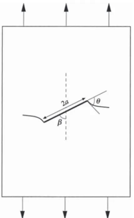
Considering crack propagation in the matrix of materials with a pre-existing imperfection, the crack which was nucleated at the imperfection can enter matrix and reorient to propagate on the plane with the highest normal stress, see Figure 3 [37]. Similarly in ductile iron, fracture can occur in graphite particles, which acts as crack nuclei for ductile or brittle crack propagation in the matrix [37]. The micro-cracks that have been initiated at the matrix/graphite interface propagate in the matrix. Micro-cracks link together and propagate in the paths between nearby graphite nodules [24].

Figure 3. Nucleation of crack in a pre-existing imperfection and crack propagation in matrix material. Crack reorient at matrix/imperfection boundary to propagate in plane with maximum normal stress

[37].

1.2.3 Fracture Surface

According to the fractographic observations in ferritic/pearlitic ductile iron [20, 38, 39], the fracture surface consists of three main features: First, equiaxed dimples surrounding each graphite nodule in ferrite phase. Each nodule acts as a void that subsequently grows with strain in a direction parallel to the applied tensile loading. Second, voids that are about one order of magnitude smaller than the primary dimples. These secondary voids were typically observed at the boundaries of the larger dimples and were found where the primary voids met or linked up. Third, typical cleavage facets of ferrous alloys, mainly in pearlitic area.

(16)

1.3 DIGITAL IMAGE CORRELATION

1.3.1 Background

DIC was first developed by a group of researchers at the University of South Carolina in the 1980s [40, 41]. Digital image correlation (DIC) is an optical-numerical measurement technique for determining complex displacement and strain fields on the materials surface under any kind of loading [42]. The distinct advantage of DIC compared to the conventional extensometers is the full-field strain measurement that can provide quantitative strain values across a broad range of length scales [42].

DIC correlates the grey values of a reference undeformed image with a deformed image to determine displacement and strain of the deformed image. The measurement can be done by comparing image series that are captured over a defined timescale, which can be from microseconds to years. Moreover, it is possible to measure displacements in different scale levels depending on the image scale. For example, microscope images can be used for measuring micro/nano scale displacements [43].

DIC can be categorized as two dimensional (2D) or three dimensional (3D). The 2D is generally capable of determining displacements in the image plane only, whilst the 3D variant enables the measuring of the all three (spatial) components of the displacement vector by adding an extra camera to the measurement setup [44].

1.3.1 Speckle pattern

The specimen surface must have a random speckle pattern that can deform with the surface as carrier of deformation information. Laser speckle patterns [45, 46] and artificial white-light speckle patterns (the random grey intensity pattern of the object surface) commonly have been used as speckle patterns [47]. The white-light speckle pattern can be obtained by the natural pattern of the specimen [28, 48] or black/white spray paint [26].

In micro-scale level, small size speckles are required. In this case, speckle pattern generation methods have been mainly based on photolithography [49], chemical vapour thin film patterning [49], laser patterning [50] micro/nano particles [51-53], fine paint [25, 53], etching and using natural microstructural pattern [48, 54].

Speckles size play a critical role to ensure a suitable balance between measurement accuracy (bias error) and precision (standard deviation error) [55]. A practical limit in size of the speckles is that the image’s speckles should be sampled at least by a 3 3 pixels array. If the speckle sizes become smaller than this limit, the camera sensors cannot properly sample the speckles’ light signals for image production, and eventually the correlation results will severely suffer from aliasing and low contrast bias errors [42, 56].

1.3.2 Subset and spatial resolution

In subset-based DIC programs, correlation occurs by considering a pixel and its neighbourhood, specified as subset in undeformed image (indicated in red square in Figure 4) and matching the same subset in the deformed image [57, 58]. Subsets have square shapes with side length of (2N+1) pixels, where N is a natural number. Subset size determines the minimum displacement area which can be resolved. Subset size must be large enough to contain unique and identifiable features. Too small subset will result in high uncertainty in correlation results whereas too large subsets will smooth out details in large heterogonous deformations and significantly degrade accuracy of the results [59, 60]. Lower limit of subset size is governed by granularity of the speckle pattern. The upper limit of subset size can be defined depending on the desired spatial resolution [59, 61].

(17)

Figure 4. Schematic illustration of a subset deformation in reference and deformed images [62]. A subset has been shown as a red square. The centre point P(x0,y0) can be considered to move with a displacement vector to P’(x’0,y’0) by transition. The Q(x0,y0) has been deformed to Q’(x’0,y’0).

Spatial resolution is defined as the smallest distance between two independent measurement points. Displacement spatial resolution is the subset size, since it defines the distance between two independent data points in correlation. The strain spatial resolution (SRS) is limited by the subset size used for correlation matching and by the measurement grid of strain concentration, which can be calculated from the Eq. (2). Step size (ST) is the distance between two adjacent displacement data points, which determines the data density of a displacement field. The strain window is the number of displacement data points that are involved for strain calculation. Strain window (SW) size in pixel dimension, denoted as virtual strain gage (VSG), can be measured from Eq. (3), which represents the smoothing area for strain measurements [60, 61, 63]. Figure 5 schematically shows the relation between subset, step and virtual strain gauge. In this figure, the green dots are displacement data points, the blue dots are the data points that represent the size of strain window and the red dot in the centre of VSG represents the strain measured in the VSG area.

1 (2)

1 1 ₍₃₎

where SS is the subset size.

(18)

Selecting a large VSG, results in lower gradient detection and smaller standard deviation. This is because in a larger VSG a larger area of displacement data points are considered for strain measurements (more smoothing). In the case of homogeneous deformation, a large VSG is preferred to decrease the errors emerged from the displacement field. For heterogonous deformations, a small VSG is more likely to recover more localized data. Step size can also affect the accuracy and precision of DIC since it prescribes the data density of the displacement field. For a fixed VSG, smaller step size means higher displacement data density for strain calculation, which results in a better recovery of real strain field of the area. However, more errors of the displacement data will involve in smaller step sizes [60, 63].

1.3.3 Fundamental of DIC

1.3.3.1 Correlation criterion

A cross-correlation (CC) criterion or sum-squared difference (SSD) correlation criterion has been commonly used in DIC programs to define the similarity degree between the reference subset and the deformed subset. The position of the deformed subset can be determined by defining a correlation coefficient and detecting the extremum of the coefficient [62, 64].

1.3.3.2 Interpolation

Interpolation is used for subpixel accuracy. It provides grey intensity values between pixels. The famous subpixel interpolations used in DIC are bilinear interpolation, bicubic interpolation, bicubic B-spline interpolation, biquintic B-spline interpolation and bicubic spline interpolation. However, higher order of interpolations (bicuibic) are more recommended due to their higher accuracy and better convergence character of the algorithm [42].

1.3.3.3 Shape function

The shape of the reference subset can be changed in the deformed subset in the case of deformation (i.e. not only transition), as shown in Figure 4. However, based on the assumption of the deformation continuity of a deformed solid object, a set of neighbouring point in a reference subset remain as neighbouring points in the target subset. So the centre point of the subset can be defined as a transition in the initial guess (P(x0,y0) and P’(x’0,y’0) in Figure 4) [64].

1.3.3.4 Strain field estimation

Strains (displacement gradients) can be computed directly from the shape function algorithm or as a numerical differentiation process of the estimated displacement. The errors of estimated strain calculated from the shape function algorithm normally limit its use only to local strains not greater than approximately 0.01. Also, thenumerical differentiation is considered as an unstable and risky operation in the case that noisy displacements were measured [65], and it can amplify the noise contained in the computed displacement. So, it is believed that the accuracy of strain estimation will be improved by smoothing the computed displacement fields first and subsequently differentiating them to calculate strains to increase the precision in resulting strain estimation [66].

1.3.1 Noise

Noise is the smallest measured value associated with a change of signal, which is typically related to sensitivity of the CCD camera and digitization or from external sources such as thermal noise and changes in illumination. An increase in noise can cause a raise in the random errors in the measured displacement. Image noise can be alleviated by using (i) high performance camera sensors (ii) a frame averaging which is produced from an average of several stationary pictures (iii) a proper correlation criterion which are insensitive to the offset and linear changes of illumination lighting [67, 68].

(19)

1.3.2 Application

DIC application can mainly categorize into: (i) quantitatively determining the deformation field and characterizing the deformation mechanism of different materials [61, 69, 70]; (ii) Determination of mechanical properties of materials such as stress intensity factor, Young’s modulus, Poisson’s ration and thermal expansion [71-73]; (iii) validation of the models and simulation to bridge the gap between theory and experiment [71].

In the case of ductile iron, DIC has been used to obtain macroscopic strain maps and material’s properties [20], measure localized strains in the microstructure [25, 28] and verify the simulation results [25].

1.4 SIMULATION OF DEFORMATION IN MICROSTRUCTURE

In recent years, a growing activity has been aimed at developing FE micromechanical models to enable correlation and prediction of the constitutive laws and failure of ductile materials with heterogeneous microstructures (such as ductile iron). Frequently, in these types of models a microstructure is considered as the base for the assemblage of unit cells [21], and the constitutive law of the material behaviour is considered as the average structural behaviour of the unit cell [74]. In these studies, most often the goal is to understand the origin of the material performance and find routes for microstructural optimization.

The finite element method can be used within the framework of continuum mechanics to carry out the calculations and determine the link between microstructure and mechanical response. Micromechanical models can be used to investigate ductile cracking by simulating void nucleation and coalescence at the site of second-phase particles in a matrix material, in which either debonding or particle cracking are the dominant damage mechanisms [75]. A model of this type was developed by Rice and Tracey [76] for the case of a spherical void subject to a remote uniform stress and strain field in a perfectly plastic von mises material.

By using simple unit cells and finite element analysis (FEA), the relation between elastic modulus and graphite content of a ferritic cast iron has been studied in references [77] and [78]. Pundale et al. [77] developed a simple unit cell model based on the finite element method. The model was used to determine the role of the graphite content and shape on the Young’s modulus. Later on, Gaudig et al. [78] developed a more detailed approach, in which the graphite phase was assumed to consist of equal, randomly oriented, rotationally symmetric ellipsoidal inclusions. Accordingly, a self-consistent one-particle three-dimensional unit cell model was developed, which was consisted of a cube containing an inner graphite ellipsoid surrounded by iron compound. The unit cell was subjected to uniaxial loading. The comparison of experiments and theoretical model showed a relatively good validity.

Several attempts have been made to simulate the deformation in microstructure of ductile iron [29]. In references [75, 79], the unit cell model was used for the description of the mechanical response up to failure, and also to obtain the material parameters of the used model for a nodular cast iron. However, when actual tensile tests on smooth and notched specimens were simulated the results were not completely successful due to the large volume fraction of the voids in this material. The assumption of uniform void size and spacing of the previous studies ignores the effect of void interaction and different void sizes on material damage. Therefore, the different axisymmetric cell models containing one void or two voids with different geometry and a 2D cell model containing two voids of different size have been used. Finite element model calculations in this case showed better results compared to previous works [80]. Collini and Nicoletto [81], have used unit cell models for prediction of the constitutive response of nodular cast iron with a mixed ferritic/pearlitic matrix. A continuum finite element method was used to investigate the effect of graphite and ferrite/pearlite ratio content on the material’s

(20)

mechanical response. Similar to the experimental results, the computation results showed a decrease in yield stress by increasing the graphite and ferrite content. Non-uniform stress distributions were observed in the constituents promoting a competition of failure mechanisms. The validation of finite element models have been frequently done by comparing the calculated stress/strain with experiments at a macroscopic scale in these simulation [81]. Most often the local deformations were captured by using representative volume elements (RVEs) based on the assumption of uniform spatial distribution and idealized geometrical shapes of phases (i.e. classical homogenization), and without comprising a physical length scale [82, 83]. This can yield uncertainties in the prediction of local deformations. In addition, misinterpretation of the local effects can occur for a 2D FE-model without considering at least one physical dimension of the experimental specimen, which is important for the applied boundary conditions.

(21)

CHAPTER 2

RESEARCH APPROACH

This chapter describes the research methodology and the experimental procedure.

2.1 AIM

The aim of this research is to investigate the mechanical properties and deformation behaviour of ductile iron on a microstructural level. For this purpose, a method was developed for measuring strain in the microstructure of ductile iron using digital image correlation (supplement I). High resolution DIC strain maps of the microstructure were produced and compared with those predicted by the FE simulation, containing an identical microstructure with a physical length scale (supplement III). Plastic deformation and crack evolution together with the localised strains at the onset of micro-cracks were studied and compared to the simulation results (supplement II and IV).

2.2 RESEARCH DESIGN

2.2.1 Research perspective

The dominant research perspective used in this study is positivism with deductive reasoning. Positivism is generally regarded as a “scientific” approach which comprises measurements and quantitative data for deductive process of reasoning. It is often related to the experimental research designs and is a rather linear and fixed [84]. In deductive process of reasoning the conclusions are made based on the premises, in which the truth of the premises guarantees the truth of the conclusion.

The research approach utilized in this thesis is illustrated inFigure 6, which is based on the traditional positivism research design [84]. Accordingly, an initial specification of the topic of interest and problem area were defined as a study about mechanical and deformation behaviour of ductile iron. A literature review was performed to obtain knowledge and theoretical framework related to the different aspects of ductile iron including fundamental knowledge, casting, mechanical properties, deformation and crack evolution, application of DIC and simulation. In this case, the online resources together with some books were used. Based on the literature review, more specific and scientific problem area and research questions were identified. Experimental procedure, including casting, sampling, tensile/in-situ testing and metallography, were designed and performed to obtain valid and reliable engineering data. The results were obtained by evaluating and analysing the data, and the conclusions were drawn out. In some cases, the conclusions enlightened new areas of interests in research that could be used as a new sub-topic in a new cycle of the research.

(22)

Figure 6. Schematic illustration of the research approach in the current thesis.

2.2.2 Research questions

Research questions were identified according to the problem areas spotted in the literature review. In the following, the problem area in each supplement is briefly explained and the research questions are presented.

(Supplement I)

An appropriate DIC set up, both in experiment and software, is required to measure valid and reliable local strain in the microstructure of ductile iron. Using DIC for measuring strain in microstructure, many of the previous results suffer from high uncertainty, inaccuracy, low reliability, low special resolution and indistinguishable microstructure features.

 Is it possible to use pit etching as a pattern generating method for DIC in micro-scale?  What types of DIC program set up is required to reduce the measurement uncertainty?  Are the strain values measured by this set-up valid and reliable?

 What are the limitations of the method? (Supplement II)

There is a need for a deeper understanding between localised deformation and microstructure, and the role of local strain concentration on micro-crack initiation.

 Around which types of graphite micro-cracks tend to initiate first?  What is the localised strain threshold value for micro-crack initiation? (Supplement III)

High resolution DIC strain maps are needed for characterizing inhomogeneous strain distributions in the microstructure of ferritic/pearlitic ductile iron. Moreover, most often the validation of finite element models has been done by comparing the calculated stress/strain with the experiment at a macroscopic scale. This has not been, however, precisely addressed in micro-scale to the best knowledge of the author.

 How is the strain distribution in the microstructure of ferritic/pearlitic ductile iron?  Does the strains predicted by simulation conform to the strains measured by digital

image correlation?

 What are the limitations in such comparison? (Supplement IV)

The exact role of the plastic deformation and crack development during plastic deformation has not been fully understood for ductile iron. Most often the simulations suffer from the lack of cracking which occurs in reality during deformation.

(23)

 How does deformation happen in micro-scale of ductile iron?

 What is the relation between strain localisation and micro-crack initiation?

 Is FE-simulation that contains cohesive elements able to capture the deformation behaviour accurately in macro and micro-scale?

2.3 MATERIAL AND EXPERIMENTAL PROCEDURE

2.3.1 Materials

Two ductile iron grades GJS-500-14 and GJS-500-7, with the composition presented in Table 1 were used in this study. Grade GJS-500-14 was fully ferritic due to high amount of silicon content with graphite fraction of 8.9±1.1% and nodularity of 67.4±6%, respectively. The microstructure of GJS-500-7 contained 29±1% ferrite, 63.8±1pearlite and 7.2±0.8% graphite with a nodularity of 71±3%. Nodularity were measured based on ASTM E 2567 [85]. GJS-500-14 was used in supplements I and II for DIC method development and localised strain measurement around the micro-cracks. GJS-500-7 was used in supplement III and IV for investigation of strain distribution, crack evolution, and for verification of the simulation results.

Table 1. Chemical composition of the cast material.

Element C Si Mg Mn P S Ceq Fe

GJS-500-7

(Wt.%) 3.5 2.36 0.037 0.408 0.006 0.004 4.11 Balanced

GJS-500-14 (Wt.%) 3.28 3.73 0.037 0.169 0.009 0.006 4.21 Balanced

The material was cast in the geometry schematically shown in Figure 7. The geometry contains six different casting plates with six different thicknesses. All the plates’ length and width were identical with the dimensions of 240mm and 120mm, respectively. The moulds were produced from furan sand. Note that the samples for this study were collected from the 30mm thick plate.

Figure 7. Casting geometry, containing six casting plates with different geometries [86].

2.3.2 Standard tensile test

The standard tensile test was performed on three samples for both grades following ASTM E8M [87], using Zwik/Roell Z100 testing machine. Samples were produced from 30mm thick cast plate. The crosshead speed was set as 0.12(mm/min) up to yield and 1.6(mm/min) to fracture. Up to 1% elongation, strain was measured by a clip on extensometer, whilst the rest was measured by machine crosshead. Elasticity modulus was measured based on the regression method in stress range of 20 to 50 MPa.

(24)

2.3.3 In-situ tensile test

In-situ tensile tests were performed using a miniature tensile stage produced by TSL Solutions KK, Japan. The maximum load capacity of the machine is 1200N and applies double direction uniaxial tensile load. Figure 8 shows the set-up of the miniature tensile stage in the optical microscope together with the mounted micro tensile sample. The tensile samples were machined from the cast plate and were grinded to 1 mm in thickness to enable the tensile testing in the range of maximum load capacity. Specimens were grinded and polished. Pit etching procedure was applied to generate speckle patterns required for DIC analysis. The crosshead displacement rate was 3.3 µm/s.

The direct data output from the tensile stage was overall load and crosshead displacement. However, preliminary tests showed uncertainty in the measured displacement data. This was due to the low stiffness of the machine which results in bending of the parts during loading [88]. Thus, a correction equation was used to reduce errors of displacement data and to obtain reliable results. The equation was calculated by tension testing of a stiff sample. In this test, the distance between two points of the sample, which were located near the grips, was measured by a camera in different force levels up to the maximum output of the machine. Then, the differences between the displacement data obtained from machine and camera were compared in different force amplitudes to obtain the correction equation.

Figure 8. (a) Miniature tensile stage with its adopted specimen geometry; (b) Miniature tensile stage installed on optical microscope for in-situ tensile test.

An invert optical microscope (Olympus GX81) equipped with a CCD camera (Olympus UC30) was used for recording the patterned surfaces and deformation images. Images were recorded in grey scale. In order to minimize the movement of initial area to outside of the field of view, the microscope lens for imaging was placed approximately at the middle section of the specimens’ gage length. In order to find the best magnification which fit the research objectives (supplement I), two nominal magnification of 15.8X and 63X with the image size of 2080 1544 pixels, giving 15.4 and 0.96 mm2_{field of view (2.19 and 0.54 µm/pixel), respectively, were}

tested. However, in the rest of the supplements only 63X nominal magnification was used. The overall load and crosshead displacement of the material were recorded by the miniature tensile stage every second. Simultaneously, the optical micrographs were captured during deformation by the microscope camera in every defined couple of seconds using autofocusing after each record. Therefore, the overall stress and strain for each image could be determined by coupling the time of recorded tensile data with the representative optical micrograph. Autofocusing process enabled real time image recording without pausing the tension process. In supplement (I), in-situ tensile test was performed on 20 specimens, produced from grade GJS-500-14, of which 10 were pit etched (reagent A in Table 2). For each combination of etched or un-etched situation and magnification (15.8X or 63X) five samples were tested.

(25)

In supplement (II), in-situ tensile test was performed for 5 specimens that were machined from GJS-500-14

In supplement (III), in-situ tensile test was performed on one sample produced from GJS-500-7.

In supplement (IV), 5 samples produced from GJS-500-7 were tested for crack evolution and 1 of the samples was used for verification of simulation.

2.3.4 Scanning electron microscopy (SEM)

Scanning electron microscopy (SEM), JSM-700IF, in secondary electron mode was used to examine the graphite particles and the cracks caused by sub-surface particles (supplements III and IV).

2.3.5 Pattern making

Two different pit etching reagents (A and B in Table 2), that previously were used for pure iron [89] and silicon steels [90, 91], were examined to generate speckle pattern on the microstructure of specimens (supplement I).

Table 2. Pit etch reagents compositions

Reagent Chemical composition (Vol.%)

A 0.2%HCl + 2%H2O2 + 97.8% H2O

B 5%HF + 95%H2O2

A pit etching procedure, which is shown in Table 3, was developed to produce a suitable surface, containing speckle pattern, for microscope imaging and DIC analysis (supplement I). The samples were heated to 50, 75 and 100 ˚C to investigate the effect of the temperature on the number and size of the pits. The surface of samples were immersed in the etching reagent for 10 seconds to generate the pits. Then, a fine post polishing was performed on the surface in order to remove the oxidations and increase the contrast of speckles in the micrographs. Finally, ten seconds immersion in 5% Nital could be performed to reveal the microstructure and grain boundaries.

Table 3. Pit etching procedure.

Step 1. Mechanical polishing of sample surface

Step 2. Increasing the potential number of pits by heating samples to 50, 75 and 100˚C in furnace

Step 3. Pit etching (speckle generating) by 10 seconds immersion in reagent A (Table 2) Step 4. Removing oxidation products from the surface by fine post polishing (polishing with 15 N force with 1µm diamond for 1 minute)

Step 5. Revealing grain boundaries by10 seconds immersion in 5% Nital (optional) In supplement I, depending on the etching situation, speckle patterns were categorized into five groups: (i) un-etched; pit etched at (ii) room temperature, (iii) 50 ˚C, (iv) 75 ˚C and (v) 100 ˚C. Graphite particles had the speckles’ role in group (i) while pits were considered as the speckle pattern in the rest of the groups. When pits were considered as the speckle pattern, the graphite particles were excluded from the measurements. An image analysis software (Olympus stream motion) was used to measure the speckles’ mean radius, area, nearest neighbour distance (NND) and density. The mean radius of speckles was calculated as half of the average of the shortest and longest crossing lines that passes through the centre of gravity of speckle. Nearest

(26)

neighbour distance was defined as the shortest distance between the gravity centres of two speckles. Density was the number of speckles per square millimetre of the surface area. The obtained results were used to define the minimum subset size for each speckle pattern group. In supplements II, III and IV, the pit etching procedure (Table 3) with reagent A and heating temperature of 75 ˚C was used for speckle pattern generation.

2.3.6 Digital image correlation

DIC analysis was performed usingthe commercial Match ID 2D software [57]. The program is subset-based. Deformation images acquired from in-situ tensile test were analysed by DIC to measure the localized strain values and average of strains across the field of view.

In supplement I, the minimum subset size was calculated based on the rule that every subset must at least covers three speckles in the entire field of view [42]. The side length of subset was determined according to the two-dimensional random walk. Two dimensional random walk associates to the path taken by a point or quantity that moves with a constant step size on a plane, where the direction of each step is determined randomly [92]. Eq. (4) represents the most probable distance from the initiation point after P steps in two-dimensional random walk.

√ (4)

where d is the root-mean-squared distance, r is the size of one step and P is the number of steps.

For calculating the side length of subset, based on the Eq. (4), NND was considered as the size of step (r), and the number of steps (P) was considered as 2 so that every subset contains at least 3 speckles. Consequently, d would be defined as the most probable position of two random speckles around a randomly selected speckle. Moreover, in order to compromise the speckles size, two mean values of speckles’ radius were added to d. Eventually, the side length of subset size was calculated by using Eq. (5) for each group of speckle pattern.

1.95 √2 1.95 2 (5)

where L is the side length of the minimum subset size that can be used for DIC measurement, R is the mean radius of speckle patterns, SDNND and SDR are the standard deviation of nearest

neighbour distance and mean radius, respectively.

Figure 9 schematically illustrates the side length of the subset based on the above mentioned calculation. The dashed line circles are examples of some probable speckles around a randomly selected particle which is illustrated by solid line circle.

(27)

Figure 9. Schematic illustration of the subsets side length calculated based on the R and NND of the speckles.

2.3.1 Finite element (FE) Simulation

The FE simulation was carried out using ABAQUS v 6.13 for the tension test [93]. An image of the micrograph (before deformation) containing a physical length scale, in the form of experiment specimen width (2mm), was re-produced and used as a basis for the FE-model. The micrograph was considered as a representative of the microstructure. However, the micrograph with the physical length scale in the FE-model was too large to be scanned during the in-situ tensile test (the in-situ tensile test was performed without any pause). Thus, a smaller area inside the area of the re-produced picture was used for the comparison. The area was equal to the field of view of the microscope. Figure 10 shows the actual microstructure and the FE representation together with the field of view (rectangles) in which the strain maps were compared.

Physical length scale was essential for the simulation model to capture local strains, i.e. using a representative volume element (RVE) in which the applied boundary conditions simulated the real tensile test situation. Moreover, the consistency of the modelling and physical length scales was maintained to capture and compare strain in the simulation to those in the experimental.

(28)

Figure 10. (a) Actual microstructure of the ductile iron with physical length scale; graphite particles (dark grey), ferrite (white) and pearlite (lamellar light grey). Etched in 5% Nital. (b) FE representation

of the microstructure; graphite particles (dark grey), ferrite (green) and pearlite (light blue). The two rectangles show the area that strain maps were compared. A part of the FE-model containing the

applied mesh is magnified in the right bottom.

The periodicity of the FE-model was in a perpendicular direction to the chosen physical dimension. The boundary conditions were applied so that the microstructure was subjected to a pure tension. For better comparison, the DIC and simulation strain data were extracted and plotted using an in-house Matlab (V 7.12.0) code with an identical colour map scale.

In supplement III, the comparison between the DIC and the simulation was done prior to yielding (elastic deformation) when the cracks have been not initiated in the matrix. The FE-model was a second order continuum FE-model. It consists of approximately 168000 linear strain triangular finite elements (Figure 10 (b)) under plane strain conditions suggesting a spatial resolution of 2.2µm (distance between two nodes).

In supplement IV, the interface elements were implemented between all continuum finite elements in the FE-model. The interface elements enabled crack initiation and propagation due to their cohesive constitutive behaviour. The cohesive elements have been implemented by use of a FORTRAN user subroutine. The FE-model consisted of approximately 210000 finite elements, 70000 constant strain triangular elements and 140000 cohesive elements.

2.3.2 Optimisation and materials parameters

The continuum element parameters were determined for the pearlite and ferrite following the Ramberg-Osgood relation, according to Eq. (6).

| | ₍₆₎

where is the Cauchy stress, is the yield stress, is the Young’s modulus, is the total strain and and are material specific constants.

The material specific constants of the continuum parameters for each phase were determined by an optimization process. The objective of the optimization was to minimize the difference between the simulated stress and the experimentally determined stress. The optimal point was established by the Hooke and Jeeves pattern search method [94]. The objective function was defined as

(29)

P_,

YP, P, P ∑ 1 sim exp (7)

where P denotes the particular phase, k is the number of points in the test data, is the simulated homogenized stress and is the corresponding average experimental stress originating from five standard experimental samples. The -norm is denoted by ||…|| and

denotes a weight factor.

Note that, In Eq. (7), there are four parameters, i.e. , , and , for each phase (i.e. pearlite and ferrite) that corresponds to total 8 parameters to be established by optimization. Poisson’s ratio, was set as 0.3.

Furthermore, interface elements containing different properties were set for ferrite, pearlite and graphite. Additionally, there were interface elements between different phases i.e. between pearlite/ferrite and ferrite/graphite. There are, thus, five different interface elements with individual properties. The different properties for one interface element are:

, , , , Equation 8

where is the maximum stress of the cohesive law; and are non-dimensional shape parameters; and are critical normal and tangential separations, respectively.

By considering five different interface elements, there are 25 parameters to be set in the cohesive FE-model apart from the continuum element properties.

(30)

CHAPTER 3

SUMMARY OF RESULTS

AND DISCUSSION

In this chapter, the main results in the supplemented papers are summarized and discussed.

3.1 STANDARD TENSILE TEST

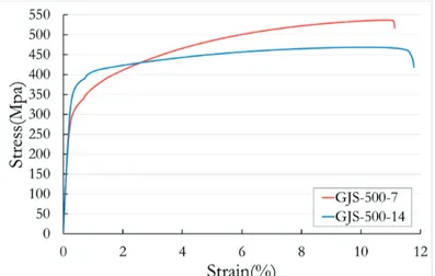
Table 4 shows the tensile properties of the 30mm thick plate for two cast materials. Figure 11 shows typical stress/strain curves of the tensile test for each material. Grade GJS-500-7 showed higher ultimate tensile strength than grade GJS-500-14, which could be due to the presence of pearlite as well as higher nodularity. Lower ultimate tensile strength and ductility of grade GJS-500-14 compared to the standard, could be attributed to the lower nodularity (less than 85%) in this material.

The tensile results has been used as a reference for benchmarking the values obtained from DIC and in-situ tensile test, and also to optimize the material parameters.

Table 4. Tensile properties of the grades GJS-500-14 and GJS-500-7, 30mm thick plate.

Grade _{modulus (GPa)}Elasticity Yield strength _(MPa) Ultimate tensile _{strength (MPa)} Elongation to _{fracture (%)}

GJS-500-7 165±5.5 377±2.7 539±2.5 10.4±0.6

(31)

Figure 11. Typical stress/strain curves of grades GJS-500-7 and GJS-500-14, 30mm thick plate.

3.2 METHOD DEVELOPMENT FOR DIC ANALYSIS (SUPPLEMENT I)

3.2.1 Pit etching reagent

The effect of the two pit etching reagents on the microstructure of the cast material is presented in Figure 12. The pits appeared as dark spots on the micrographs. It has been expected that the pits mostly form on the local defects such as dislocations, vacancies, inclusions and impurities [90, 95].

Reagent B had two distinct disadvantages for DIC pattern generation: (i) sever oxidation of graphite particles due to high amount of hydrogen peroxide, (ii) too small pit size (Figure 12(b)). The former disadvantage would mask the regions around graphite particles and the later would induce errors in displacement and strain measurement. However, these issues were less obvious when using reagent A since the amount of hydrogen peroxide was much lower and the pits were relatively larger (Figure 12(a)). Therefore, reagent A was considered for generating speckle patterns in the rest of the investigations.

Figure 12. The microstructure of the cast material, pit etched with (a) reagent A, (b) reagent B. Images were taken in 63X magnification.

(32)

3.2.2 Optimum subset size and magnification

Table 5 shows the size and distribution of the speckles and the minimum subset size for each pattern group in two magnifications. Note that in the un-etched group, graphite particles (natural microstructure) were considered as speckle pattern. The minimum subset size was calculated based on Eq. (5).

Pit etching provided smaller and denser pattern compared to the un-etched condition (natural microstructure pattern). Higher etching temperature resulted in higher density, smaller NND and smaller Pit size. Nevertheless, pit etching at 75 and 100˚C showed almost the same results. It can be interpreted that temperatures higher than 75˚C had negligible effect on the number and size of pits due to the faster evaporation of the reagent on the surface.

The small standard deviation (SD) of density values indicated a good reliability of pit etching procedure for speckle generation. Figure 13 shows the speckle patterns provided by graphite particles and pit etching at 75˚C with the calculated minimum subset sizes.

Table 5. Size and distribution of the speckles and the minimum subset size calculated for each speckle pattern. Un-etched Pit etched at room temperatu re Pit etched at 50˚C Pit etched at 75˚C Pit etched at 100˚C Mean Radius (µm) 16.5 7.2 3.7 1.7 2.8 1.3 2.7 0.9 2.6 1 Average area (µm2₎ 1089.4 105 48.4 6.2 31.1 5.1 27.5 3.1 26,4 3.4 Nearest neighbor distance (NND) (µm) 48.3 20.3 22.1 10 11.8 3.9 8.6 2.1 7.9 2.6 Density (number/mm²) 81 7 486 29 2405.1 128 5286.1 362 5444 208 Minimum subset size for 15.8X (pixels) 85 85 33 33 19 19 13 13 13 13 Minimum subset size for 63X (pixels) 341 341 133 133 71 71 51 51 51 51

Generated speckles had to be larger than the 3 3 pixel array. The area covered with a 3 3 array of pixels for 15.8X and 63X magnifications were 43.16 and 2.62 µm2_{, respectively. In 63X}

magnification, the average area of speckles for all groups were larger than the limit size (see Table 5). However, in the 15.8X, only natural microstructure pattern and pit etching at room temperature had the average speckle size larger than the limit size, and thus, the rest of the groups were excluded from further investigation.

(33)

Figure 13. (a)&(c) Natural microstructural pattern in un-etched condition, (b)&(d) pit etched pattern at 75 ˚C. The top and bottom images correspond to 15.8X and 63X nominal magnifications, respectively.

The squares that were pointed by the arrows show the minimum subset size calculated for each speckle pattern.

3.2.3 Spatial resolution and standard deviation

Spatial resolution and DIC standard deviation were evaluated by correlating the reference image with one stationary image in the DIC program employing the pattern’s minimum subset sizes. For strain spatial resolution and standard deviation, step size and strain window of 5 pixels and 5 5 data points (VSG = 21 21 pixels), respectively, were used.

Figure 14 shows the measured displacement and strain spatial resolution and standard deviation. It is clear that the displacement and strain were significantly improved by using pit etching pattern compared to the natural microstructural pattern. Similarly, increasing the pit etching temperature has improved the spatial resolution in 63X magnification. This can be attributed to the possibility of the use of smaller subset size.

Displacement spatial resolutions in both magnifications were identical because it only relates to the subset size and pattern characterization. Strain spatial resolution values were smaller in 63X magnification due to the larger field of view. On the other hand, the standard deviation errors in both displacement and strain were increased by using pit etching and pit etching in high temperature. This was due to the fact that the standard deviation error increases by decreasing the subset size [59, 60, 63]. The small error bars for standard deviations demonstrated the good reliability of the produced patterns in DIC measurements.

(34)

Figure 14. Strain and displacement spatial resolution and standard deviation that were obtained by patterns’ minimum subset size

In this study, the pattern with the lowest strain spatial resolution was favourable to enable finer localized strain detection around and in between graphite particles. In this case, pit etching at room temperature and 75˚C showed the best results in 63X and 15.8X magnification, respectively. Consequently, in-situ tensile test was performed on the samples with the above mentioned pit etching procedure and natural microstructural pattern to compare the detection of the local strain and assess the accuracy of the minimum subset size for calculating the elastic modulus.

3.2.4 Validation of the DIC results

Using DIC, the average of full-field strain was measured for every deformed images in the stress range of 50-150MPa (below yield point). The results was used to calculate the elastic modulus of the material, following the regression method. The obtained values were assessed by comparing to standard elastic modulus in the same range of stress. Note that in such stress range, elastic modulus was measured as 151 GPa in the standard tensile test.

As can be seen in Figure 15, the elastic modulus values obtained from DIC conform to standard test results with a good approximation. This was attributed to the correct selection of subset size for each pattern. In addition, this can validate the localized strain values that are measured by this method.

(35)

Figure 15. Comparison between elastic modulus obtained from DIC analysis and standard tensile test.

Although correct elastic modules were obtained for all the patterns,pit etching pattern enabled much better spatial resolution and can be used for determination of strain fields in regions between the graphite particles. This gradient detection was not possible by using natural microstructural pattern. Correspondingly, Figure 16 represents an example of DIC results obtained in 63X magnification for two in-situ tensile test samples with natural microstructural and pit etching pattern in stress level of 150MPa. The use of pits as speckle pattern improved spatial resolution and local gradient detection by making the possibility of using smaller subset size.

Figure 16. Typical DIC strain maps for the micrographs that were captured in stress values close to 150MPa with 63X nominal magnification using: (a) natural microstructural pattern, (b) pit etching at

75˚C.

3.2.1 Speckle pattern on ferritic/pearlitic microstructure

Figure 17 shows ferritic/pearlitic microstructure of GJS-500-7 after applying the pit etching procedure at 75˚C, together with an example of the subset size used for the DIC analysis. Similar to fully ferritic material (GJS-500-14), the pit etching provided a random, dense and

(36)

high contrast pattern in both ferrite and pearlite regions that can be used as speckle pattern for DIC analysis.

Figure 17. The speckle pattern (pits) produced by pit etching procedure in the microstructure of the cast material. The square which is pointed by the arrow indicates the subset size.

3.2.2 Advantages and disadvantages of the pit etching procedure

In addition to enabling higher spatial resolution measurement, the pit etching procedure is cheap and fast without requiring expensive equipment. Furthermore, there would be no debonding between the speckles and surface of the material and the speckles do not mask the underlying microstructural features. The pattern can be applied on delicate samples with different geometries since the samples only need to be heated and immersed in the etching reagent.

However, the etching reagent contains H2O2 and HCl which are hazardous chemicals and need

special precautions before usage. Furthermore, the procedure does not make any speckle pattern in the graphite, which may cause inaccurate strain gradient detections inside the graphite particles. Therefore, the DIC strain maps only can be measured in the matrix and graphite particles smaller than subset size.

3.3 MICROSTRUCTURAL DEFORMATION (SUPLEMENTS III AND IV)

During in-situ tensile test, the microstructural deformation can be characterize as several steps depending on the loading level. In the initial phase of loading, shear bands appear at approximately 45° to the loading direction, which is expected for pure tensile loading (this will be discussed later). By raising the load, decohesion of graphite and ferrite was observed at several locations in the material. Initiation of plastic slip bands in the vicinity of sharp corners of graphite inside the ferrite phase was observed in stress levels slightly higher than the Yield stress of the material. The last type of deformation was propagation of micro-cracks inside the ferrite regions at approximately45° to the loading direction. Crack initiation is thus possibly caused by shear slip bands. Failure occurred almost instantly by joining of the micro-cracks.

3.3.1 Graphite/matrix decohesion

Figure 18 shows a series of micrographs from a typical nodular graphite surrounded by ferrite in four different overall strain levels (load was applied in the x-direction). For these types of

(37)

graphite, increasing load led to a significant increase of decohesion growth of graphite/ferrite in a large area around the nodule. At the structural strain of 7% the maximum amount of decohesion for this graphite was measured to be approximately 11 µm, as indicated by the arrow in Figure 18(d). It should be noted that small black dots inside the ferrite and pearlite are pits, which were used as speckle pattern in DIC measurement.

Figure 18. Decohesion procedure of a nodular graphite embedded in ferrite at overall elongation of : (a) 0%, (b) 0.5% (yield point), (c) 4.5%, and (d) 7% (before failure). The arrow shows the location where

the maximum decohesion happened. Total elongation to failure was 7.6%.

Smaller gap was measured for an irregular shape graphite particle, embedded in ferrite, compared to the nodular graphite, as shown in Figure 19. The gap was measured 9 µm for 7% overall elongation, indicated by the black arrow in Figure 19(d). This smaller gap was likely due to the irregular geometry of the graphite particle, which produced higher mechanical bonding to the matrix. This also resulted in fracture of the graphite particle indicated by the white arrows in Figure 19(d).

Figure 19. Decohesion and internal cracking of an irregular shape graphite embedded in ferrite phase at overall elongation of: (a) 0%, (b) 0.5% (yield point), (c) 4.5%, and (d) 7% (before failure). The black arrow shows the location of maximum decohesion. The white arrows show the internal cracking of

(38)

3.3.2 Micro-crack development inside the matrix

In this thesis a micro-crack is defined as a microstructurally short crack, which develop at the interface between the graphite and the ferrite phases and propagates a distance of some micrometers. In this case, the load is normal or parallel to the micro-crack plane. A relatively large plastic zone ahead of the crack tip compared to the length of the crack often characterizes a micro-crack. These micro-cracks do not necessarily coalesce to form a larger crack.

Figure 20 shows a series of micrographs for an irregular shaped graphite, where the plastic deformation developed slip bands and a micro-crack in a ferrite region. This micro-crack was the earliest which was formed during the deformation. Decohesion of graphite/ferrite formed holes around the graphite particles which acted as stress concentrators and thus promotes micro-crack initiation. Plastic deformation in the ferritic matrix occurs as a result of the stress concentration caused by these holes. Micro-crack forms as the localized plastic deformation exceeds the failure. The combination of these slip bands and micro-cracks (as could be seen by the optical micrograph) is pointed by the arrow in Figure 20(d). To clarify, this region is magnified in Figure 21 with a SEM micrograph which was taken after the failure, indicating graphite decohesion with significant plastic deformation in the ferrite matrix and two micro-cracks (shown by arrows) emanating from the graphite corner.

Figure 20. Formation of slip bands and V-shape micro-crack around an irregular shape graphite embedded in ferrite at overall elongation of: (a) 0%, (b) 0.5% (yield point), (c) 4.5%, and (d) 7% (before

failure). The black arrow indicates the location of micro-crack and slip bands.

The micro-crack initiated in overall stress and strain of 348 MPa and 0.98%, respectively. It was found that the micro-cracks formed a V-shape and were arrested a few micrometers inside the ferrite region before reaching the ferrite/pearlite boundary, see Figure 21. This could be due to the work hardening effect that continuously developed in front of the micro-crack which act as a barrier for further crack propagation and force changes in the direction of propagation. The direction of the propagation was typically about 45˚ to the loading direction, which indicates propagation parallel to plane of maximum shear stress.

(39)

Figure 21. The SEM micrograph of the V-shape micro-crack and slip bands inside the ferrite, taken after the sample failure.

3.4 LOCALISED STRAIN MEASUREMENT (SUPPLEMENT II AND IV)

3.4.1 Strain at the onset of the first micro-crack

Microstructural strains were studied for the micrographs that were taken at the onset of the first micro-crack in the field of view in five different samples. Table 6 shows the local and average strains together with overall stresses and strains. Micro-crack local strain was measured from an average of strain points within an area of 27µm 27µm (50 50 pixels) around the micro-crack. The DIC average strain is the average of strain which was measured across the entire field of view. The overall strains and stresses were measured from the miniature tensile stage data. Note that the strain values were measured in direction parallel to the applied force. The DIC average strain and the overall strain for every Sample are in a good agreement. The discrepancies could be attributed to the limited field of view in the microscope compared to the overall strain that obtained from the whole gage length.

The local strains at the regions of the micro-cracks were much larger than the average strain. This demonstrated that strain concentration occurred at the location of the micro-crack around the graphite particles. The first micro-cracks appeared as the localized strain concentration exceeded 2%.