Energy norm a posteriori error estimates for a continuous/discontinuous Galerkin approximation of the Reissner-Mindlin plate

JTH R

R

2011:05

E

NERGY

N

ORM

A P

OSTERIORI

E

RROR

E

STIMATES FOR A

C

ONTINUOUS

/D

ISCONTINUOUS

G

ALERKIN

A

PPROXIMATION OF THE

R

EISSNER

-M

INDLIN

P

LATE

P

H

M

G. L

_{Department of Mechanical}

Engineering

Jönköping University

SE-551 11 Jönköping

2

_{Department of Mathematics}

and Mathematical Statistics

Umeå University

SE-90187 Umeå

A Survey of High Level Test Generation

Methodologies and Fault Models

Tomas Bengtsson and Shashi Kumar

ISSN 1404 – 0018

Research Report 04:5

D

M

E

J

U

SE-551 11 J

ISSN: 1404-0018

Continuous/Discontinuous Galerkin Approximation of the

Reissner-Mindlin Plate

Peter Hansbo

and Mats G. Larson

1_{Department of Mechanical Engineering, Jönköping University, SE-55111 Jönköping, Sweden}

2_{Department of Mathematics and Mathematical Statistics, Umeå University, SE-90187 Umeå, Sweden}

SUMMARY

We derive energy norm a posteriori error estimates for continuous/discontinuous Galerkin finite element approximations of the Mindlin-Reissner plate model. The finite element method is based on continuous piecewise second degree polynomial approximation for the transverse displacements and the rotated Brezzi-Douglas-Marini approximation, with tangential continuity only, for the rotations. This approximation enjoys optimal convergence, uniformly in the plate thickness. The a posteriori error estimates are residual based and are derived using techniques based on Helmholtz decompositions.

1. INTRODUCTION

An important research area in finite element analysis has been the construction of efficient elements for moderately thick plates modeled by the Reissner-Mindlin plate equation. This model involves the approximation of the transversal displacement and rotation of the mid surface of the plate. The difficulty is that as the plate thickness tends to zero the rotation vector tends to the gradient of the transversal displacement. If the discrete spaces are chosen in such a way that this limit can not be satisfied we may obtain a deterioriation of the approximation known as locking. Several approaches have been proposed to this problem including under-integration and replacement of the gradient of the displacement by a suitable projection. The latter idea, underpins, e.g., the MITC element family of Bathe and co-workers, first introduced in [2], and has been used extensively in the mathematical literature to prove convergence, see, e.g., [1, 7, 13, 20].

In recent work, [15], we proposed using standard continuous piecewise quadratic elements for the transversal displacement together with discontinuous piecewise linear elements for the rotation in combination with a discontinuous Galerkin formulation. Using this approach, there is no need for an independent approximation or projection of the shear stress term since the gradient of the displacement belongs to the space used to approximate the rotations. When the thickness of the plate tends to zero we obtain the Kirchoff plate and our scheme simplifies to the method proposed in [14]. The method can also be directly extended to higher order polynomials. In [15] a priori error estimates that are uniform in the plate thickness as well as duality– based a posteriori error estimates are presented. A related method, using fully discontinuous

approximations for both displacements and rotations, was considered by Bösing, Madureira, and Mozolevski [6].

Since the gradient of continuous piecewise quadratic polynomials is tangentially continuous, it follows directly from the analysis in [15] that it is indeed possible to use tangentially continuous edge elements for the rotations, instead of the larger space of discontinuous piecewise linears, and still maintain optimal convergence uniformly in the plate thickness.

In this contribution we derive energy norm a posteriori error estimates for the new method based on linear edge elements for the rotations and continuous piecewise quadratics for the displacement. The estimates are of residual type and can be used as a basis for an adaptive algorithm. We derive the estimates using Helmholtz decomposition techniques. Related work include the a posteriori error estimates for discontinuous Galerkin approximations of the Poisson equation and the elasticity system [3, 18], for continuous/discontinuous Galerkin [17] and nonconforming Morley [4] approximations of the Kirchoff-Love plate, and for different types of conforming, nonconforming, and stabilized Reissner-Mindlin elements by Carstensen and co-workers [?, 11].

The reminder of the paper is organized as follows: In Section 2 we introduce the Reissner-Mindlin plate model, In Section 3 we formulate the finite element method, in Section 4 we formulate and prove the a posteriori error estimate, and finally in Section 5 we present some illustrating numerical examples.

2. THE REISSNER-MINDLIN PLATE MODEL 2.1. The Reissner-Mindlin equations

We consider a plate of constant thickness t with midsurface that occupies a polygonal domain

Ω_{in R}2_{. The Reissner-Mindlin plate model with clamped boundary conditions takes the form:}

find the transversal displacement u :Ω→ R, the rotation θ :Ω→ R2of the median surface, and the shear stress ζ :Ω→ R2such that

−div ζ = g inΩ_{, (1)} −divσ(θ) + ζ = 0 inΩ_{, (2)} ζ − κ t2(∇u − θ) = 0 inΩ, (3) θ = 0 on ∂Ω, (4) u =0 on ∂Ω_{. (5)}

Here g is the transverse surface load and

ε(θ) = (Grad θ + (Grad θ)T)/2, σ(θ) = 2µε(θ) + λ(div θ)I (6)

are the 2 × 2 strain and stress tensors. Here,

Grad θ =      ∂θ1 ∂x1 ∂θ1 ∂x2 ∂θ2 ∂x1 ∂θ2 ∂x2      , div σ =' ∂σ11 ∂x1 +∂σ12 ∂x2 ,∂σ21 ∂x1 +∂σ22 ∂x2 ( .

The material constants are given by the relations κ = E k/(2(1 + ν)), µ := E/(6(1 + ν)), and λ := νE/(12(1 − ν2)), where E and ν are the Young’s modulus and Poisson’s ratio, respectively, and k ≈ 5/6 is a shear correction factor.

2.2. Variational formulation

Eliminating the shear stress, the transverse displacement and rotation vector are solutions to the following variational problem: find (u, θ) ∈ H₀1(Ω_{) × [H}1

0(Ω)] 2_{such that} a(θ,ϑ) + κ t2(∇u − θ,∇v − ϑ) = (g, v), ∀(v, ϑ) ∈ H 1 0(Ω) × [H10(Ω)]2, (7)

where the bilinear form is defined by

a(θ,ϑ) = (σ(θ),ε(ϑ)). (8)

Here and below (·, ·) denotes the standard L2(Ω_{) inner product for scalar, vector, and tensor}

valued functions.

3. THE CONTINUOUS/DISCONTINUOUS FINITE ELEMENT METHOD 3.1. Finite element spaces

Let T = {T} denote a subdivision of Ω _{into a geometrically conforming finite element mesh}

with shape regular elements T of diameter hT. We shall use continuous piecewise quadratic polynomial approximation of the transverse displacement

Vh={v ∈ H01(Ω) ∩ C0(Ω) : v|T∈P2(T) for all T ∈ T } (9) and piecewise linear edge element approximations of the rotations

W_{h:= {ϑ ∈ H0(rot;}Ω_{) : ϑ|T}∈[P1(T)]2for all T ∈ T }. (10)

Remark 3.1. With this choice of spaces the following inclusion holds

∇Vh⊂ Wh. (11)

Thus, in the limit t →0, gradients of functions in Vh belong to Wh, which retains enough approximation power to allow optimal order convergence. We note that in fact the gradient of the continuous piecewise quadratics is exactly the kernel of the rotation operator acting on the edge elements.

Remark 3.2. In previous work, [15], we considered completely discontinuous rotations, the

convergence proof of which carries over to the present case with minor modifications. The advantage of the present approximation is obvious, however: since the ratio of edgesE to triangles T in a mesh is approximately3:2, we exchange 6T degrees of freedom (in the fully discontinuous case) for 2E ≈ 3T degrees of freedom, effectively halving the number of rotational unknowns without affecting the convergence rate.

3.2. The finite element method

To define the finite element method we introduce the set of edges in the mesh, E = {E}, and we split E into two disjoint subsets

E= EI∪ EB,

where EI is the set of edges in the interior ofΩ and EB is the set of edges on the boundary. Further, with each edge we associate a fixed unit normal n such that for edges on the boundary n is the exterior unit normal. We denote the jump of a function v ∈Γ_{hat an edge E by [v] = v}+− v− for E ∈ EI and [v] = v+for E ∈ EB, and the average 〈v〉 = (v++ v−)/2 for E ∈ EI and 〈v〉 = v+for E ∈ EB, where v±=lim'↓0v(x ∓ ' n) with x ∈ E. In some instances, we shall use the unit outward pointing normal to T, which we denote by nT.

For later use, we introduce weak interpolation operators

π : L2(Ω) → Vh, πBDM: [H1(Ω)]2→ Wh,

where π is of Scott-Zhang type and πBDMis the edge element (rotated Brezzi-Douglas-Marini)

interpolation operator with the following properties: [t · πBDMϑ] = 0, /ϑ − πBDMϑ/Hm_(T) ≤ Chk+1−m T /ϑ/Hk+1_(T) m =0, 1, /∇ ·(ϑ − πBDMϑ)/Hm_(T) ≤ Chk−m T /∇ ·ϑ/Hk_(T), m =0, 1, (12)

for all ϑ ∈ Hk+1(T). Here, t denotes the tangent vector on each edge E such that if n = (nx, ny),

t =(ny, −nx). For the Scott-Zhang interpolant, we recall the following interpolation inequalities /v − πv/Hm_(T)≤Chs

T|v|Hs_{(N (T))}, 0 ≤ m ≤ s ≤ 3 (13)

where N (T) is the domain associated with T and the elements sharing nodes with T. Our method can be formulated as follows: find (U,Θ) ∈ Vh× Whsuch that

ah(Θ, ϑ) + κ

t2(∇U −Θ, ∇v − ϑ) = (g, v) ∀(v, ϑ) ∈ Vh× Wh (14)

with the bilinear form a_h(·, ·) defined by ah(Θ, ϑ) = ) T∈T (σ(Θ_{), ε(ϑ))T} (15) − ) E∈EI∪EB (〈n · σ(Θ_{)〉, [ϑ])E}+(〈n · σ(ϑ)〉,[Θ_])E +(µ + λ) γ) E∈E (h−1_E [Θ_{], [ϑ])E.}

Here γ is a positive constant (for the requirement of which, cf. [15]) and hEis defined by hE=*|T+| + |T−|+ /(2|E|) for E = ∂T+∩ ∂T−,

with |T| the area of T, on each edge. Furthermore, (·, ·)ω denotes the standard L2(ω) inner product for scalar, vector, and tensor valued functions.

The approximation of the shear stress is defined, elementwise, by direct evaluation

Z|_T= κ t2(∇U −Θ) , , , ,_T .

Lemma 3.3. The method(14) is consistent in the sense that ah(θ −Θ, ϑ) +

κ

t2(∇u − ∇U − (θ −Θ), ∇v − ϑ) = 0, (16)

for all ϑ ∈ Whandv ∈ Vh.

4. THE ENERGY NORM A POSTERIORI ERROR ESTIMATE 4.1. Helmholtz decompositions

We shall use a variant of the Helmholtz decomposition of 2 × 2 tensor fields introduced in [4]. In the following we shall use the following definitions: the curl of a scalar function

rot_v:=' ∂v ∂x2 , −∂v ∂x1 ( , and the curl of a vector

rot v =∂v2 ∂x1

−∂v1 ∂x2

, so that by Green’s formula

(rot v, w)Ω=(v, ∇w)Ω+(t · v, w)∂Ω, and

(rot w, v)Ω=(w, rot v)Ω−(t · v, w)∂Ω.

Lemma 4.1. Let χ ∈ L2(Ω_{, R}2×2_{) be a symmetric second order tensor field. Then the following}

decompositions hold:

A: There exist ψ ∈ [H₀1(Ω_)]2_{and φ ∈ [H}1

0(Ω)]2such that χ = σ(ψ) + Rot φ, where Rot φ =      −∂φ1 ∂x2 ∂φ1 ∂x1 −∂φ2 ∂x2 ∂φ2 ∂x1     

is a symmetric2 × 2 matrix, and ψ satisfies the equation

a(ψ, v) = (χ,Grad v), ∀v ∈[H1(Ω_)]2_{. (17)}

Furthermore, the following stability estimate holds

/ψ/1+ /φ/1≤C/χ/. (18)

We also note that

div Rot φ = 0. (19)

B: There exist α,β ∈ H2₀(Ω_{) such that}

and

χ = σ(∇α) + σ(rot β) + Rot φ. (21)

Furthermore, α and β satisfy the equations

a(∇α,∇v) = (div div χ, v), ∀v ∈ H2₀(Ω_{), (22)}

a(rot β,rot v) = (rot div χ, v), ∀v ∈ H₀2(Ω_{), (23)}

and the following stability estimate holds

/α/2+ /β/2+ /γ/1≤C/χ/. (24)

PROOF_{. We want to combine the problems}

a(∇α,∇v) = (div div χ, v) = −(div χ,∇v) = (χ,Grad ∇v) (25) and

a(rot β,rot w) = (rot div χ, w) = −(div χ,rot w) = (χ,Grad rot w) (26) to arrive at (17). We have tr(ε(rot u)) = 0 and, using Green’s formula, we then get

(ε(rot u),ε(∇v)) = −(rot u, div ε(∇v))

= −(u, rot div ε(∇v)) = 0, ∀u, v ∈ H2₀(Ω_),

(27)

and thus

a(rot u, ∇v) = 0, ∀u, v ∈ H2₀(Ω). (28) We may thus conclude that

a(∇α + rot β,∇v + rot w) = (χ,Grad (∇v + rot w)), ∀v, w ∈ H₀2(Ω_{). (29)}

Further, using the fact that any z ∈ [H1₀(Ω_)]2 _{may be written in the form z = ∇v + rot w with}

v, w ∈ H₀2(Ω_{) it follows that}

a(∇α + rot β, z) = (χ,Grad z), ∀z ∈H1₀(Ω_{), (30)}

and by the symmetry of the stress tensor

(χ,Grad z) = (σ(∇α + rot β),ε(z)) = (σ(∇α + rot β),Grad z), (31) or

(−div (σ(∇α + rot β) − χ), z) = 0, (32)

from which it follows that, in the sense of distributions,

div_{(χ − σ(∇α + rot β)) = 0.} (33)

Thus there exists φ such that

χ − σ(∇α + rot β) = Rot φ. (34)

4.2. Preliminaries

We shall need the following technical result in the proof of the a posteriori error estimate. We let H(div;Ω_{) = {η ∈ L}2₍Ω_{, R}2×2_{) | /div η/}2_{< ∞}be the space of 2 × 2 tensor fields which together}

with their divergence belong to L2(Ω_{). Then the estimate}

) T ([v], n · η) ≤ C -) E⊂∂T h−1_E /[v]/2_E .1/2 -) T∈T /η/2_T+h2_T/div η/2_T .1/2 (35)

holds for all v ∈ Whand η ∈ H(div;Ω). A detailed proof is included in Larson and Målqvist [19]. Here and below, C denotes a generic constant independent of the meshsize, not necessarily the same at different instances.

We shall make frequent use of the following inequalities: the inverse inequality

/h1/2_T 〈n ·σ(ϑ)〉/2_∂T≤C/σ(ϑ)/2_T ∀ϑ ∈ [P1(T)]2, (36)

which is proved by scaling and finite dimensionality; the trace inequality /v/2_∂T≤C*h−1 T /v/ 2 T+hT/∇v/2T + ∀v ∈ H1(T), (37)

(for proofs of these inequalities, cf. Thomée [21]); and finally

/n · v/_∂T,−1/2≤C(/v/T+hT/div v/T) ∀v ∈H(div; T), (38) proven in [19].

4.3. The a posteriori error estimate

We are now ready to formulate our main result. We introduce the following norm |/(v, θ)/|2= )

T∈T

(σ(θ), ε(θ))_T+t−2(∇v − θ,∇v − θ). (39)

Theorem 4.2. The following a posteriori error estimate holds:

|/(u − U, θ −Θ_)/|2≤C ) T∈T

η2_T, (40)

where the element indicator ηTis defined by

η2_T=h2_T(h2_T+t2)/g − div Z/2_T+hT(h2T+t 2_)/n T·[Z]/2∂T (41) +h2_T/divσ(Θ_{) − Z/}2 T+hT/nT·[σ(Θ)]/ 2 ∂T +h−1_E /[Θ]/2_∂T.

PROOF. For brevity we let eu =u − U, eθ =θ −Θ, and eζ =ζ − Z denote the errors in

applied derivatives we obtain |/(eu, eθ)/|2=

)

T∈T

(σ(eθ), ε(eθ))T+(eζ, ∇eu− eθ)T

= ) T∈T (ε(eθ), σ(ψ))T−(eζ, ψ)T + ) T∈T (eζ, (∇eu− eθ) − (∇α − ψ))T + ) T∈T (eζ, ∇α)T + ) T∈T (ε(eθ), Rot φ)T =I + I I + I I I + IV. We proceed with estimates of the four terms.

TermI . _{For the first term I we first eliminate the exact solution u using equation (7) and the}

fact that ψ ∈ [H1₀(Ω)]2. Then we use the definition of the finite element method (14) to subtract the edge interpolant πBDMψ as follows

I = ) T∈T (ε(eθ), σ(ψ))T−(eζ, ψ)T = − ) T∈T (σ(Θ_{), ε(ψ))T}+(Z, ψ)T = − ) T∈T (σ(Θ_{), ε(ψ − πBDMψ))T+(Z, ψ − πBDMψ)T} −) E∈E (〈n · σ(Θ_{)〉, [πBDMψ])E+([}Θ_{], 〈n · σ(πBDMψ)〉)E} +) E∈E γh−1_E([Θ_{], [πBDMψ])E}. Next using Green’s formula together with the identity

[n · σ(Θ_{) · (ψ − πBDMψ)] + 〈n · σ(}Θ_{)〉 · [πBDMψ]} =[n · σ(Θ_{) · (ψ − πBDMψ)] − 〈n · σ(}Θ_{)〉 · [ψ − πBDMψ]} =[n · σ(Θ_{)] · 〈ψ − πBDMψ〉,} we arrive at I = ) T∈T (∇ · σ(Θ_{) + Z, ψ − πBDMψ)T} (42) −) E∈E ([n · σ(Θ_{)], 〈ψ − πBDMψ〉)E} −) E∈E ([Θ_{], 〈n · σ(πBDMψ)〉)E} +) E∈E γh−1_E ([Θ_{], [πBDMψ])E} =I1+I2+I3+I4. (43)

These four terms may now be directly estimated in a straightforward manner using the Cauchy-Schwartz inequality, the trace inequality (37), the inverse inequality (36), the

interpolation error estimates (12) and (13), and finally the stability estimate (18). For convenience we include the estimates.

TermI1. Using the Cauchy-Schwartz inequality on the sum and scaling with suitable powers of

hT we obtain I1= ) T∈T (∇ · σ(Θ_{) + Z, ψ − πBDMψ)T} ≤ -) T∈T h2_T/∇ ·σ(Θ_{) + Z/}2 T .1/2 -) T∈T h−2_T /ψ − πBDMψ/2T .1/2 .

Next using the interpolation error estimate (12) and the stability estimate (18) we have )

T∈T

h−2_T /ψ − πBDMψ/2T≤ /ψ/1≤ /eθ/1

TermI2. Using the Cauchy-Schwartz inequality on the sum with suitable scaling we get

I2= − ) E∈E ([n · σ(Θ_{)], 〈ψ − πBDMψ〉)E} ≤ -) E∈E hT/[n · σ(Θ)]/2E .1/2 -) E∈E h−1_T /〈ψ − πBDMψ〉/2E .1/2 .

Using the trace inequality (37) followed by the interpolation error estimate (12) and the stability estimate (18) we have ) E∈E h−1_T /〈ψ − πBDMψ〉/2E≤ ) T∈T / h−2_T /ψ − πBDMψ/2T+ /ψ − πBDMψ/2T,1 0 ≤C/ψ/2₁.

TermI3. Using the Cauchy-Schwartz inequality on the sum with suitable scaling we get

I3= − ) E∈E ([Θ_{], 〈n · σ(πBDMψ)〉)E} ≤ -) E∈E h−1_E /[Θ_]/2 E .1/2 -) E∈E hE/〈n ·σ(πBDMψ)〉/2E .1/2 .

Using the inverse inequality and the stability of the interpolation operator πBDMwe have

) E∈E hE/〈n ·σ(πBDMψ)〉/2E≤C ) T∈T /σ(πBDMψ)/2T≤C/ψ/21.

TermI4. Using the Cauchy-Schwartz inequality on the sum with suitable scaling we get

I4= ) E∈E γh−1_E ([Θ_{], [πBDMψ])E} ≤ -) E∈E γh−1_E /[Θ_]/2 .1/2 -) E∈E h−1_E /[πBDMψ]/2E .1/2

Using that [πBDMψ] = [πBDMψ − ψ] since ψ ∈ [H01(Ω)]2, the trace inequality, and the

interpolation estimate we obtain ) E∈E h−1_E /[πBDMψ]/2E≤C ) T∈T / h−2_T /ψ − πBDMψ/2T+ /ψ − πBDMψ/2T,1 0 ≤C/ψ/21.

Collecting the estimates of I1–I4and using the stability estimate (18) we finally get

I ≤ C -) T∈T η2_T .1/2 /ψ/1≤C -) T∈T η2_T .1/2 |/e/|. (44)

TermI I . _{Recalling the following Helmholtz decompositions} e_{θ= ∇αe} θ+ rot βeθ ψ = ∇αψ+ rot βψ we obtain I I =(e_ζ, (∇eu− eθ) − (∇αψ−ψ)) =(eζ, ∇(eu− αe_θ)) + (eζ, rot (βψ− βe_θ)) =I I1+I I2.

TermI I1.We begin by using Galerkin orthogonality, Lemma 3.3, with ϑ = 0 and v = π(eu− αe_θ).

Then, using Green’s formula followed by standard estimates and the interpolation error estimate (13), we obtain I I1=(eζ, ∇((eu− αe_θ) − π(eu− αe_θ))) = ) T∈T (g − div Z, (eu− αe_θ) − π(eu− αe_θ))T +([n · Z]/2, (eu− αe_θ) − π(eu− αe_θ))∂T ≤ ) T∈T C*h2 T/g −div Z/ 2 T+hT/nT·[Z]/2∂T/2 +1/2 /∇(eu− αe_θ)/N(T) ≤C -) T∈T h2_T/g −div Z/2_T+hT/nT·[Z]/2∂T/2 .1/2 /∇(eu− αe_θ)/. (45)

Next we note that

/∇(eu− αe_θ)/2≤ /∇(eu− αe_θ)/2+ /rot βe_θ/2

= /∇eu−(∇αe_θ+ rot βe_θ)/2−2(∇eu, rot βe_θ)

= /∇eu− eθ/2

=t4/eζ/2, (46)

where in the second step we used that eθ= ∇αe_θ+ rot βe_θ is an L2-orthogonal decomposition

and in the third that

(∇eu, rot βe_θ) = ) T∈T (rot ∇eu, βe_θ)T− ) E∈E ([t · ∇eu], βe_θ)E=0.

Finally, combining (45) and (46) we arrive at the following estimate

I I1≤C -) T∈T h2_Tt2/g −div Z/2_T+hTt2/nT·[Z]/2_∂T/2 .1/2 t/eζ/. (47)

TermI I2.Introducing the dual problem: find ϕ :Ω→ Rsuch that

rot div σ(rot ϕ) = −rot rot βe_ζ inΩ, (48)

Using the Lax-Milgram Lemma we conclude that this problem is uniquely solvable and that the stability estimate

/ϕ/2≤C/rot rot βe_ζ/−2=C/rot eζ/−2≤C/eζ/ (50)

holds. Multiplying (48) by βψ− βe_θ and using Green’s formula we obtain

I I2=(rot βe_ζ, rot (βψ− βe_θ)) =(div σ(rot ϕ),ψ − eθ) = − ) T∈T (σ(rot ϕ),ε(ψ − eθ))T + ) T∈T (nT·σ(rot ϕ), ψ − eθ)∂T

According to Lemma 4.1 (with χ := σ(eθ)), there exists φ such that

(σ(rot ϕ),ε(ψ − eθ))T = (ε(rot ϕ),σ(ψ − eθ))T = −(ε(rot ϕ),Rot φ)T = −(Grad (rot ϕ),Rot φ)T

= (rot ϕ,div Rot φ)T−(rot ϕ, nT· Rotφ)∂T,

where we used the symmetry of Rot φ. The first term on the right-hand side vanishes due to (19) and the second upon summation over all elements. Thus we are left with

I I2= ) T∈T (nT·σ(rot ϕ), ψ − eθ)∂T = ) E∈E (n · σ(rot ϕ),[Θ])E = ) E∈E (n · σ(rot ϕ),[t ·Θ_])E =0.

Here we derived the last two equalities as follows. First, using the definition of the dual problem (48) together with the identity rot βe_ζ= div(βe_ζS), where

S = 1 0 1 −1 0 2 , we conclude that σ(rot ϕ) = βe_ζS. Therefore

n · σ(rot ϕ) = (n · S)βe_ζ= tβe_ζ (51)

and thus

(n · σ(rot ϕ),[Θ_])E=(n · σ(rot ϕ),[t ·Θ_])E=0.

TermI I I . _{Using Galerkin orthogonality, Lemma 3.3, we have} I I I = ) T∈T (e_ζ, ∇(αψ− παψ))T (52) = ) T∈T (g − ∇ · Z, αψ− παψ)T+([n · Z]/2, αψ− παψ)∂T (53)

Again using standard estimates and the interpolation inequality (13) we get

I I I ≤ -) T∈T h4_T/g −div Z/2_T+h3_T/n_T·[Z]/2/2_∂T .1/2 /αψ/2 ≤ -) T∈T h4_T/g −div Z/2_T+h3_T/nT·[Z]/2/2_∂T .1/2 /eθ/,

where we used the stability estimate (24) in the last inequality.

TermI V . _{To estimate the fourth term IV we first use Green’s formula to conclude that}

IV = ) T∈T (ε(eθ), Rot φ)T = ) T∈T (Grad (eθ), Rot φ)T = ) E∈E ([Θ_{], n · Rot φ)E},

where again we used symmetry and (19). Next we note that we can write the right side in the following form IV = ) E∈E ([Θ_{], n · Rot φ)E} = ) T∈T (Θ_{− w, nT}· Rotφ)∂T (54)

for any continuous function w which is zero on the boundary ∂Ω_{. We can now estimate the}

contributions from each triangle as follows

(Θ_{− w, nT}· Rotφ)∂T≤ /Θ− w/∂T,1/2/nT· Rotφ/∂T,−1/2 (55) Next using the normal trace inequality (38) with v = rot φi for i = 1, 2, and the fact that div rot φi=0, we obtain the inequality

/n_T· Rotφ/∂T,−1/2≤C/Rot φ/T (56)

which together with (54) and (55) give

IV ≤ C -) T∈T /Θ− w/2 ∂T,1/2 .1/2 -) T∈T /Rotφ/2_T .1/2 ≤C -) T∈T /Θ− w/2_∂T,1/2 .1/2 |/e/|.

Finally, the following inequality, see Larson and Målqvist [19] for a detailed proof, holds inf w∈[C(Ω)]2 ) T∈T /Θ− w/2_∂T,1/2≤C ) T∈T h−1_T /[Θ_]/2 ∂T, (57)

and thus we finally obtain the estimate IV ≤ C -) T∈T h−1_T /[Θ_]/2 ∂T .1/2 |/e/|. (58)

Collecting the estimates of terms I–IV the theorem follows.

5. NUMERICAL EXAMPLES

5.1. Remarks on the implementation of the edge element

The linear edge element is defined in the mathematical literature using degrees of freedom corresponding to weighted integrals of the tangential part of the shape functions along the edge (constant and linear weights), so that the tangential jump of the vectorial shape functions is orthogonal to affine functions on each edge, cf. [8]. In computational electro–magnetics texts, the shape functions are instead typically defined using the Lagrangian basis and its gradients (Whitney elements), cf. [5].

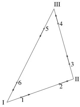
Perhaps, however, the simplest way to implement the linear edge element in practice is to go from integrated quantities to point quantities. If we associate the tangential degrees of freedom with the Gauss points on each edge, we implicitly obtain the desired orthogonality requirements: a shape function that takes the tangential value 1 in one Gauss point and zero in all the others will, since two Gauss points exactly integrates quadratic polynomials along a line, by definition lead to zero integrated (affinely weighted) tangential jump. Using point values we still have the question of wether to establish the shape functions on a reference element, in which case we must use the Piola vector transformation to the physical element, cf. [8], or to work directly on the physical element. We opine that it is more direct to work in physical coordinates. Consider thus the physical element in Fig. 1, with corner nodes locally numbered I–III and edge nodes locally numbered 1–6. To each element is associated a positive orientation of the local node numbering, counterclockwise. Each edge in the mesh is also designated a direction which is assumed positive from the lower global corner node number to the higher. To each side of each element is associated a sign: positive if the local orientation agrees with the direction of the edge associated with the element side, negative otherwise. This sign makes the direction of the shape functions agree across element borders and allows us to work with a default counter clockwise direction, indicated in Fig. 1.

Computing the vectorial shape functions is now straightforward. Denoting the tangential vectors for the edges by ti, where t1=(xII− xI)/|xII− xI|, etc., we can compute the first shape

vector ϕ1by making the ansatz

ϕ₁=(a1+a2x + a3y, a4+a5x + a6y)

and determining the parameters a1–a6by requiring

ϕ₁(x1) · t1= ±1 (sign depending on the positive direction),

ϕ₁(x2) · t1=0,

ϕ₁(x2k−1) · tk=0 and ϕ1(x2k) · tk=0 for 2 ≤ k ≤ 3, and similarly for the remaining five shape functions.

5.2. Accuracy with respect to plate thickness

We consider the exact solution to a clamped Reissner–Mindlin plate on the unit square presented by Chinosi, Lovadina, and Marini [12]. They suggested a right-hand side

g = E 12(1 − ν2₎(12x2(x2−1)(5x 2 1−5x1+1)(2x22(x2−1)2+x1(x1−1)(5x22−5x2+1))+ 12x1(x1−1)(5x22−5x2+1)(2x21(x1−1)2+x2(x2−1)(5x21−5x1+1))), leading to u = u0+ur, where u0= 1 3x 3 1(x1−1)3x32(x2−1)3 and ur= 2t2 5(1 − ν)(x 3 2(x2−1)3x1(x1−1)(5x21−5x1+1) + x31(x1−1)3x2(x2−1)(5x22−5x2+1)), and rotations θ1=(x32(x2−1)3x21(x1−1)2(2x1−1)), θ2=(x31(x1−1)3x22(x2−1)2(2x2−1)).

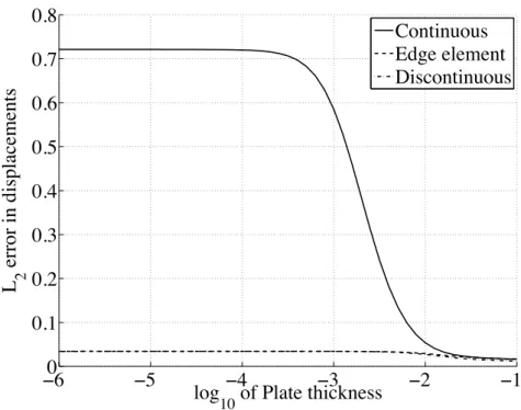
We show, on a fixed mesh, the effect of varying the plate thickness on the L2 error of the

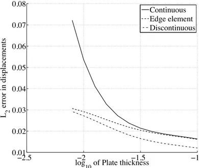
displacements. In Figure 2, we show three different affine approximations of the rotations in combination with a P2 displacement filed: continuous rotations, edge element rotations, and completely discontinuous rotations. We note that only the continuous field locks. In Figure 3 we show the effect at the thicker end of Figure 2. The completely discontinuous field lead to a slight improvement in accuracy compared to the edge element.

5.3. Adaptive refinement and effectivity index

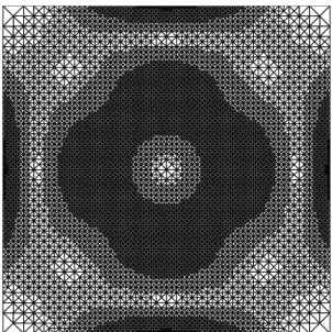
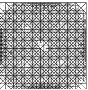
Considering the same problem as previously, we show the variation of the effectivity index, defined as EFF:= 3 C4 T∈T η2T |/(u − U, θ −Θ_)/|

where we arbitrarily set C = 30, on a sequence of meshes in Figure 4, for t = 0.1. This example serves to show that EFFremains fairly constant during the adaptive process. The final adapted meshes given in Figure 5.

The effectivity index is not completely independent on the solution, as can be seen in Figure 6, where the same constant, C = 30, was used. The resulting effectivity index is slightly higher. Note that the degrees of freedom are much more evenly distributed for the thinner plate as a result of increased smoothness of the solution.

REFERENCES

1. Arnold, D.N. Falk, R.S.: A uniformly accurate finite-element method for the Reissner-Mindlin plate. SIAM J. Numer. Anal. 26, 1276–1290 (1989)

2. Bathe, K.J., Dvorkin, E.N.: A four-node plate bending element based on Mindlin-Reissner plate theory and mixed interpolation, Internat. J. Numer. Methods Eng. 21, 367–383 (1985)

3. Becker, R., Hansbo, P., Larson, M.G.: Energy norm a posteriori error estimation for discontinuous Galerkin methods, Comput. Methods Appl. Mech. Engrg. 192, 723–733 (2003)

4. Beirão da Veiga, L., Niiranen, J., Stenberg R.: A posteriori error estimates for the Morley plate bending element. Numer. Math. 106, 65–179 (2007)

5. Bondeson, A., Rylander, T., Ingelström, P.: Computational Electromagnetics, Springer, New York, 2010

6. Bösing, P., Madureira, A.L., Mozolevski, I.: A new interior penalty discontinuous Galerkin method for the Reissner-Mindlin model, Math. Models Methods Appl. Sci. 20, 1343–1361 (2010)

7. Brezzi, F., Fortin, M.: Mixed and Hybrid Finite Element Methods, Springer, New York, 1991

8. Brezzi, F., Fortin, M., Stenberg, R.: Error analysis of mixed-interpolated elements for Reissner-Mindlin plates. Math. Models Methods Appl. Sci. 1, 125–151 (1991)

9. Carstensen, C.: Residual-based a posteriori error estimate for a nonconforming Reissner–Mindlin plate finite element method. SIAM J. Numer. Anal. 39, 2034–2044 (2002)

10. Carstensen, C., Schöberl, J.: Residual-based a posteriori error estimate for a mixed Reissner–Mindlin plate finite element method. Numer. Math. 103, 225–250 (2006)

11. Carstensen, C., Hu, J.: A posteriori error analysis for conforming MITC elements for Reissner–Mindlin plates. Math. Comp. 77, 611–632 (2008)

12. Chinosi C., Lovadina C., Marini L.D.: Nonconforming locking-free finite elements for Reissner-Mindlin plates. Comput. Methods Appl. Mech. Engrg. 195, 3448–3460 (2006)

13. Duran R.,Liberman, E.: On mixed finite-element methods for the Reissner-Mindlin plate model. Math. Comp. 58, 561–573 (1992)

14. Engel, G., Garikipati, K., Hughes, T.J.R., Larson, M.G., Mazzei, L., Taylor, R.L.: Continuous/discontinuous finite element approximations of fourth-order elliptic problems in structural and continuum mechanics with applications to thin beams and plates, and strain gradient elasticity. Comput. Methods Appl. Mech. Engrg. 191, 3669–3750 (2002)

15. Hansbo, P., Heintz, D., Larson, M.G.: A finite element method with discontinuous rotations for the Mindlin– Reissner plate model. Comput. Methods Appl. Mech. Engrg. 200, 638–648 (2011)

16. Hansbo, P., Larson, M.G.: A discontinuous Galerkin method for the plate equation. Calcolo 39, 41–59 (2002) 17. Hansbo, P., Larson, M.G.: A posteriori error estimates for continuous/discontinuous Galerkin approximations of

the Kirchhoff-Love plate. Comput. Methods Appl. Mech. Engrg. 200, 3289–3295 (2011)

18. Hansbo, P., Larson, M.G.: Energy norm a posteriori error estimates for discontinuous Galerkin approximations of the linear elasticity problem. Comput. Methods Appl. Mech. Engrg. 200, 3026–3030 (2011)

19. Larson, M.G., Målqvist, A.: A posteriori error estimates for mixed finite element approximations of elliptic problems. Numer. Math., 108, 487–500 (2008)

20. Pitkäranta, J.: Analysis of some low-order finite-element schemes for Mindlin-Reissner and Kirchhoff plates. Numer. Math. 53, 237–254 (1988)

1

2

3

4

5

6

I

II

III

−6

0

−5

−4

−3

−2

−1

0.1

0.2

0.3

0.4

0.5

0.6

0.7

0.8

L

error in displacements

log

of Plate thickness

Continuous

Edge element

Discontinuous

−2.5

−2

−1.5

−1

0.01

0.02

0.03

0.04

0.05

0.06

0.07

0.08

L

error in displacements

log

of Plate thickness

Continuous

Edge element

Discontinuous

Figure 3. Tail end of Figure 2.

0

5

10

15

20

0

0.5

1

1.5

2

2.5

Refinement level

Effectivity index

0

5

10

15

20

0

0.5

1

1.5

2

2.5

3

3.5

Refinement level

Effectivity index

Figure 6. Effectivity index, t = 10−5.