Use of the Manning Equation for Predicting the Discharge of
High-Gradient Canals and Natural Streams
Ashley A. Ostraff, Steven H. Emerman1, Nicholas D. Udy, Sarah M. Allen, Henintsoa Rakotoarisaona, Janelle Gherasim, Alison M. Stallings, Jeremy N. Saldivar, Kenneth L. Larsen, and Morgan Abbott
Department of Earth Science, Utah Valley University, Orem, Utah
Abstract. The Manning Equation is used to predict stream or canal discharge from hydraulic
radius, slope of the water surface, and a Manning roughness coefficient. Jarrett (1984) proposed that, for high-gradient streams (S > 0.002), the Manning roughness coefficient could be predicted from the hydraulic radius and the slope alone. The objective of this study was to develop separate empirical formulae, depending upon climate and stream bank lithology, for predicting the Manning roughness coefficient for high-gradient canals and natural streams from hydraulic radius and slope. The objective was addressed by separating the database used by Jarrett (1984) according to stream bank lithology, and by carrying out new measurements of the Manning roughness coefficient at nine gradient stream sites with crystalline (igneous and metamorphic) banks and two high-gradient stream sites with carbonate banks in Haiti, nine high-high-gradient stream sites with carbonate banks in Utah, and 14 high-gradient canals in Utah. The data were used to develop empirical formulae for predicting the Manning roughness coefficient for (1) continental climate, clastic stream bank (2) tropical climate, crystalline stream bank (3) continental/tropical climate, carbonate stream bank (4) continental climate, earthen canal with grassy bank. The Manning roughness coefficient was a negative function of hydraulic radius for the first case and a positive function for the other cases, suggesting that the increase in turbulent resistance is caused by the roughness of the sediment in the first case, but by the increase in the Reynolds number, which is proportional to the depth, in the other cases.
1. Introduction
In the absence of a gaging station, flume, or weir, the discharge of a canal or natural stream is often predicted using the Manning Equation
𝑣 =1.49𝑅(/*𝑆,/(
𝑛 (1)
where v is average velocity (ft/s), R is hydraulic radius (ft), S is the slope of the water surface, and n is the Manning roughness coefficient (Dingman 2009). For streams whose width is much greater than the depth, the hydraulic radius is approximately equal to the average depth. Numerous studies have been devoted to the development of methodology for predicting the Manning roughness coefficient, including visual comparison with
1Department of Earth Science
Utah Valley University Orem, Utah 84058 Tel: (801) 863-6864 E-mail: StevenE@uvu.edu
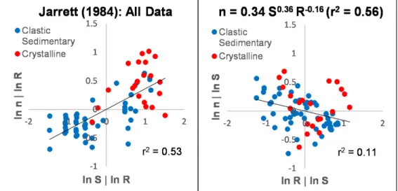
photographs of streams for which n has been measured (Arcement and Schneider 1989), tables of n for streams of various types and materials (Chow 1959), formulae that take into account various aspects of resistance (Arcement and Schneider 1989), formulae that compute n from sediment grain size and hydraulic radius (Bathurst 1985; Marcus et al. 1992), and statistical formulae that relate n to measurable flow parameters (Dingman and Sharma 1997). Based on studies on mountain streams in Colorado, Jarrett (1984) proposed that, for high-gradient streams (S > 0.002), the Manning roughness coefficient could be predicted by
𝑛 = 0.34𝑆0.*1𝑅20.,1 (2)
(see Fig. 1a). (The formula given in Jarrett (1984) differs slightly because it is based on the energy gradient, rather than the slope of the water surface).
Fig 1a. Jarrett (1984) used 75 discharge measurements at 21 high-gradient stream sites (15 stream sites incising clastic sedimentary bedrock and six sites incising crystalline bedrock) to show that 56% of the variation in the Manning roughness coefficient n could be predicted by the variation in hydraulic radius R and water slope S. On the left-hand plot, the residual of regressing ln n against ln R is shown as a function of the residual of regressing ln S against ln R. On the right-hand plot, the residual of regressing ln n against ln S is shown as a function of the residual of regressing ln R against ln S.
The obvious question is: Why does Eq. (2) work at all since it does not take into account sediment size, sediment roundness, stream curvature, or any other aspect of flow resistance? The simple answer is that, in high-gradient streams, a particular combination of slope and hydraulic radius tends to result in the production of sediment of a particular size and roundness. However, the relationship between the inputs (slope and hydraulic radius) and the resulting sediment characteristics must depend upon the type of rock that is being eroded and the climatic regime under which erosion is taking place. The objective of this study was to develop separate empirical formulae, depending upon climate and stream bank lithology, for predicting the Manning roughness coefficient for high-gradient canals and natural streams from hydraulic radius and slope. The objective was addressed by separating the database used by Jarrett (1984) according to stream bank lithology, and by carrying out new measurements of the Manning roughness coefficient at nine high-gradient stream sites with crystalline (igneous and metamorphic) banks and two high-gradient
stream sites with carbonate banks in Haiti, nine high-gradient stream sites with carbonate banks in Utah, and 14 high-gradient canals in Utah (see Tables 1, 2a-b, 3a-b, 4a-b). We are not aware of any previous research on high-gradient canals or on the impact of climate or lithology on the flow resistance of high-gradient streams.
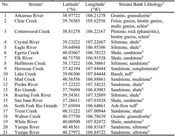
Table 1. Stream sites used by Jarrett (1984)
No. Stream1 Latitude1
(°N) Longitude 1
(°W) Stream Bank Lithology
2
1 Arkansas River 38.97722 106.21278 Granite, granodiorite3 2 Clear Creek 39.76583 105.62556 Felsic gneiss, biotite gneiss,
mafic gneiss, schist3 3 Cottonwood Creek 38.81278 106.22167 Plutonic rock (phaneritic),
biotite gneiss, schist3 4 Crystal River 39.23222 107.22667 Siltstone, shale4 5 Eagle River 39.64944 106.95306 Siltstone, shale4 6 Egeria Creek 40.03667 106.78222 Shale, sandstone4
7 Elk River 40.71750 106.91528 Shale, sandstone4
8 Halfmoon Creek 39.17222 106.38861 Siltstone, sandstone4 9 Hermosa Creek 37.42194 107.84444 Sandstone, conglomerate4 10 Lake Creek 39.06306 107.84444 Basalt, tuff3
11 Mad Creek 40.56556 106.88861 Sandstone, mudstone4 12 Piedra River 37.22222 107.34222 Sandstone, shale4 13 Rio Grande 37.76694 106.83083 Sandstone, shale4 14 Roaring Fork River 39.54361 107.32889 Siltstone, shale4 15 San Juan River 37.26611 107.01028 Shale, sandstone4 16 Sorth Fork Rio Grande 37.65694 106.64861 Ash-flow tuff3 17 Trout Creek 40.31222 107.00944 Sandstone, shale4 18 Walton Creek 40.57750 106.78639 Granite, granodiorite3 19 White River 40.00500 107.82472 Shale, sandstone4 20 Yampa River 40.48361 106.83167 Sandstone, siltstone4 21 Yampa River 40.27972 106.84722 Sandstone, siltstone4 1Site numbers, names and locations from Jarrett (1984).
2Stream bank lithology obtained by comparing locations with USGS (2005). 3Classified as crystalline.
4Classified as clastic sedimentary.
2. Materials and Methods
For the database used by Jarrett (1984), the stream bank lithology was determined by comparing the stream sites with the lithologies given in USGS (2005). If the site was mapped as alluvial material, then the lithology of the adjacent geologic unit (equivalent to the stream bank) was chosen. For all new measurements of the Manning roughness coefficient, the site locations were determined using the Garmin eTrex 10 GPS Receiver, and compared with geological maps for Haiti (Haiti Data 2015) and Utah (Constenius et al. 2011).
Stream discharge was measured by dividing streams wider than 10 feet into 20-30 sections of equal width and narrower streams into sections of equal width no smaller than six inches. Both depth and velocity were measured in the middle of each section. The velocity was measured with the USGS Pygmy Current Meter Model 6205 (Rickly Hydrological Company) over a 60-second period at a distance below the water surface equal to 60% of the depth. The slope of the water surface was measured by optical
surveying using the Topcon AT-B2 Auto Level. Eq. (1) was combined with the continuity equation
𝑄 = 𝑣𝐴 (3)
where Q is discharge and A is cross-sectional area, and inverted to solve for the Manning roughness coefficient
𝑛 =1.49𝐴𝑅(/*𝑆,/(
𝑄 (4)
Table 2a. Stream sites in Haiti: Site information
No. Stream Latitude1
(°N)
Longitude1 (°W)
Stream Bank Lithology2 H1 Tenèbre Rivière 19.38272 71.82659 Diorite, tonalite3 H2 Dlo Carice Rivière 19.38295 71.82793 Diorite, tonalite3 H3 Maricotte Rivière 19.38890 71.84020 Diorite, tonalite3 H4 Jean Denante Rivière 19.44689 71.75580 Diorite, tonalite3 H5 Grande Rivière du Nord 19.63907 72.16946 Andesite, rhyodacite3 H6 Biquini Rivière 19.63039 72.24890 Andesite, rhyodacite3
H7 Galois Rivière 19.65517 72.26888 Andesite, rhyodacite3
H8 Rivière Salé 19.69597 72.29568 Andesite, rhyodacite3
H9 Limbé Rivière 19.70647 72.39270 Andesite, rhyodacite3
H10 Namoreau Rivière 19.88595 72.82957 Limestone, marl4
H11 Grande Rivière 19.88653 72.83005 Limestone, marl4
1Coordinate system is WGS 84.
2Stream bank lithology obtained by comparing locations with Haiti Data (2015). 3Classified as crystalline.
4Classified as carbonate.
Table 2b. Stream sites in Haiti: Stream properties
No. Water Slope, S Hydraulic Radius, R (ft) Manning Roughness Coefficient, n
H1 0.0048 0.821 0.406 H2 0.0040 0.280 0.099 H3 0.0032 0.704 0.562 H4 0.0056 0.441 0.163 H5 0.0023 0.457 0.066 H6 0.0114 0.124 0.108 H7 0.0036 0.592 0.115 H8 0.0023 0.178 0.036 H9 0.0046 0.556 0.049 H10 0.0364 0.430 0.154 H11 0.0071 0.568 0.058
3. Results
The stream sites used by Jarrett (1984) were initially separated into 15 sites incising clastic sedimentary bedrock and six sites incising crystalline bedrock. The tendency of the crystalline stream sites to plot in the region of positive residuals of ln n and the
and ln R underpredict ln n for these sites (see Fig. 1a). This result is consistent with the tendency of crystalline rocks to erode into larger particles, compared with clastic
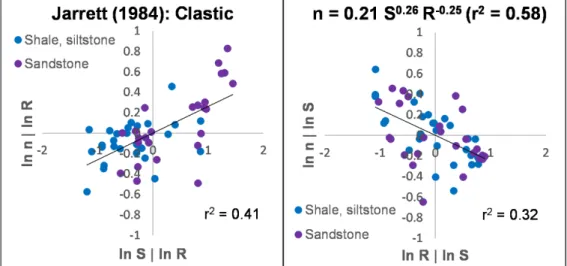
sedimentary rocks, and suggests that different multiple regression formulae should be used for the two generalized lithologies. However, removing the sites with crystalline stream banks only slightly improved the fit of the multiple regression formula (from r2 = 0.56 to r2 = 0.58, see Figs. 1a-b), probably because most of the measurements (54 out of 75) were on sites with clastic stream banks. When only the sites with clastic sedimentary stream banks were considered, there was some tendency for the sites with coarser-grained (primarily sandstone) banks to plot in the region of positive residuals of ln n and for the sites with finer-grained (primarily shale/siltstone) banks to plot in the region of negative residuals of ln n (see Fig. 1b), which is consistent with the greater flow resistance that should result from larger sediment. Separating the sites with sandstone and shale/siltstone banks resulted in an improved fit for sandstone sites alone (r2 = 0.63), but not for shale/siltstone sites alone (r2 = 0.53). Finally, considering only the stream sites with crystalline banks resulted in a poor regression fit (r2 = 0.10, see Fig. 1c), probably due to the very wide variety of crystalline rock types represented in the database (see Table 1).
Fig 1b. Based on the data set of Jarrett (1984), the ability of hydraulic radius R and water slope S to predict the Manning roughness coefficient n for high-gradient streams is slightly improved by considering only those stream sites that are incising clastic sedimentary rock. Separating the sites with sandstone and shale/siltstone banks resulted in an improved fit for sandstone sites alone (r2 = 0.63), but not for shale/siltstone banks alone (r2 = 0.53). On the left-hand plot, the residual of regressing ln n against ln R is shown as a function of the residual of regressing ln S against ln R. On the right-hand plot, the residual of regressing ln n against ln S is shown as a function of the residual of regressing ln R against ln S.
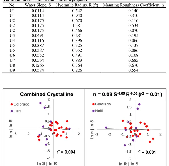
When the 21 measurements carried out by Jarrett (1984) at high-gradient stream sites incising crystalline bedrock were combined with the measurements at nine high-gradient sites incising crystalline bedrock in Haiti, the multiple regression fit was very poor (r2 = 0.01, see Fig. 2a), probably due to mixing stream sites from continental and tropical weathering environments. Restricting the stream sites to Haiti significantly improved the ability of slope and hydraulic radius to predict the Manning roughness coefficient (r2 = 0.46, see Fig. 2b). The regression formula tends to underpredict the Manning roughness
coefficient for streams incising diorite/tonalite and overpredict the Manning roughness coefficient for streams incising andesite/rhyodacite, which is consistent with the larger sediment derived from coarser-grained rocks (diorite/tonalite).
Fig 1c. Based on the data set of Jarrett (1984), the ability of hydraulic radius R and water slope S to predict the Manning roughness coefficient n for high-gradient streams is greatly reduced by considering only those stream sites that are incising crystalline rock. The poor fit is probably due to the wide range of crystalline rock types at the Colorado sites (see Table 1). On the left-hand plot, the residual of regressing ln n against ln
R is shown as a function of the residual of regressing ln S against ln R. On the right-hand plot, the residual of
regressing ln n against ln S is shown as a function of the residual of regressing ln R against ln S. Table 3a. Stream sites in Utah: Site information
No. Stream Latitude1
(°N) Longitude
1
(°W) Stream Bank Lithology2
U1 Right Fork Hobble Creek 40.16313 111.49931 Limestone
U2 Right Fork Hobble Creek 40.16721 111.49117 Limestone
U3 Tributary, South Fork Provo River 40.33374 111.52430 Limestone
U4 South Fork Provo River 40.34766 111.54687 Limestone
U5 Tributary, North Fork Provo River 40.37314 111.58029 Limestone
U6 North Fork Provo River 40.38349 111.57239 Limestone
U7 North Fork Provo River 40.37843 111.56836 Limestone
U8 Tributary, Hobble Creek 40.13144 111.52839 Limestone
U9 Tributary, Hobble Creek 40.13271 111.52518 Limestone
1Coordinate system is WGS 84.
2Bedrock lithology obtained by comparing locations with Constenius et al. (2011).
Combining 13 discharge measurements carried out at high-gradient stream sites
incising carbonate bedrock in Utah (see Table 3a) with two measurements at high-gradient sites incising carbonate bedrock in Haiti (see Table 2a) showed that 47% of the variation in the Manning roughness coefficient could be predicted by the variation in hydraulic radius and slope (see Fig. 3). The tendency of the stream sites in Haiti to plot in the region of negative residuals of ln n and below the best-fit regression line indicates that both ln S and ln R overpredict n for these sites. This result is consistent with the tendency of carbonate rocks to erode into smaller and more rounded particles in the tropical climate of Haiti.
Table 3b. Stream sites in Utah: Stream properties
No. Water Slope, S Hydraulic Radius, R (ft) Manning Roughness Coefficient, n
U1 0.0114 0.542 0.140 U1 0.0114 0.940 0.310 U2 0.0175 0.670 0.116 U2 0.0175 1.581 0.534 U2 0.0175 0.466 0.070 U3 0.0491 0.281 0.195 U4 0.0116 0.396 0.066 U5 0.0387 0.525 0.137 U5 0.0387 0.552 0.086 U6 0.0552 0.491 0.108 U7 0.0564 0.883 0.685 U8 0.1265 0.364 0.670 U9 0.0584 0.226 0.554
Fig 2a. Combining the 21 discharge measurements carried out by Jarrett (1984) at six high-gradient stream sites incising crystalline bedrock in Colorado with nine measurements at nine high-gradient sites incising crystalline bedrock in Haiti showed that only 1% of the variation in the Manning roughness coefficient n could be predicted by the variation in hydraulic radius R and water slope S. The poor fit is probably due to the wide range of crystalline rock types and the different weathering environments. On the left-hand plot, the residual of regressing ln n against ln R is shown as a function of the residual of regressing ln S against ln R. On the right-hand plot, the residual of regressing ln n against ln S is shown as a function of the residual of regressing ln R against ln S.
The 14 high-gradient canal sites in Utah included four types of canals (see Fig. 4, Table 4a). For the four canals lined with concrete with a trowel finish, all of the measured values of the Manning roughness coefficient (0.027-0.066) exceeded the typical maximum value of n = 0.015 (Chow, 1959, see Tables 4a-b). The higher values for high-gradient canals probably resulted from the tendency of rapid flows to strip away the trowel finish to expose the rough aggregate underneath. In the case of the Mt. Nebo Canal (see Table 4a), the very rough sides in the lower part of the canal wall could result from shallow,
left-hand side of Fig. 4). For the five earthen canals with cobble bottoms and banks, it was also found that all of the measured values of the Manning roughness coefficient (0.083-0.104) exceeded the typical maximum value of n = 0.050 (Chow, 1959, see Tables 4a-b). For these canals, the cobbles were not transported by flow, but were simply placed for
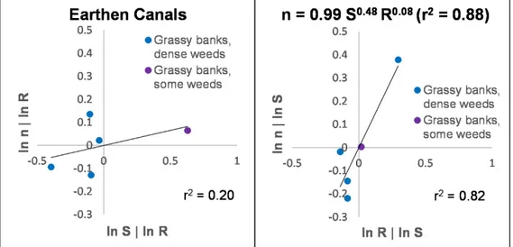
decoration and stabilization. For steep canals, it is likely that, in order to stabilize the canal banks, larger cobbles would be used than would be typical in much more common low-gradient canals, leading to a larger roughness coefficient. For the five earthen canals with grassy, weedy banks, the measured values of the Manning roughness coefficient (0.027-0.049) were not much different from the typical range (0.025-0.040). For these canals, hydraulic radius and slope were excellent predictors of the roughness coefficient (r2 = 0.88, see Fig. 5), with hydraulic radius being a much stronger predictor (see right-hand side of Fig. 5). The single canal with fewer weeds did not appear to be an outlier (see Fig. 5).
Fig. 2b. The ability of hydraulic radius R and water slope S to predict the Manning roughness coefficient n for high-gradient streams incising crystalline bedrock is greatly improved by considering only stream sites in Haiti and excluding stream sites in Colorado. On the left-hand plot, the residual of regressing ln n against ln
R is shown as a function of the residual of regressing ln S against ln R. On the right-hand plot, the residual of
regressing ln n against ln S is shown as a function of the residual of regressing ln R against ln S.
4. Discussion
The chief difference among the multiple regression formulae is that, in that, in the case of streams with clastic stream banks, the Manning roughness coefficient is a negative function of the hydraulic radius, while, in all other cases, the roughness coefficient is a positive function of the hydraulic radius (see Table 5a). In the case of clastic sediment, which tends to be more angular, turbulent resistance is mainly caused by the roughness of the sediment, the effect of which decreases as the water becomes deeper. However, in the case of crystalline or carbonate sediment, which tends to be more rounded, turbulent resistance is mainly caused by the increase in the Reynolds number, which is proportional to the depth. By combining the formulae for the roughness coefficient with Eq. (1), it can be seen that average velocity is an positive function of hydraulic radius for streams with clastic banks and earthen canals with grassy banks, but a negative function of hydraulic radius for streams with crystalline or carbonate banks (see Table 5b).
Fig 3. Combining 13 discharge measurements carried out at high-gradient stream sites incising carbonate bedrock in Utah with two measurements at high-gradient sites incising carbonate bedrock in Haiti showed that 47% of the variation in the Manning roughness coefficient n could be predicted by the variation in hydraulic radius R and water slope S. On the left-hand plot, the residual of regressing ln n against ln R is shown as a function of the residual of regressing ln S against ln R. On the right-hand plot, the residual of regressing ln n against ln S is shown as a function of the residual of regressing ln R against ln S.
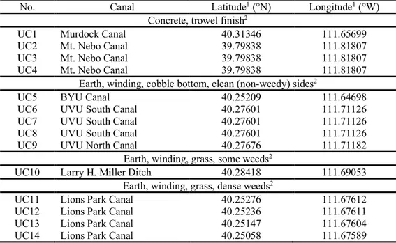
Table 4a. Canal sites in Utah: Site information
No. Canal Latitude1 (°N) Longitude1 (°W)
Concrete, trowel finish2
UC1 Murdock Canal 40.31346 111.65699
UC2 Mt. Nebo Canal 39.79838 111.81807
UC3 Mt. Nebo Canal 39.79838 111.81807
UC4 Mt. Nebo Canal 39.79838 111.81807
Earth, winding, cobble bottom, clean (non-weedy) sides2
UC5 BYU Canal 40.25209 111.64698
UC6 UVU South Canal 40.27601 111.71126
UC7 UVU South Canal 40.27601 111.71126
UC8 UVU South Canal 40.27601 111.71126
UC9 UVU North Canal 40.27676 111.71182
Earth, winding, grass, some weeds2
UC10 Larry H. Miller Ditch 40.28418 111.69053
Earth, winding, grass, dense weeds2
UC11 Lions Park Canal 40.25276 111.67612
UC12 Lions Park Canal 40.25236 111.67611
UC13 Lions Park Canal 40.25147 111.67604
UC14 Lions Park Canal 40.25058 111.67589
1Coordinate system is WGS 84.
Table 4b. Canal sites in Utah: Flow properties
No. Water Slope, S Hydraulic Radius, R (ft) Manning Roughness Coefficient, n Min n = 0.011, Normal n = 0.013, Max n = 0.0151
UC1 0.0019 0.086 0.027
UC2 0.3669 0.246 0.050
UC3 0.1755 0.288 0.046
UC4 0.0416 0.296 0.066
Min n = 0.030, Normal n = 0.040, Max n = 0.0501
UC5 0.0019 0.167 0.104
UC6 0.0240 0.029 0.095
UC7 0.0240 0.029 0.115
UC8 0.0240 0.029 0.095
UC9 0.0090 0.149 0.083
Min n = 0.025, Normal n = 0.030, Max n = 0.0331
UC10 0.0120 0.506 0.034
Min n = 0.030, Normal n = 0.035, Max n = 0.0401
UC11 0.0052 0.726 0.049
UC12 0.0060 0.463 0.033
UC13 0.0043 0.506 0.029
UC14 0.0059 0.490 0.027
1Typical minimum, normal and maximum values of Manning roughness coefficient for a given type of canal are
taken from Chow (1959). Note that the right-hand column is the measured Manning roughness coefficient at a particular canal site.
Fig. 4. Many canals in Utah were constructed along very steep slopes. In the left-hand photo, the Mt. Nebo Canal (Site UC2, see Table 4a) descends along a slope S = 0.3669. In the lower part of the canal wall, the concrete finish has been stripped away to expose the rough aggregate underneath. In the right-hand photo, the Lions Park Canal (Site UC11, see Table 4a) is an earthen canal with banks of grass and dense weeds,
The provisional formulae for the Manning roughness coefficient assume the most generalized categories that are reasonably possible based upon the results of this study (see Table 5a-b). For example, measurements in Colorado and Utah are assumed to be
representative of a continental climate, while measurements in Haiti are assumed to be representative of a tropical climate. Moreover, diorite/tonalite and andesite/rhyodacite are assumed to be representative of crystalline rock (see Tables 2a, 5a-b), while limestone and marl are assumed to be representative carbonate rocks (see Tables 2a, 3a, 5a-b). Clearly, more studies are needed that would either refine the categories or confirm the generalized categories. Up to this point, studies of flow resistance in mountain streams have neither documented stream bank lithology nor used lithology as an experimental control (e.g., Jarrett 1984; Reid and Hickin 2008; Asano et al. 2012; Zink and Jennings 2014).
Fig 5. Based on discharge measurements carried out at five high-gradient earthen canal sites in Utah, 88% of the variation in the Manning roughness coefficient n could be predicted by the variation in hydraulic radius R and water slope S. All earthen canal sites had grassy banks with some or dense weeds. On the left-hand plot, the residual of regressing ln n against ln R is shown as a function of the residual of regressing ln S against ln
R. On the right-hand plot, the residual of regressing ln n against ln S is shown as a function of the residual of
regressing ln R against ln S.
Table 5a. Provisional Formulae for Manning Roughness Coefficient in High-Gradient Canals and Natural Streams
Climate Substrate Formula1,2
Natural Streams
Continental Clastic Rock 𝑛 = 𝑒(2,.78 ± 0.(()𝑆(0.(1 ± 0.0<)𝑅(20.(7 ± 0.07) Tropical Crystalline Rock 𝑛 = 𝑒(*.,* ± *.*1)𝑆(0.=> ± 0.78)𝑅(0.>= ± 0.<7) Continental/Tropical Carbonate Rock 𝑛 = 𝑒(,.1, ± ,.0<)𝑆(0.=8 ± 0.(7)𝑅(0.8( ± 0.<,)
Canals
Continental Earth, Grassy Banks 𝑛 = 𝑒(20.0, ± 0.0,)𝑆(0.<8 ± 0.=*)𝑅(0.08 ± 0.0() 1n = Manning roughness coefficient, S = slope of water surface, R = hydraulic radius (ft)
2 Uncertainties are standard errors.
It is important to reinforce that the Manning roughness coefficient for mountain streams can often vastly exceed the commonly quoted range of n = 0.030-0.070 (Dingman
2009). The largest value found in this study was n = 0.685 (see Table 3b). Jarrett (1984) measured the roughness coefficient as high as n = 0.159, while Reid and Hickin (2008) measured a roughness coefficient of n = 7.95. Underestimating the Manning roughness coefficient can result in an overestimation of the resources available in mountain streams, such as the fluvial power available for generation of electricity. Moreover, underestimating the Manning roughness coefficient overestimates the ability of a mountain stream to accommodate an increase in stream discharge, thus underestimating the flooding potential of mountain streams under the impact of severe storms.
Table 5b. Manning Equations based upon Provisional Formulae for Manning Roughness Coefficient in High-Gradient Canals and Natural Streams
Climate Substrate Manning Equations1,2
Natural Streams
Continental Clastic Rock 𝑣 = 7.24𝑅0.>(𝑆0.(< Tropical Crystalline Rock 𝑣 = 0.065𝑅20.*0𝑆20.(> Continental/Tropical Carbonate Rock 𝑣 = 0.30𝑅20.,7𝑆20.(8
Canals
Continental Earth, Grassy Banks 𝑣 = 1.51𝑅0.7>𝑆0.0( 1The Manning Equations were obtained by combining Eq. (1) with Table 5a.
2 v = average velocity (ft/s), R = hydraulic radius (ft), S = slope of water surface
Acknowledgements. This research was completed as course projects for ENVT 3790 Hydrology I
and ENVT 4890 Surface Water Hydrology. We are grateful to Dr. Eddy Cadet for organizing the trip to Haiti and to UVU for funding from a Grant for Engaged Learning and an Undergraduate Research and Scholarly Activity Grant.
References
Arcement, G.J., and V.D. Schneider, 1989: Guide for selecting Manning’s roughness coefficients for natural channels and flood plains. U.S. Geological Survey Water Supply Paper 2339, 38 p.
Asano, Y., S. Hoshino, T. Uchida, and K. Akiyama, 2012: Measuring the flow and Manning’s roughness coefficient of mountain streams. Shin Sabo = Journal of the Japan Society of Erosion Control
Engineering, 65, 62-68.
Bathurst, D., 1985: Flow resistance estimation in mountain rivers. Journal of Hydraulic Engineering, 111, 625-643.
Chow, V.T., 1959: Open-channel Hydraulics. McGraw-Hill, 680 p.
Constenius, K. N., D. L. Clark, J. K. King, and J. B. Ehler, 2011: Interim geologic map of the Provo 30' x 60' quadrangle, Salt Lake, Utah, and Wasatch Counties. Utah Geological Survey OFR 586. Available online at https://ugspub.nr.utah.gov/publications/open_file_reports/ofr-586.pdf
Dingman, S. L., 2009: Fluvial Hydraulics. Oxford University Press, 559 p.
Dingman, S.L., and K.P. Sharma, 1997: Statistical development and validation of discharge equations for natural channels. Journal of Hydrology, 199, 13-35.
Haiti Data, 2015: Haiti Geology, BME [08.2005]. Available online at
http://haitidata.org/layers/cnigs.spatialdata:hti_geology_geology_polygon_082005
Jarrett, R.D., 1984: Hydraulics of high-gradient streams. Journal of Hydraulic Engineering, 110, 1519-1539. Marcus, W.A., K. Roberts, L. Harvey, and G. Tackman, 1992: An evaluation of methods for estimating
Manning’s n in small mountain streams. Mountain Research and Development, 12, 227-239.
Reid, D.E., and E.J. Hickin, 2008: Flow resistance in steep mountain streams. Earth Surface Processes and
Landforms, 33, 2211-2240.
USGS, 2005: Colorado Geologic Map Data. Available online at
https://mrdata.usgs.gov/geology/state/state.php?state=CO
Zink, J.M., and G.D. Jennings, 2014: Channel roughness in North Carolina mountain streams. Journal of the