Copyright © IEEE.
Citation for the published paper:
This material is posted here with permission of the IEEE. Such permission of the IEEE does
not in any way imply IEEE endorsement of any of BTH's products or services Internal or
personal use of this material is permitted. However, permission to reprint/republish this
material for advertising or promotional purposes or for creating new collective works for
resale or redistribution must be obtained from the IEEE by sending a blank email message to
pubs-permissions@ieee.org.
By choosing to view this document, you agree to all provisions of the copyright laws
protecting it.
2010
Using faults-slip-through metric as a predictor of fault-proneness
Wasif Afzal
Proceedings of the 17th Asia Pacific Software Engineering Conference (APSEC'10)
Using Faults-Slip-Through Metric As A Predictor of
Fault-Proneness
Wasif Afzal
Blekinge Institute of Technology PO Box 520, SE-372 25 Ronneby
Sweden
wasif.afzal@bth.se
ABSTRACT
Background: The majority of software faults are present in small number of modules, therefore accurate prediction of fault-prone modules helps improve software quality by focusing testing ef-forts on a subset of modules. Aims: This paper evaluates the use of the faults-slip-through (FST) metric as a potential predictor of fault-prone modules. Rather than predicting the fault-prone mod-ules for the complete test phase, the prediction is done at the spe-cific test levels of integration and system test. Method: We ap-plied eight classification techniques, to the task of identifying fault-prone modules, representing a variety of approaches, including a standard statistical technique for classification (logistic regression), tree-structured classifiers (C4.5 and random forests), a Bayesian technique (Naïve Bayes), machine-learning techniques (support vec-tor machines and back-propagation artificial neural networks) and search-based techniques (genetic programming and artificial im-mune recognition systems) on FST data collected from two large industrial projects from the telecommunication domain. Results: Using area under the receiver operating characteristic (ROC) curve and the location of (PF, PD) pairs in the ROC space, the faults-slip-through metric showed impressive results with the majority of the techniques for predicting fault-prone modules at both integra-tion and system test levels. There were, however, no statistically significant differences between the performance of different tech-niques based on AUC, even though certain techtech-niques were more consistent in the classification performance at the two test levels. Conclusions: We can conclude that the faults-slip-through metric is a potentially strong predictor of fault-proneness at integration and system test levels. The faults-slip-through measurements inter-act in ways that is conveniently accounted for by majority of the data mining techniques.
Categories and Subject Descriptors
D.2.8 [Software Engineering]: Metrics—Performance measures, Process metrics; D.2.9 [Software Engineering]: Management— Software quality assurance (SQA)
Permission to make digital or hard copies of all or part of this work for personal or classroom use is granted without fee provided that copies are not made or distributed for profit or commercial advantage and that copies bear this notice and the full citation on the first page. To copy otherwise, to republish, to post on servers or to redistribute to lists, requires prior specific permission and/or a fee.
Copyright 20XX ACM X-XXXXX-XX-X/XX/XX ...$10.00.
Keywords
Measurement, classification, reliability
1.
INTRODUCTION
The number of faults in a software module or in a particular release of a software represents quantitative measures of software quality. A fault prediction model uses historic software quality data in the form of metrics (including software fault data) to predict the number of software faults in a module or a release [28, 34]. Auto-matic prediction of fault-prone modules can be of immense value for a software testing team especially as we know that 20% of a software system is responsible for 80% of its errors, costs and re-work [3]. Some of the benefits of using software fault prediction include: (a) software quality can be improved by focussing on a subset of software modules. This in turn can reduce software fail-ures and hence the maintenance costs. (b) Refactoring candidates can be identified for reliability enhancement [12]. (c) Testing ac-tivities can be better planned.
While there is a plethora of studies on software quality classifi-cation (Section 2), none of them focus on identifying fault-prone modules at different test levels (such as unit, function, integration and system). Secondly, due to lack of quantification of quality at test levels, all the faults are assumed to be found at the right level which is not the case with many projects. This leads us to the con-cept of Faults-Slip-Through (FST) [15].
The Faults-Slip-Through (FST) concept is used for determining whether or not a fault slipped through the phase where it should have been found. The term phase refers to any phase in a typical software development life cycle. However the most interesting and industry-supported applications of FST measurement are during testing. This is because a defined testing strategy within any orga-nization implicitly classifies faults whereby certain types of faults might be targeted by certain strategies. FST is essentially a fault classification approach and focuses on when it is cost-effective to find each fault. Depending on the FST numbers for each test levels (e.g. unit, function, integration and system), improvement poten-tials can be determined by calculating the difference between the cost of faults in relation to what the fault cost would have been if none of them would have slipped through the level where they were supposed to be found. Thus, FST is a way to provide quantified de-cision support to reduce the effort spent on rework. This reduction in effort is due to finding faults earlier in a cost-effective way.
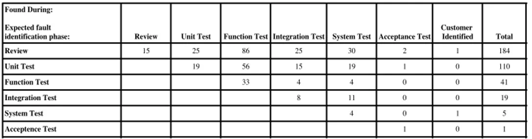
One way to visualize FST for different software testing phases is using an FST matrix (Figure 1).
The columns in Figure 1 represent the phases in which the faults were found (Found During), whereas the rows represent the phases where the faults should have been found (Expected fault identifi-cation phase). For example 56 of the faults that were found in
Report Name: Fault Slip Through Analysis Project: FST M570 Start Date: 2009-06-22 End Date: 2009-12-13 Customer Delivery: 2009-12-22
FST Measurement Tool
FST Matrix Found During:
Expected fault
identification phase: Review Unit Test Function Test Integration Test System Test Acceptance Test Customer Identified Total Output Slippage% Review 15 25 86 25 30 2 1 184 47 Unit Test 19 56 15 19 1 0 110 25 Function Test 33 4 4 0 0 41 2 Integration Test 8 11 0 0 19 3 System Test 4 0 1 5 0 Acceptence Test 1 0 1 0 Total 15 44 175 52 68 4 2 360 Input Slippage % 0 57 81 85 94 75 100 0
Review Unit Test Function Test Integration Test System Test Acceptance Test Customer Identified Total Incorrect data 76 1 8 25 1 0 0 0 111 24% Review Unit Test Function Test Integration Test System Test Acceptance Test Customer Identified
System Design Review, Module Design Review, Code Review HW Development, System Simulation, Module Test Function Test, Interoperability development test Integration of modules to functions, Integration Test System Test, IOT, Delivery Test
Type Approval
Customization, Customer Acceptance, Operator Identified, Customer Identified
Figure 1: An example FST matrix. function testing should have been found during unit testing.
In this paper we aim at predicting the fault-prone software mod-ules before integration and system test levels based on FST metric. The choice of these test levels is because they provide the last safety net before the software is released for customer use. In particular, we make use of number of faults slipping from unit and function test levels to predict the fault-prone modules at the integration and system test levels. We essentially seek an answer to the following research question:
RQ: How can we use FST to predict fault prone software modules before integration and system test and what is the resulting prediction performance?
The expectation is that answering this research question would provide valuable decision support for the project and test managers. This decision support relates to reduction in the number of faults slipping through to the end customer (lower maintenance and con-tended customers). We have used a number of classification tech-niques (logistic regression, C4.5, random forests, naïve Bayes, sup-port vector machines, artificial neural networks, genetic program-ming and artificial immune recognition systems) to the task of clas-sifying the quality of modules. We used FST and the associated affected modules’ data from two large industrial projects from the telecommunication domain. The results show that FST data is in-deed a strong predictor of quality of modules while majority of the classifiers show an appealing degree of classification performance. The main contributions of our paper are threefold: (a) It evaluates the use of FST metric as a potential predictor of fault-proneness. (b) It quantifies quality at specific test levels, i.e., integration and system. (c) It evaluates a range of classification techniques using trust-worthy evaluation criteria.
The remainder of the paper is organized as follows. Section 2 summarizes the related work. Section 3 describes the research con-text, including the variables and the data collection method. A brief on different classification techniques is given in Section 4. Sec-tion 5 gives an overview of how the performances of different tech-niques are evaluated. Results are given in Section 6 and are dis-cussed in Section 7. Validity evaluation and conclusions makeup Sections 8 and 9 respectively.
2.
RELATED WORK
There have been a number of techniques used for software qual-ity modeling (classifying fault-proneness or predicting number of software faults) based on different sets of metrics. The applica-ble techniques include statistical methods, machine learning meth-ods and mixed algorithms [14]. A number of metrics have been used as independent variables for software quality modeling and can broadly be classified into three categories [22]: (a) source code measures (structural measures), (b) measures capturing the amount
of change (delta measures) and, (c) measures collected from meta data in the repositories (process measures). Due to a large number of studies covering software quality modeling, the below references are more representative rather than exhaustive.
Gao and Khoshgoftaar [18] empirically evaluated eight statisti-cal count models for software quality prediction. They showed that with a very large number of zero response variables, the zero in-flated and hurdle-count models are more appropriate. The study by Yu et al. [47] used number of faults detected in earlier phases of the development process to predict the number of faults later in the process. They compared linear regression with a revised form of, an earlier proposed, Remus-Zilles model. They found a strong relationship between the number of faults during earlier phases of development and those found later, especially with their revised model. Khoshgoftaar et al. [27] showed that the typically used least squares linear regression and least absolute value linear regression do not predict software quality well when the data does not sat-isfy the normality assumption and thus two alternative parameter estimation procedures (relative least square and minimum relative error) were found more suitable in this case. In [37], the discrimi-nant analysis technique is used to classify the programs into either fault-prone and not fault-prone based upon the uncorrelated mea-sures of program complexity. Their technique was able to yield less Type II errors (mistakenly classifying a fault-prone module as fault-prone) on data sets from two commercial systems.
In [6], optimized set reduction classifications (that generates log-ical expressions representing patterns in the data) were found to be more accurate than multivariate logistic regression and clas-sification trees in modeling high-risk software components. The less optimistic results of using logistic regression are not in agree-ment with Khoshgoftaar’s study [24] which supports using logistic regression for software quality classification. Also the study by Denaro et al. [16] used logistic regression to successfully classify faults across homogeneous applications. Basili et al. [2] verified that most of the Chidamber and Kemerer’s object-oriented metrics are useful quality indicators for fault-prone classes. Ohlsson et al. [38] investigated the use of metrics for release n to identify the most fault-prone modules in release n + 1. Later, in [39], principal component analysis and discriminant analysis was used to rank the software modules in several groups according to fault-proneness.
Using the classification and regression trees (CART) algorithm, and by balancing the cost of misclassification, Khoshgoftaar et al. [25] showed that the classification-tree models based on several product, process and execution measurements were useful in qual-ity classification for successive software releases. Briand et al. [7] proposed multivariate adaptive regression splines (MARS) to clas-sify object-oriented (OO) classes as either prone or not fault-prone. MARS outclassed logistic regression with an added advan-tage that the functional form of MARS is not known a priori. In [36], the authors show that static code attributes like McCabe’s and
Halstead’s are valid attributes for fault prediction. It was further shown that naive Bayes outperformed the decision tree learning methods.
A number of studies have shown encouraging results using arti-ficial neural networks (ANNs) as the prediction technique [23, 30]. Cai et al. [10] observed that the prediction results of ANNs show a positive overall pattern in terms of probability distribution but were found to be poor at quantitatively estimating the number of software faults.
A study by Gray et al. [20] showed that neural network mod-els show more predictive accuracy as compared with regression based methods. The study also used a criteria-based evaluation on conceptual requirements and concluded that not all modeling techniques suit all types of problems. CART-LAD (least absolute deviation) performed the best in a study by Khoshgoftaar et al. [29] for fault prediction in a large telecommunications system in com-parison with CART-LS (least squares), S-plus, regression tree al-gorithm, multiple linear regression, artificial neural networks and case-based reasoning.
Gyimothy et al. [21] used OO metrics for predicting the number of faults in classes using logical and linear regression, decision tree and neural network methods. They found that the results from these methods were nearly similar. A recent study by Lessman et al. [34] also concluded that, with respect to classification, there were no significant differences among the top-17 of the classifiers used for comparison in the study.
Apart from ANNs some authors have proposed using fuzzy mod-els [42] and support vector machines [19] for software quality pre-dictions. In the later years, interest has shifted to evolutionary and nature-inspired computation approaches for software quality clas-sification; examples include genetic programming [26], genetic al-gorithm [1], artificial immune recognition systems [13] and particle swarm optimization [11].
While it is clear that previous studies have focussed on predicting the fault-proneness of software modules, none of them quantify the quality of modules at different test levels. Quantification of quality of modules at different test levels promises to provide opportuni-ties of more focussed improvements at each test level. The current study is unique from previous studies in two ways. Firstly the study aims to provide indications of fault-prone modules before starting integration and system test levels. Secondly the classification of fault-prone modules is done by making use of faults-slip-through (FST) data.
3.
RESEARCH CONTEXT
The data used in this study comes from two large projects at a telecommunication company that develops mobile platforms and wireless semiconductors. The projects are aimed at developing platforms introducing new radio access technologies written using the C programming language. The average number of persons in-volved in these projects is approximately 250. We have data from 106 modules from the two projects. Since a high percentage of modules were reused in the two projects, we evaluate the fault-proneness of 106 modules as if they are from a single project. We use a 10-fold cross-validation to evaluate the performance of dif-ferent techniques.
The management of these projects follow the company’s gen-eral project model called PROPS (PROfessional Project Steering). PROPS is based on the concepts of tollgates, milestones and check-points to manage and control project deliverables. Tollgates repre-sent long-term business decisions while milestones are predefined events at the operating work level. The monitoring of these mile-stones is an important element of the project management model.
Figure 2: Division of requirements into work packages and modules, thereby meeting tollgates, milestones and check-points.
The checkpoints are defined in the development process to define the work status in a process.
At the operative work level, the software development is struc-tured around work packages. These works packages are defined during the project planning phase. The work packages are defined to implement change requests or a subset of a use-case, thus the definition of work packages is driven by the functionality to be de-veloped. An essential feature of work packages is that it allows for simultaneous work on different modules of the project at the same time by multiple teams. Figure 2 gives an overview of how a given project is divided into work packages that affects multiple mod-ules. The division of an overall system into sub-systems in driven by design and architectural constraints.
The prediction models in this study make use of number of faults that should have been found at test levels prior to integration and system test. Since these faults were cost-effective to be found at test levels earlier than integration and system test, they are said to have slipped-through from the earlier test levels. These earlier test levels in our case are review, unit and function levels. The purpose of different test levels, as defined at our subject company, is given below:
• Review: To find faults in the feasibility of requirements, de-sign and architecture.
• Unit: To find faults in module internal functional behavior e.g. memory leaks.
• Function: To find faults in functional behavior involving mul-tiple modules.
• Integration: To find configuration, merge and portability faults. • System: To find faults in system functions, performance and
Some of these earlier test levels are composed of constituent test activities that jointly make up the higher-order test levels. Follow-ing is the division of test levels (i.e. review, unit, function, integra-tion and system) into constituent activities at our subject organiza-tion:
• Review: Module design review, code review. • Unit: Hardware development, Module test. • Function: Function test.
• Integration: Integration of modules to functions, integration test.
• System: System test, delivery test.
We collected the fault data for different modules that slipped from review, unit and function test levels to the integration and sys-tem test levels. Thus we can classify the modules as being either fault-prone or non-fault-prone at the integration and system test lev-els based on whether a single or no fault slipped through to these test levels from earlier levels.
This association of modules, with the levels where the faults were to be found in them, provides an intuitive and easy way to identify fault-prone software modules at different test levels. For instance, consider a fault in module A that slipped from unit level and was not captured until at integration level. Now the module A which is already fault-prone at the unit level, is more costly for quality improvement at the later integration level due to the higher cost of finding and fixing the faults at that level. But due to cer-tain reasons (e.g. ambiguous requirements) the fault is not detected at the right level and slipped. The integration test level now has to detect both the faults that are expected to be found in this level and also any other faults that slipped from earlier levels of review, unit and function test. At this stage, any indication of fault-prone modules would help plan better for integration testing. Also since integration test (and system test for that matter) represents one of the last test levels before the system is delivered to the end-users, it is critical that these last test levels have accurate knowledge of where to focus the testing effort.
Therefore we are interested in identifying those modules that were fault-prone in earlier test levels of review, unit and function but the faults from these modules slipped to integration and sys-tem test levels where they were eventually found. With a historical backlog of faults slipping through from review, unit and function test to integration and system test, along with the affected mod-ules, it is possible to build prediction models to predict fault-prone modules for an on-going project before the commencement of in-tegration and system test levels.
Our data set contains nine count metrics and the descriptions are given in Table 1. The data set contains two additional attributes that represent the dependent variables: FP-I (fault-prone at integration test level) and FP-S (fault-prone at system test level). Each one of these metrics is collected for every module separately; for example SF-CR in Table 1 represents the count of faults slipping from code review for each module. The data regarding the number of faults slipping to/from different test levels is readily available from an automated report generation tool at the subject company that used data from an internally developed system for fault logging.
4.
A BRIEF BACKGROUND ON THE
TECH-NIQUES
Table 1: Metric descriptions. Metric Definition
SF-CR No. of faults slipping from (SF) code review (CR)
SF-MDR No. of faults slipping from (SF) module design review (MDR)
SF-R No. of faults slipping from (SF) review (R) SF-HD No. of faults slipping from (SF) hardware
de-velopment (HD)
SF-MT No. of faults slipping from (SF) module test (MT)
SF-U No. of faults slipping from (SF) unit level (U) SF-F No. of faults slipping from (SF) function level
(F)
ST-I No. of faults slipping to (ST) integration level (I)
ST-S No. of faults slipping to (ST) system level (S) We compare a variety of techniques for the purpose of predicting fault-prone modules at integration and system test. The techniques include a standard statistical technique for classification (logistic regression), tree-structured classifiers (C4.5 and random forests), a Bayesian technique (Naïve Bayes), machine-learning techniques (support vector machines and back-propagation artificial neural net-works) and search-based techniques (genetic programming and ar-tificial immune recognition systems). Below is a brief description of these methods while the detailed descriptions can be found in relevant references.
4.1
Logistic regression (LR)
Logistic regression is used when the dependent variable is di-chotomous (e.g. either fault-prone or non-fault-prone). Logistic re-gression does not assume that the dependent variable or the error terms be normally distributed. The form of the logistic regression model is:
log“1−pp ”= β0+ β1X1+ β2X2+ . . . + βkXk
where p is the probability that the fault was found in the module that slipped to either integration or system test and X1, X2,. . ., Xk
are the independent variables. β0,β1, . . ., βk are the regression
coefficients estimated using maximum likelihood. A multinomial logistic regression model with a ridge estimator, implemented as part of WEKA, was used with default parameter values.
4.2
C4.5
C4.5 is the most well-known algorithm in the literature for build-ing decision trees [32]. C4.5 first creates a decision-tree based on the attribute values of the available training data such that the internal nodes denote the different attributes, the branches corre-spond to value of a certain attribute and the leaf nodes correcorre-spond to the classification of the dependent variable. The decision tree is made recursively by identifying the attribute(s) that discriminates the various instances most clearly, i.e., having the highest informa-tion gain. Once a decision tree is made, the predicinforma-tion for a new instance is done by checking the respective attributes and their val-ues. For our experiments, standard pruning factors as in WEKA were used i.e. with a confidence factor of 0.25.
4.3
Random forests (RF)
Random forests is a collection of tree-structured classifiers [5]. A new instance is classified on each tree in the forest. Results of these trees is used for majority voting and the forest selects the
clas-sification having the most votes over all the trees in the forest. Each classification tree is built using a bootstrap sample of the data. The results were generated using 10 trees (the default value in WEKA).
4.4
Naïve Bayes (NB)
The naïve Bayes classifier is based on the Bayesian theorem. It analyses each data attribute independently and being equally im-portant. The naïve Bayes classifier assigns an instance skwith
at-tribute values (A1= V1, A2= V2, . . . , Am= Vm) to class Ciwith
maximum prob(Ci|(V1, V2, . . . , Vm)) for all i. The results were
generated using default parameter values in WEKA.
4.5
Support vector machines (SVM)
SVM algorithm classifies data points by finding an optimal lin-ear separator which possess the largest margin between it and the one set of data on one side and other set of examples on the other. The largest separator is found by solving a quadratic programming optimization problem. Using WEKA, the regularization parameter (c) was set at 1; the kernel function used was Gaussian (RBF ) and the bandwidth (r) of the kernel function was set to 0.5.
4.6
Artificial neural networks (ANN)
The development of artificial neural networks is inspired by the interconnections of biological neurons [40]. These neurons, also called nodes or units, are connected by direct links. These links are associated with numeric weights which shows both the strength and sign of the connection [40]. Each neuron computes the weighted sum of its input, applies an activation (step or transfer) function to this sum and generates output, which is passed on to other neurons. A three layer feed forward neural network model has been used in this study. The final ANN structure consisted of one input layer, one hidden layer and one output layer. The hidden layer consisted of five nodes while the output layer had two nodes representing each of the binary outcome. The number of independent variables in the problem determined the number of input nodes. The sig-moid and linear transfer functions have been used for the hidden and output nodes respectively.
4.7
Genetic programming (GP)
GP, an evolutionary computation technique, is an extension of genetic algorithms [33]. The population structures (individuals) in GP are not fixed length character strings but programs that, when executed, are the candidate solutions to the problem. For the sym-bolic regression application of GP, programs are expressed as syn-tax trees, with the nodes indicating the instructions to execute and are called functions (e.g. min, ∗, +, /), while the tree leaves are called terminals which may consist of independent variables of the problem and random constants (e.g. x, y, 3). The worth of an in-dividual GP program in solving the problem is assessed using a fit-ness evaluation. The control parameters limit and control how the search is performed like setting the population size and probabili-ties of performing the genetic operations. The termination criterion specifies the ending condition for the GP run and typically includes a maximum number of generations [9]. GP iteratively transforms a population of computer programs into a new generation of pro-grams using various genetic operators. Typical operators include crossover, mutation and reproduction. The details of genetic oper-ators are omitted due to space constraints but can be found in [41]. The GP programs were evaluated according to the sum of absolute differences between the obtained and expected results in all fitness cases,Pn
i=1| ei− e
0
i|, where eiis the actual fault count data, e
0
i
is the estimated value of the fault count data and n is the size of the data set used to train the GP models. The control parameters that
Table 2: GP control parameters.
Control parameter Value
Population size 50
Termination condition 500 generations
Function set {+,−,∗,/,sin,cos,log,sqrt}
Tree initialization Ramped half-and-half method
Probabilities of crossover, mutation, reproduction 0.8, 0.1, 0.1
Selection method roulette-wheel
were chosen for the GP system are shown in Table 2.
4.8
Artificial immune recognition system
(AIRS)
The concepts of artificial immune systems have been used to pro-duce a supervised learning system called artificial immune recog-nition system (AIRS) [45].
Based on immune network theory, [43] developed a resource limited artificial immune system and introduced the metaphor of an artificial recognition ball (ARB), a collection of similar cells. B-cells are anti-body secreting B-cells that is a response of the immune system against the attack of a disease. For the resource-limited AIS, a predefined number of resources exists. The ARBs compete based on their stimulation level. Least stimulated cells are removed while an ARB having higher stimulation value could claim more resources. The AIRS is based on the similar idea of a resource-limited system but many of the network principles were abandoned in favor of a simple population-based model [45].
The AIRS algorithm consists of five steps [45]: 1) Initializa-tion, 2) Memory cell identification and ARB generaInitializa-tion, 3) Compe-tition for resources and development of a candidate memory cell, 4) Memory cell introductionand 5) Classification. The details of each of these steps can be found in [45] and are omitted due to space constraints.
The WEKA plug-in for AIRS [8] has been used with the follow-ing parameters: Affinity threshold = 0.2, clonal rate = 10, hyper-mutation rate = 2, knn = 3, hyper-mutation rate = 0.1, stimulation value = 0.9 and total resources = 150.
5.
PERFORMANCE EVALUATION
We use the area under the receiver operating curve (AUC) as the performance evaluation measure for different classifiers. Area under the curve (AUC) [4] acts as a single scalar measure of ex-pected performance and is an obvious choice for performance as-sessment when ROC curves for different classifiers intersect [34] or if the algorithm does not allow configuring different values of the threshold parameter. AUC, as with the ROC curve, is also a gen-eral measure of predictive performance since it separates predictive performance from class and cost distributions [34]. The AUC mea-sures the probability that a randomly chosen fault-prone module has a higher output value than a randomly chosen non fault-prone module [17]. The value of AUC is always between 0 and 1; with a higher AUC is preferable indicating that the classifier is on average more effective in identifying fault prone modules.
We also plotted the (PF, PD) pairs belonging to various classi-fication algorithms to facilitate visualization [35] (PF denotes the probability of false alarm, i.e., proportion of non-fault prone mod-ules that are erroneously classified and PD denotes the probability of detection of fault-prone modules).
6.
EXPERIMENTAL RESULTS
The (PF, PD) pairs for different techniques for detecting fault-prone software modules at integration test level are given in
Ta-Table 3: (PF, PD) pairs for fault prediction at integration test level. Techniques PF PD GP 0 0.98 LR 0.04 0.94 C4.5 0 0.98 RF 0 0.96 NB 0.49 0.94 SVM 0 0 ANN 0.90 0.98 AIRS 0.24 0.70
Figure 3: (PF, PD) pairs for different techniques for fault pre-diction at integration test level.
ble 3. The corresponding location of these pairs in the ROC space is shown in Figure 3.
It is encouraging to note that six out of eight classifiers (GP, LR, C4.5, RF, NB, AIRS) are placed in the upper left region of the ROC space which is the region of interest for the software engineers, marked by high probability of detection (PD) and low probability of false alarm (PF). In fact, four out of these six classifiers (GP, LR, C4.5, RF) are approximately equal to the perfect (PF, PD) pair of (0, 1). Out of these four classifiers, GP and C4.5 are slightly better placed than LR and RF but the differences are minimal. SVM and ANN show less impressive performances and thus offer little decision-support to the software engineers.
One way to quantify the distances of individual (PF, PD) pairs from the perfect classification (0, 1) is to use a distance metric, ED [35]:
ED =pΘ ∗ (1 − P D)2+ (1 − Θ) ∗ P F2
where Θ (ranging from 0 to 1) represents the weights assigned to PD and PF. If we assume that lower PD is more costly than a higher PF, one can assign more weight to (1 − P D). Table 4 calculates the distance metric, ED, for the four visibly better classifiers for an arbitrary range of Θ values. The smaller the distance, i.e., the closer the point is to the perfect classification, the better the perfor-mance of the classifier [35]. GP and C4.5 show smaller distances in comparison with other two classifiers; a trend that is also confirmed from visualizing their (PF, PD) pairs in Figure 3.
Table 5 shows the AUC measures for different techniques for predicting fault-prone modules at integration test level. GP, LR, C4.5 and RF show higher AUC values than others for fault
predic-Table 4: Distance metric, ED, values for the four better tech-niques for fault prediction at integration test level.
Θ ED_GP ED_LR ED_C4.5 ED_RF
1 0.02 0.06 0.02 0.04
0.9 0.019 0.058 0.019 0.038 0.8 0.018 0.056 0.018 0.036 0.7 0.017 0.055 0.017 0.033 0.6 0.015 0.053 0.015 0.031 Table 5: AUC measures for different techniques at integration test level.
GP LR C4.5 RF NB SVM ANN AIRS 0.99 0.95 0.99 0.98 0.73 0.50 0.54 0.73 tion at the integration test level.
The (PF, PD) pairs for different techniques for detecting fault-prone modules at system test level are given in Table 6. The cor-responding location of these pairs in the ROC space is shown in Figure 4. As was the case with integration test level, most of the techniques (with the exception of SVM) have their (PF, PD) pairs in the preferred upper left region of the ROC space. Four of the techniques (GP, LR, C4.5, RF) give the perfect classification per-formance having the (PF, PD) pairs equal to (0, 1), while NB is close to having a perfect performance. SVM is not able to pro-vide useful results, with high probability of false alarms. ANN and AIRS are able to provide moderate (PF, PD) pairs. The perfect classification performance of four techniques (GP, LR, C4.5, RF) renders zero distance metric, ED, which is the best-case scenario. Table 7 shows the AUC measures for different techniques for pre-dicting fault-prone modules at system test level. As expected, the four techniques (GP, LR, C4.5, RF) have perfect AUC values with NB not far behind.
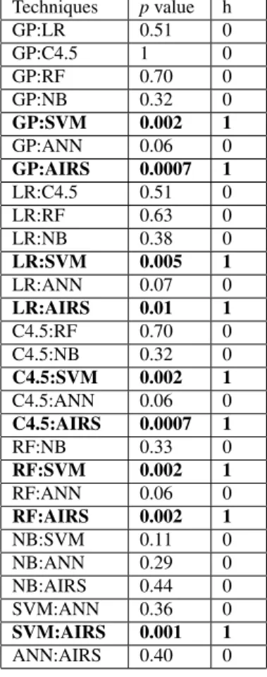
Now that we have the AUC values for different techniques for predicting fault-prone modules at integration and system test lev-els, we can use a two-sample t-test to verify if the differences in AUC values among different pairs of techniques are significant or not. The results of applying the two sample t-test appear in Table 8 where h = 1 indicates a rejection of the null hypothesis at 5% sig-nificance level of the two samples having equal means, while h = 0 indicates a failure to reject the null hypothesis at 5% significance level.
The results show that apart from nine combinations, highlighted in bold in Table 8, there are no significant differences between the AUC values of all other combination of classifiers.
7.
DISCUSSION
In this paper, we evaluated the use of several techniques for
pre-Table 6: (PF, PD) pairs for fault prediction at system test level. Techniques PF PD GP 0 1 LR 0 1 C4.5 0 1 RF 0 1 NB 0.08 1 SVM 0.90 0.98 ANN 0.24 0.70 AIRS 0.34 0.82
Figure 4: (PF, PD) pairs for different techniques for fault pre-diction at system test level.
Table 7: AUC measures for different techniques at system test level.
GP LR C4.5 RF NB SVM ANN AIRS 1 1 1 1 0.96 0.54 0.73 0.74
Table 8: Two-sample t-test results for differences in AUC mea-sures for different techniques.
Techniques pvalue h GP:LR 0.51 0 GP:C4.5 1 0 GP:RF 0.70 0 GP:NB 0.32 0 GP:SVM 0.002 1 GP:ANN 0.06 0 GP:AIRS 0.0007 1 LR:C4.5 0.51 0 LR:RF 0.63 0 LR:NB 0.38 0 LR:SVM 0.005 1 LR:ANN 0.07 0 LR:AIRS 0.01 1 C4.5:RF 0.70 0 C4.5:NB 0.32 0 C4.5:SVM 0.002 1 C4.5:ANN 0.06 0 C4.5:AIRS 0.0007 1 RF:NB 0.33 0 RF:SVM 0.002 1 RF:ANN 0.06 0 RF:AIRS 0.002 1 NB:SVM 0.11 0 NB:ANN 0.29 0 NB:AIRS 0.44 0 SVM:ANN 0.36 0 SVM:AIRS 0.001 1 ANN:AIRS 0.40 0
dicting fault-prone modules at integration and system test levels us-ing faults-slip-through data from two industrial projects. The most interesting result of this paper demonstrates the use of faults-slip-through metric as a potentially strong predictor of fault-proneness. While previous studies have focussed on structural measures, change measures and process measures (Section 2) as predictors of fault proneness, this study shows that the use of number of faults slip-ping through to/from various test levels are able to provide remark-able results for finding fault-prone modules at integration and sys-tem test levels. At integration test level, six out of eight techniques; while at the system test level, seven out of eight techniques resulted in impressive AUC values (0.7 or more – with their (PF, PD) pairs in the preferred region of the ROC space). This shows that the faults-slip-through measures have sufficient discriminative power to classify modules as either fault-prone and non-fault-prone at in-tegration and system test levels.
Previous studies on fault-proneness classified modules irrespec-tive of the different test levels. While such studies are useful, we might run into a risk of investing more effort in improving the qual-ity of a module than is cost-effective at a certain test level. The quantification of quality of modules at different test levels, cou-pled with the use of FST measures, entail an additional benefit that modules can be selected for quality enhancement keeping in view the cost-effectiveness. Thus the fundamental hypothesis underly-ing the work in this study is that an efficient test process verifies each product aspect at a test level where it is easiest to test and the faults are cheapest to fix; therefore the identification of fault-prone modules at specific test levels is a step in that direction. We were assisted in this endeavor to an extent by the segregation of different test levels at our subject organization.
The statistical comparison of the AUC values for different tech-niques at the two test levels present an interesting outcome, i.e., with few exceptions, most of the techniques did not differ signifi-cantly. This shows that the FST measures interact in ways that is conveniently accounted for by the different data mining techniques. However we need additional ways to visualize the performance of different techniques and the plotting of (PF, PD) pairs in the ROC space is one way of achieving it. As clear from the two plots in Figures 3 and 4, the location of (PF, PD) pairs in the ROC space can quickly show the trade-off in PF and PD values of competing techniques whereby one or more techniques might be preferred. This additional way to visualize performance is important from the viewpoint of practical use. A software manager who intends to ap-ply these techniques would be mainly interested in correct detection of fault-prone modules, i.e., PD [44]. This is because the cost of delivering fault-prone modules to the end-customers is much more than the cost of testing one module too many. This unequal costs of misclassification is the reason why software managers would pre-fer a trade-off between PF and PD. Using a distance metric like ED and visualizing the (PF, PD) pairs in the ROC space provides that flexibility to the software manager.
One trend that is observable from the results is that tree-structured classifiers (C4.5, RF), a search-based technique (GP) and a rather simple LR consistently perform remarkably well at both integra-tion and system test levels. For C4.5, RF and GP one addiintegra-tional advantage is the comprehensibility of the resulting models which can lead to an insight of the significant predictor variables and im-portant rules.
While working on-site at the subject organization for this re-search, we realized several organizational factors that influence the success of such a decision-support. Managerial support and an established organizational culture of quantitative decision-making helped easy access to data repositories and relevant documentation.
Moreover, collection of faults-slip-through data and association of that data to modules was made possible using an automated tool support that greatly reduced the time for data collection and en-sured data integrity.
8.
VALIDITY EVALUATION
There can be different threats to the validity of the empirical re-sults [46]. Conclusion validity refers to the statistically significant relationship between the treatment (independent variable) and the outcome (dependent variable). We tested for any significant differ-ences between the AUC values of different techniques using a two-sample t-test at 5% significance level, which is a commonly used significance level for hypothesis testing. The choice of selecting a parametric test was based on its greater power to identify differ-ences and robustness to smaller departures from the normality as-sumption. Internal validity refers to a causal relationship between treatment and outcome. Out of the many metrics we could collect, we only selected those based on the FST metric since our goal was to evaluate the use of such metrics for quality prediction. We used a 10-fold cross-validation as a resampling method which has been found to give low bias and low variance [31]. A potential threat to internal validity is that the faults-slip-through data did not consider the severity level of faults, rather treated all faults equally. Con-struct validityis concerned with the relationship between the the-ory and application. The use of AUC as the performance measure is motivated by the fact that it is a general measure of predictive performance, while the plot of (PF, PD) pairs provides an intuitive visualization tool. External validity is concerned with generaliza-tion of results outside the scope of the study. The data used in the study comes from two industrial projects from the telecommuni-cation domain and thus represents real-life use. However, more replications of this study would help generalize the results beyond the specific environment.
9.
CONCLUSION AND FUTURE WORK
This paper evaluated the used of faults-slip-through data as po-tential predictors of fault-proneness at integration and system test levels for data gathered from two industrial projects. A variety of classification algorithms were applied, including a standard statisti-cal technique for classification (logistic regression), tree-structured classifiers (C4.5 and random forests), a Bayesian technique (Naïve Bayes), machine-learning techniques (support vector machines and back-propagation artificial neural networks) and search-based tech-niques (genetic programming and artificial immune recognition sys-tems). The performance of these classifiers was assessed using AUC and location of (PF, PD) pairs in the ROC space. The re-sults of this study concluded that faults-slip-through data turns out to be a remarkable predictor of fault-proneness at integration and system test levels, with many of the techniques showing impressive AUC values and were located in the favorable region of the ROC space in terms of the (PF, PD) pairs. As for the different classifiers, although C4.5, RF, LR and GP performed more consistently across both integration and system test levels, the different classifiers did not differ significantly based on AUC. However, the visualization of (PF, PD) pairs in the ROC space provides another opportunity for the test team to assess a classifier performance with respect to the perfect (PF, PD) pair of (0, 1). A distance metric can then be calculated, with different weights assigned to represent the misclas-sification costs of PF and PD, to select a classifier most suited for the project.
Based on this paper, some interesting future work can be under-taken. Firstly, it would be interesting to compare the FST metric
with other commonly used predictors of fault proneness to quantify any differences. Secondly, the performance of FST as an effective predictor of fault-proneness need to be assessed for a segregation of faults based on severity levels. Lastly, one can think of a proba-bilistic model on how likely different fault counts or slips in earlier phases are for predicting fault-proneness in later phases.
10.
REFERENCES
[1] D. Azar, D. Precup, S. Bouktif, B. Kégl, and H. Sahraoui. Combining and adapting software quality predictive models by genetic algorithms. In Proceedings of the 17th IEEE international conference on Automated software engineering (ASE’02), Washington, DC, USA, 2002. IEEE Computer Society.
[2] V. R. Basili, L. C. Briand, and W. L. Melo. A validation of object-oriented design metrics as quality indicators. IEEE Transactions on Software Engineering, 22(10):751–761, 1996.
[3] B. Boehm. Industrial software metrics top 10 list. IEEE Software, 4(9):84–85, 1987.
[4] A. P. Bradley. The use of the area under the ROC curve in the evaluation of machine learning algorithms. Pattern
Recognition, 30:1145–1159, 1997.
[5] L. Breiman. Random forests. Machine Learning, 45(1):5–32, 2001.
[6] L. C. Briand, V. R. Basili, and C. J. Hetmanski. Developing interpretable models with optimized set reduction for identifying high-risk software components. IEEE
Transactions on Software Engineering, 19(11):1028–1044, 1993.
[7] L. C. Briand, W. L. Melo, and J. Wust. Assessing the applicability of fault-proneness models across
object-oriented software projects. IEEE Transactions on Software Engineering, 28(7):706–720, 2002.
[8] J. Brownlee. WEKA plug-in for AIRS. http://wekaclassalgos.sourceforge.net/, 2010.
[9] E. K. Burke and G. Kendall, editors. Search methodologies – Introductory tutorials in optimization and decision support techniques. Springer Science and Business Media, Inc., 2005.
[10] K. Y. Cai, L. Cai, W. D. Wang, Z. Y. Yu, and D. Zhang. On the neural network approach in software reliability modeling. Journal of Systems and Software, 58(1):47–62, 2001. [11] A. B. d. Carvalho, A. Pozo, and S. R. Vergilio. A symbolic
fault-prediction model based on multiobjective particle swarm optimization. Journal of Systems and Software, 83(5):868 – 882, 2010.
[12] C. Catal and B. Diri. Investigating the effect of dataset size, metrics sets, and feature selection techniques on software fault prediction problem. Information Sciences, 179(8):1040 – 1058, 2009.
[13] C. Catal, B. Diri, and B. Ozumut. An artificial immune system approach for fault prediction in object-oriented software. International Conference on Dependability of Computer Systems, 2007.
[14] V. U. B. Challagulla, F. B. Bastani, I. Yen, and R. A. Paul. Empirical assessment of machine learning based software defect prediction techniques. In Proceedings of the 10th IEEE international workshop on object-oriented real-time dependable systems (WORDS’05), Washington, DC, USA, 2005. IEEE Computer Society.
[15] L.-O. Damm, L. Lundberg, and C. Wohlin.
Faults-slip-through – a concept for measuring the efficiency of the test process. Software Process: Improvement and Practice, 11(1):47 – 59, 2006.
[16] G. Denaro and M. Pezze. An empirical evaluation of fault-proneness models. In Proceedings of the 24th International Conference on Software Engineering (ICSE’02), 2002.
[17] T. Fawcett. An introduction to ROC analysis. Pattern Recognition Letters, 27(8):861–874, 2006.
[18] K. Gao and T. Khoshgoftaar. A comprehensive empirical study of count models for software fault prediction. IEEE Transactions on Reliability, 56(2), 2007.
[19] I. Gondra. Applying machine learning to software
fault-proneness prediction. Journal of Systems and Software, 81(2):186–195, 2008.
[20] A. Gray and S. MacDonell. A comparison of techniques for developing predictive models of software metrics.
Information and Software Technology, 39(6), 1997. [21] T. Gyimothy, R. Ferenc, and I. Siket. Empirical validation of
object-oriented metrics on open source software for fault prediction. IEEE Transactions on Software Engineering, 31(10):897–910, 2005.
[22] E. B. Johannessen. Data mining techniques, candidate measures and evaluation methods for building practically useful fault-proneness prediction models. Master’s thesis, University of Oslo, Department of Informatics, Oslo, Norway.
[23] T. Khoshgoftaar, E. Allen, J. Hudepohl, and S. Aud. Application of neural networks to software quality modeling of a very large telecommunications system. IEEE
Transactions on Neural Networks, 8(4), 1997.
[24] T. M. Khoshgoftaar and E. B. Allen. Logistic regression modeling of software quality. International Journal of Reliability, Quality and Safety Engineering, 6(4):303–317, 1999.
[25] T. M. Khoshgoftaar, E. B. Allen, W. D. Jones, and J. I. Hudepohl. Classification tree models of software quality over multiple releases. In Proceedings of the 10th International Symposium on Software Reliability Engineering (ISSRE’99), Washington, USA, 1999. IEEE Computer Society.
[26] T. M. Khoshgoftaar and Y. Liu. A multi-objective software quality classification model using genetic programming. IEEE Transactions on Reliability, 56(2):237–245, 2007. [27] T. M. Khoshgoftaar, J. C. Munson, B. B. Bhattacharya, and
G. D. Richardson. Predictive modeling techniques of software quality from software measures. IEEE Transactions on Software Engineering, 18(11):979–987, 1992.
[28] T. M. Khoshgoftaar and N. Seliya. Tree-based software quality estimation models for fault prediction. In
Proceedings of the 8th International Symposium on Software Metrics (METRICS’02), Washington, DC, USA, 2002. IEEE Computer Society.
[29] T. M. Khoshgoftaar and N. Seliya. Fault prediction modeling for software quality estimation: comparing commonly used techniques. Empirical Software Engineering, 8(3):255–283, 2004.
[30] N. R. Kiran and V. Ravi. Software reliability prediction by soft computing techniques. Journal of Systems and Software, 81(4), 2008.
[31] R. Kohavi. A study of cross-validation and bootstrap for
accuracy estimation and model selection. In Proceedings of the 14th international joint conference on Artificial intelligence (IJCAI’95), San Francisco, CA, USA, 1995. Morgan Kaufmann Publishers Inc.
[32] S. B. Kotsiantis, I. D. Zaharakis, and P. E. Pintelas. Machine learning: A review of classification and combining
techniques. Artificial Intelligence Review, 26(3):159 – 190, 2007.
[33] J. Koza. GP: On the programming of computers by means of natural selection. MIT Press, Cambridge, MA, USA, 1992. [34] S. Lessmann, B. Baesens, C. Mues, and S. Pietsch.
Benchmarking classification models for software defect prediction: A proposed framework and novel findings. IEEE Transactions on Software Engineering, 34(4):485–496, 2008. [35] Y. Ma and B. Cukic. Adequate and precise evaluation of
quality models in software engineering studies. In Proceedings of the Third International Workshop on Predictor Models in Software Engineering (PROMISE’07), Washington, DC, USA, 2007. IEEE Computer Society. [36] T. Menzies, J. Greenwald, and A. Frank. Data mining static
code attributes to learn defect predictors. IEEE Transactions on Software Engineering, 33(1):2–13, 2007.
[37] J. C. Munson and T. M. Khoshgoftaar. The detection of fault-prone programs. IEEE Transactions on Software Engineering, 18(5):423–433, 1992.
[38] N. Ohlsson, A. C. Eriksson, and M. Helander. Early risk-management by identification of fault-prone modules. Empirical Software Engineering, 2(2):166–173, 1997. [39] N. Ohlsson, M. Zhao, and M. Helander. Application of
multivariate analysis for software fault prediction. Software Quality Journal, 7(1):51–66, 1998.
[40] S. Russell and P. Norvig. Artificial intelligence—A modern approach. Prentice Hall Series in Artificial Intelligence, USA, 2003.
[41] S. Silva. GPLAB—A genetic programming toolbox for MATLAB. http://gplab.sourceforge.net.
[42] S. S. So, S. D. Cha, and Y. R. Kwon. Empirical evaluation of a fuzzy logic-based software quality prediction model. Fuzzy Sets and Systems, 127(2):199–208, 2002.
[43] J. Timmis, M. Neal, and J. Hunt. An artificial immune system for data analysis. Biosystems, 55(1-3), 2000. [44] O. Vandecruys, D. Martens, B. Baesens, C. Mues, M. D.
Backer, and R. Haesen. Mining software repositories for comprehensible software fault prediction models. Journal of Systems and Software, 81(5):823–839, 2008.
[45] A. Watkins, J. Timmis, and L. Boggess. Artificial immune recognition system (AIRS): An immune-inspired supervised learning algorithm. GPEM, 5(3), 2004.
[46] C. Wohlin, P. Runeson, M. Höst, M. Ohlsson, B. Regnell, and A. Wesslén. Experimentation in software engineering: An introduction. Kluwer Academic Publishers, USA, 2000. [47] T. J. Yu, V. Y. Shen, and H. E. Dunsmore. An analysis of
several software defect models. IEEE Transactions on Software Engineering, 14(9):1261–1270, 1988.