Modeling Insurance Claim Sizes using the Mixture of Gamma & Reciprocal Gamma Distributions

Institutionen för Matematik och Fysik

Code: MdH-IMa-2005:018

MASTER THESIS IN MATHEMATICS /APPLIED MATHEMATICS

Modelling Insurance Claim Sizes using the Mixture of Gamma &

Reciprocal Gamma Distributions

by

Ying Ni

Magisterarbete i matematik / tillämpad matematik

DEPARTMENT OF MATHEMATICS AND PHYSICS

MÄLARDALEN UNIVERSITY

DEPARTEMENT OF MATHEMATICS AND PHYSICS

___________________________________________________________________________ Master thesis in mathematics / applied mathematics

Date:

2005-12-20

Project name:

Modelling Insurance Claim Sizes using the Mixture of Gamma & Reciprocal Gamma Distributions

Author:

Ying Ni

Supervisors:

Dmitrii Silvestrov, Anatoliy Malyarenko

Examiner:

Dmitrii Silvestrov

Comprising:

20 points

Abstract

A gamma-reciprocal gamma mixture distribution is used to model the claim size distribution. It is specially designed to handle both ordinary and extremely large claims. The gamma distribution has a lighter tail. This is meant to be a model for the frequent, small & moderate claims while the reciprocal gamma distribution covers the large, but infrequent claims.

We begin with introducing the gamma distribution and motivating its role in small & moderate claim size modelling, followed with a discussion on the reciprocal gamma distribution and its application in large claims size modelling; finally we demonstrate the mixture of gamma & reciprocal gamma as the generally applicable statistical model.

Two parameter estimation techniques, namely the method of moments and maximum likelihood estimation are provided to fit the single gamma, single reciprocal gamma, and the general mixture models. We shall explain in details the solution concepts of the involved moment estimation and likelihood equations. We shall even make an effort to evaluate the proposed moment estimation algorithm.

Two Java applications, namely the Java Mixture Model Simulation Program and the Java Mixture Model Estimation Program are developed to facilitate the analysis. While the former simulates samples that follow the mixture distribution given known parameters, the latter provides the parameter estimation for simplified cases given samples.

Keywords: Gamma distribution; Reciprocal gamma distribution; Mixture of gamma and reciprocal gamma; Claim size distribution; Large claim size distribution; Method of moments; Maximum likelihood estimation; Estimating the parameters of gamma; Estimating the parameters of reciprocal gamma

Notation & Abbreviations

Notation Pr (…) the probability of … ) (α Γ gamma function Γ =

∫

∞ − − 0 1 _. ) (_α xα e x dx ) (α ψ digamma function ( ) ln (a) d d _Γ = α α ψ ) ( ' α ψ trigamma function ) ; (α x

γ “lower” incomplete gamma function _x =

∫

x_t −_e−t_dt

0 1 ) ; (α α γ ) ; (α x

Γ “upper” incomplete gamma function Γ =

∫

∞ − −

x t_dt e t x₎ 1 ; (α α L likelihood function L

ln log likelihood function

2

α

χ chi-square distribution with a degrees of freedom Abbreviations

cdf cumulative distribution function mgf moment-generating function

MLE maximum likelihood estimation,

maximum likelihood estimator, or maximum likelihood estimate R-gamma reciprocal gamma (distribution)

Table of Contents

1. Introduction ………...…….………..……….. 1

2. The Gamma Distribution ……….……….. 2

2.1. Definition, Moments & Properties ………... 2

2.2. Applications in Claim Size Modelling ………. 5

2.3. Estimation of Parameters ……….. 6

2.3.1. Method of Moments Estimation …………..………..….. 7

2.3.2. Maximum Likelihood Estimation …….………. . 8

3. The Reciprocal Gamma Distribution ………... 12

3.1. Definition, Moments & Properties ……….. 12

3.2. Applications in Claim Size Modelling ……… 15

3.3. Estimation of Parameters ………. 15

3.3.1. Method of Moments Estimation ………..…15

3.3.2. Maximum Likelihood Estimation ………16

4. The Mixture of Gamma & Reciprocal Gamma ………... 17

4.1. The Mixture of Gamma & Reciprocal Gamma ………...….17

4.2. Estimation of Parameters ………...……….…18

4.2.1. Method of Moments Estimation ………. 18

4.2.2. Maximum Likelihood Estimation ……….. 24

5. Simulation Studies ………... 27 5.1. Simulation ………... 27 5.2. Estimation ………...………... 29 6. Conclusion ………... 39 7. References ………... 40 8. Appendixes .………..…... 41

Appendix A: Java Mixture Model Simulation Program-Users’ Guide …... 42

Appendix B: Java Mixture Model Estimation Program- Users’ Guide……...………. 46

Appendix C: Java Source Code: MixtureModelSimulation.java ...………….…….… 49

Appendix D: Java Source Code: MixtureModelEstimation.java ………….……….... 62

1. Introduction

It is not unusual that, in addition to a large number of “ordinary” policies, an insurance portfolio also contains a small number of policies under which much larger claim sizes are likely. Those large claims usually represent the greatest part of the indemnities paid by the insurer. It is therefore essential for actuary to have a good model, which takes consideration into those extreme large claims.

In this paper, we introduce a new and generally applicable statistical model for individual insurance claim sizes, the mixture of gamma and reciprocal gamma model, which is specially designed to handle both ordinary and extremely large claims. This model uses gamma distribution as the first component, placing probability p and reciprocal gamma distribution as the second, placing probability 1-p. The gamma distribution has a lighter tail. This is meant to be a model for the frequent, small claims while the reciprocal gamma distribution covers the large, but infrequent claims.

If we set p = 1, the general model reduces to the single gamma which is by itself important as a model for ordinary claim sizes, that is, data without heavy tails; At p = 0, it reduces to the single reciprocal gamma model, and because of the heavy tail of this distribution it can model the extremely large claims.

We shall discuss the statistical properties of the two component distributions, gamma and reciprocal gamma distributions and their advantages in modelling these two types of claims, namely, the ordinary and extra large claims.

We shall also be interested in the estimation of parameters, because the parameters needed to be estimated from claim data before we can apply the proposed distribution to any particular actuarial problem, and parameters are seldom known a priori. The methods of moments and the maximum likelihood estimation are applied to the solution of these problems. These two parameters estimation techniques are illustrated in details for gamma, reciprocal gamma, and finally their mixture.

The aim of this paper is to motivate the general mixture model, specify and study its two components, and discuss the related parameter estimation techniques. The remaining of the paper proceeds as follows. In section 2, we describe the gamma distribution, its applications in claim size modelling, and the estimation of parameters using method of moments and maximum likelihood estimation. In section 3, we repeat the procedure for the reciprocal gamma distribution. The general mixture is demonstrated in section 4. The two estimation techniques for this relatively complicated case are also discussed. Section 5 illustrates the simulation of the relevant random variables with the help of our Java Mixture Model Simulation Program, and evaluates the proposed moment estimation algorithm for simplified cases using the Java Mixture Model Estimation Program. And finally section 6 concludes.

2. The Gamma Distribution

2.1 Definition, Moments & Properties

Probability density function (pdf)

The gamma distribution is a well-known, flexible continuous distribution that can model individual claim size. It has the pdf

(2.1) , 0 , 0, 0 ) ( ) , | ( 1 ≤ <∞ > > Γ = − − α λ α λ λ α αxα e λ x x f x ,

where )Γ(α is the gamma function defined by

(2.2) _{Γ =}

∫

∞ − −

0

1 _.

)

(_α xα e x dx

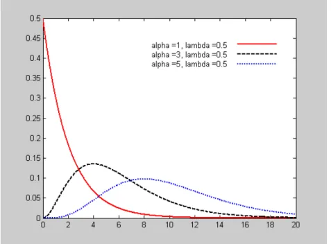
When α = 1, direct integration will verify thatΓ(1)=1, we then get the exponential distribution. Integration by parts will verify that Γ(α +1)=αΓ(α) for any α >1. In particular, when n is a positive integer,Γ(n)=(n−1)!, for example,Γ(6)=120. The gamma distribution is also called the Erlang distribution in this special case. If α is not an integer, Γ(α) can be found approximately by interpolating between the factorials or from tables and software programs. Figure 1(a,b) show the pdf plots for selected combinations of the parameters α and λ. Figure 1a, 1b, 2 are produced using MATLAB.

Figure 1b. Examples of the gamma pdf with fixed α = 3 and various λ

Alternatively, the gamma distribution can be parameterized in terms of a shape parameter α (same as the parameter α in (2.1)) and scale parameter β (equal to 1 / λ in (2.1), λ in (2.1) is the inverse of scale parameter, or sometimes called rate parameter)

(2.3) ( | , )

_{( )}

, 0 , 0, 0 1 > > ∞ < ≤ Γ = − − α β α β β α xα_αe β x x f x

Both (2.1) and (2.3) are commonly used, however (2.1) is the form that will be used through out the paper and also in the attached Java programs.

Cumulative distribution function (cdf)

Gamma distribution does not have a closed form cdf , in other words, its cdf is not expressible in terms of elementary function. When α is not an integer, it is impossible to obtain areas under the density function by direct integration. The best we can do is to express the cdf in terms of

) (α

Γ andγ( xα; ), where γ( xα; )is the “lower” incomplete gamma function defined by (2.4) _{x =}

∫

x_t −_e−t_dt. 0 1 ) ; (α α γ

And the cdf is (Weisstein n.d.)

(2.5)

∫

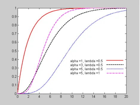
Γ = = xf u du x x F 0 ( ) ) , ( ) ( ) ( α λ α γ

Figure 2. Examples of the gamma cdf

In the special case of α being an integer, there is an important relationship between the gamma and the Poisson distributions, which may simplify the evaluation problem, namely

(2.6) Pr(X ≤ x) = Pr(Y ≥ α) for any x

where Y~Poisson (xλ). (2.6) can be established by successive integration by parts, see Casella and Berger (1990) for details.

The expression (2.5) indicates a potential disadvantage of using gamma distribution, because there may be the need of a numerical algorithm to evaluate the gamma cdf. However, most spreadsheet programs and many statistical and numerical analysis programs have the gamma distribution built in1.

In the unlikely event that only tables are available2, the evaluation problem can be solved by using readily available tables of the distribution and the fact that, if X~gamma (α, λ), then 2λX~ . It generally will be necessary to interpolate in the -table to obtain the desired values (Kaas et al. 2001, p. 36). For example, if X has a gamma distribution with α =1.5 =3/2 and λ = ¼, then 2λX = X/2 has a distribution. Thus, Pr(X < 3.5) = Pr(X/2 < 1.75) can be found by using tables.

2 χ 2 2α χ _χ2 2 3 χ 2 χ

1

Note that in many applications, for example, MS Excel, the parameter λ should be replaced by 1/λ.

Moments & Moment-generating function (mgf) The mgf for a gamma-distributed random variable is

(2.7) . ) 1 ( 1 ) ( 1 ) ( ) ( λ λ α λ α λ α α α < − = ⎥ ⎥ ⎦ ⎤ ⎢ ⎢ ⎣ ⎡ Γ ⎟ ⎠ ⎞ ⎜ ⎝ ⎛ − Γ = for t t t t m .

The reader is referred to Wackely, Mendenhall, and Scheaffer (2002) for a formal derivation. One way of finding the mean and variance of the gamma distribution is to differentiate (2.7) with respect to t and obtain

(2.8) λ α λ λ α α = − = = = + 0 1 ) 1 ( ) 0 ( ' ) ( t t m X E (2.9)

(

)

₂ 0 2 2 0 1 2 ( 1) ) 1 ( ) 1 ( ) 1 ( ) 0 ( '' ) ( λ α α λ α λ α λ λ α α α + = − + = − = = = + = + t t t t dt d m X E (2.10) _{2 2} 2 2 ) 1 ( ) ( λ α λ α λ α α + _{− =} = X V

We can also calculate the moments directly, (2.11) ) ( ) ( ) ( ) ( 0 1 α λ α α λα α λ Γ + Γ = Γ =

_∫

∞ n − − x _n n _x x e _dx n X E Properties

The versatility of the distribution is evident in Figure 1(a,b). When α = 1, the pdf takes its largest value at x = 0, and declines thereafter. For all other values of α, f (x) is zero at x = 0, rises to a maximum and then falls away again. The distribution is obviously not symmetrical. It is positively skewed, but, as α increase, the skewness decreases and the distribution becomes more symmetrical. The sum of n independent gamma random variables, each with pdf (2.1), can be shown to have the gamma distribution with parameters nα and λ. For large n, the Central Limit Theorem tells us that this distribution will be effectively normal with mean nα/λ, and variance nα/λ2 (Hossack, Pollard, and Zehnwirth 1999, p.86)

2.2 Applications in Claim Size Modelling

Gamma distribution as a model for ordinary claims

The Gamma distribution is important as a model for the individual claim size, because it is moderately skewed to the right and has a non-negative range, which is a feature of claim size distributions.

The reader is warned, however that there may be problems with the extreme tail of this distribution, and the issue of the shape of the right-hand tail is a critical one for the actuary. If the gamma distribution is suitable, then we may have obtained a plausible estimate of the tail

probability. If, on the other hand the true underlying pdf fades away to zero more slowly than the gamma, our estimate of the probability will be too low.

Klugman, Panjer, and Willmot (1998) argued that, if the possibility of exceptional large claims were remote, there might be little interest in the purchase of insurance. On the other hand, many loss processes produce large claims with enough regularity to inspire people and companies to purchase insurance and to create problems for the provider of insurance. For any distribution that extends probability to infinity, the issue is one of how quickly the density function approaches zero as the loss approaches infinity. The slower this happens, the more probability is pushed onto higher values and we then say the distribution has a heavy, thicker, or fat tail (p. 85).

Therefore, it is worth reiterating that, when large claims may occur, the tail of the claim size distribution needs special attention. Reinsures in particular need to be cautious not to underestimate the tail. Clearly, a reinsure has the need to fit a “tail” which does not decay away to zero too quickly. Therefore heavy-tailed distribution3, for instance, Pareto distribution, is a more plausible to model if there’re possibilities of extreme large claims. We return to this problem again, in the coming sections.

Klugman, Panjer, and Willmot (1998) have demonstrated how to study the tail behaviour of distributions and distinguish the heavy-tailed distributions from the light-tailed distributions. They also compared the tail weights of Gamma, lognormal and Pareto distributions and found out that Gamma has the lighter tail than the other two (p.86). In general, Gamma distribution is considered by actuaries as a light-tailed distribution and is therefore a reasonable model for small and moderate-sized claims (so-called ordinary or standard claims), that is, for data without large (right-hand) tails. In addition, Gamma distribution has a relatively heavy left-hand tail, which makes it intuitively appealing as the model for small claims.

2.3 Estimation of Parameters

Method of moments v.s. Maximum likelihood estimation (MLE)

We have now determined the gamma family to describe the population of ordinary claims. Our next concern is to determine the values of parameters α, and λ, because the parameters are seldom known a priori. Before the proposed gamma distribution to be applied to any particular actuarial problem, α, λ need to be estimated from claims data.

Statisticians usually choose estimators based on criteria as whether the estimator is unbiased, consistent and efficient. Of the various standard methods, the method of moments is perhaps the oldest and most readily understood, it find estimators of unknown parameters by equating corresponding sample and population moments. However, the MLE, which selects as estimates the values of the parameters that maximize the likelihood of the observed sample, is by far the most popular estimation technique.

The method of moments is sometimes preferred because it’s ease to use and the fact that it sometimes yields estimators with reasonable properties. Unfortunately, moment estimators are

3 _{When we say light-tailed or heavy tailed distributions, we implicitly mean the right-hand tail of the distribution}

consistent but usually not very efficient. In many circumstance, this method yields estimators that may be improved upon, whereas the MLE usually provides estimators, which are quite satisfactory as far as the above criteria are concerned. It is well-known that MLEs have the desirable properties of being consistent, asymptotically normal and asymptotically efficient for large samples under quite general conditions, they are often biased but the bias is generally removable by a simple adjustment.

In some cases, method of moments is a good place to start with. As we will see later, when it is not possible to perform the maximization of likelihood function by analytic means, the method of moments can provide the first approximation for the iterative solution of the likelihood equation. We will demonstrate both methods.

2.3.1. Method of Moments Estimation

Method of moments estimators are obtained by equating the fist k populations moments to the corresponding k sample moments, and solving the resulting system of simultaneous equations. More specifically, they are the solutions of , for k = 1, 2, …t, where is the

kth population moments, ' ' k k =m μ k k =EX ' μ

∑

= = n i k i k X n m 1

' 1 _{the kth sample moments, and t is the number of}

parameters to be estimated.

Suppose we have a random sample of n observations, X1, X2, …, Xn, that is selected from a

population where X_i ~gamma(α,λ) ( i = 1,2,..n). In order to find method of moment

estimators for two parameters α and λ, we must equate two pairs of population and sample moments. The fist two moments of gamma distribution were given in (2.8) and (2.9).

∑

= = = + = = = = n i i X n m X m 1 2 ' 2 2 ' 2 ' 1 ' 1 1 ) 1 ( λ α α μ λ α μ

From the first equation we obtainλˆ =αˆ X . Substituting into the second equation and solving forαˆ , we obtain (2.12) . ) ( ˆ ₂ 2 _{2 2} 2 ₂

∑

∑

− = − = X n X X n X n X X i i α

Substituting αˆ into the first equation yields (2.13)

∑

− = = ˆ _{2 2} ˆ X n X X n X _i α λ

2.3.2 Maximum Likelihood Estimation

As stated above, MLEs are those values of the parameters that maximize the likelihood functionL(x₁,x₂,…x_k |θ₁,θ₂,…θ_k). Clearly, the likelihood function is a function of the

parametersθ₁,θ₂,…,θ_k, we can therefore intuitively write the likelihood function asL(θ₁,θ₂,…θ_k), or sometimes briefly as L.

It is often easier to work with the natural logarithm of , , (known as the log likelihood), than it is to work with directly. This is possible because the log function is strictly increasing on (0, ∞), which implies that the maximum values of and will occur at the same points.

L lnL L

L lnL

Bowman and Shenton (1988) has found out that if X1, .., Xn are independent and identically

distributed as gamma (α, λ), then the MLEs of α and λ are unique but do not have closed-form expressions. Let’s work it out.

Suppose we have a sample of n observations, the likelihood function is then

) ( ) ( ) ( 1 1 1 1 1 1 1 α λ α λ α λ α λ α α λ α α λ α n n x n i i n i i n n x n i i n i x i i i i e x x e x e x L − − = − = − − − = = − − Γ ∑ ⎭ ⎬ ⎫ ⎩ ⎨ ⎧ ⎭ ⎬ ⎫ ⎩ ⎨ ⎧ = Γ ∑ ⎭ ⎬ ⎫ ⎩ ⎨ ⎧ = Γ =

∏

∏

∏

∏

After dropping the uninformative factor , we obtain

1 1 − = ⎭⎬ ⎫ ⎩ ⎨ ⎧

∏

n i i x (2.14) ( ) 1 α λ α λ α n n x n i i i e x L − − = Γ ∑ ⎭ ⎬ ⎫ ⎩ ⎨ ⎧ =

∏

The corresponding log likelihood function of (2.14) is

( )

α

λ

α

λ

α

− + − Γ =

∑

ln

∑

ln ln lnL x_i x_i n n

Taking partial derivatives with respect to α, λ and setting to zero we obtain,

(2.15) ln ln ln ln ( )⎟=0 ⎠ ⎞ ⎜ ⎝ ⎛ _Γ − + = ∂ ∂

_∑

a d d n n x L i λ _α α (2.16) ln =− + =0 ∂ ∂

_∑

λ α λ n x L i .

(2.15), (2.16) are called the likelihood equations, or sometimes normal equations. Solving (2.16) for λ gives

(2.17) x x n x_{i α} λ α α λ =

∑

= ⇒ = 1

Where α, are the MLEs of α and λ respectively and λ x =

∑

x_i n= sample mean, and (2.15) then turns into

(2.18) lnx+lnα −lnx−ψ(α)=0 Where lnx=

(

∑

lnx_i

)

n and ( ) ln (a) d d _Γ = α α

ψ (the logarithmic derivative of the gamma function) is called the digamma function.

It is readily seen that the system of equations (2.15) and (2.16) can not be solved analytically because of the digamma and logarithm functions; therefore we have confirmed that the MLEs do not have a closed form. They are, however, indeed unique. And to obtain them, numerical methods must be applied. We may first determine αˆ using an iterative search like Newton-Raphson method, αˆ is then substituted into (2.17) to determine , as will be demonstrated in the following example.

λˆ A Numerical Example-Newton-Raphson method4

Suppose we have a sample known to come from gamma (2, 0.5), each value of which was obtained by adding four consecutive entries from a table of realizations of 2 variables

1

χ 5_{. The}

sample is as follows:

Table 1. A sample of gamma (2,0.5) distributed random numbers

5.6135 2.2197 5.8971 3.8243 6.5021 0.8590 3.5452 2.4983 2.0567 0.7797 1.0184 11.3595 2.1279 2.0924 4.1648 4.9673 0.3939 4.7217 2.9399 6.8468 5.6229 3.6467 6.0812 1.9336 4.4899 2438 . 0 ln ln 3475 . 1 ln , 702 . 20 , 8477 . 3 , 1037 . 1 ln 5038 .. 517 , 1934 . 96 , 59314 . 27 ln 2 2 = − = = = = = = =

∑

∑

∑

x x x x x x x x x

For this sample, given thatlnx− xln =0.2438, (2.18) turns into (2.19) 0h(α)=lnα −ψ(α)−0.2438=

4 _{This example is adapted from Handbook of applicable mathematics, pp 316-318}

5 _{Recall in (2.1) we stated that the sum of n independent gamma (α, λ) variables distribution gamma (nα, λ), since}

is essentially gamma (0.5, 0.5), sum of 4 independent variables will have gamma (2, 0.5). 2

1

χ 2

1

We first solve (2.19) forα , then put the resulting expression into (2.17) and obtain 8477 . 3 ˆ α λ =

As discussed before, we can use the method of moment’s estimates as the first approximation, which are obtained using (2.12) and (2.13)

52 . 2 ˆ ₂ 2 ₂ = − =

∑

x nx x n i α , ˆ _{2 2} =0.65 − =

∑

x nx x n i λ

Now we have the first approximations for the iterative solution of the likelihood equations (2.15) and (16).

We will use the Newton-Raphson method. The formula is (2.20) ) ( ' ) ( 1 n n n n x h x h x x + = −

(See Adams and Robert 2003, p.273)

Applying (2.20), the iteration proceeds as follows,

Table 2. Solving the likelihood equation of gamma distribution using Newton-Raphson method

Iteration No. α ψ(α) h(α) Ψ´(α) H´(α) Correction ( -h(α)/h´(α))

1 2.52 0.713 -0.32 0.49 -0.09 -0.36

2 2.160 0.521 0.0052 0.590 -0.123 0.042

3 2.202 0.5454 0.00013 0.5723 -0.1182 0.0011

4 2.203

Thus,αˆ =2.203, whence , which are quite satisfactory results. They are also closer to the true values (α = 2, λ = 0.5) comparing to the method of moments estimates.

573 . 0 ˆ =

λ

In the above computations, ψ(α) is the digamma function, ψ´(α) is its 1st derivative, known as the trigamma function, the nth derivative of ψ(α) is called the polygamma function, denoted as

) (α

ψn _{. Those functions can be evaluated in relatively math-specialized software programs, for}

example, in Mathematica, ψ(α) is returned by the function PolyGamma [z] or PolyGamma [0, z], )

(α

ψn _{is implemented as}

PolyGamma [n, z]. Approximating MLEs in closed-form

Alternatively, ψ(α) can be approximated, very accurately using the following Equation (see Shorack 2000, p.548). (2.21) ... 240 1 252 1 120 1 12 1 2 1 ln ) ( _{2 4 6 8} α α α α α α α ψ = − − + − + ,

Taking the first derivative of (2.21) yields (2.22) = + ₂ + ₃ − ₅ + ₇ − ₉ − 30 1 42 1 30 1 6 1 2 1 1 ) ( ' α α α α α α ψ z

Hory and Martin (2002) have used approximated ψ(α) in (2.21) to the first three terms, and in this way they derived an analytical approximation to the solutions of the likelihood equations system (2.15), (2.16). Their resulting (approximating) MLE estimators (in closed-form) are

(2.23)

(

)

(

)

(

)

(

2 1

)

2 1 2 1 2 1 2 ) ln( 4 3 ) ln( 4 1 1 ˆ ) ln( 4 3 ) ln( 4 1 1 ˆ u u u u u u u u u − − + + = − − + + = λ α where x u₁ =ln , u₂ = x

We can apply (2.23) directly for our numerical example and obtain an approximation of MLEs,

(

)

(

)

(

)

(

ln(3.8477) 1.1037

)

0.573 ) 8477 . 3 ( 4 3 1037 . 1 ) 8477 . 3 ln( 4 1 1 ˆ 206 . 2 1037 . 1 ) 8477 . 3 ln( 4 3 1037 . 1 ) 8477 . 3 ln( 4 1 1 ˆ = − − + + = = − − + + = λ α

In this case, the approximation is very satisfactory. In general, Hory and Martin (2002)’s study has shown that (2.23) often leads to slightly over-estimated parameters.

3. The Reciprocal Gamma Distribution

3.1 Definition, Moments & Properties of the Distribution

Probability density function (pdf)

The random variable Y 1= X is reciprocal gamma (R-gamma) distributed if X is gamma distributed. Its pdf can be derived from (2.1) the gamma pdf by defining the transformation

X X g Y = ( )=1 .

(

)

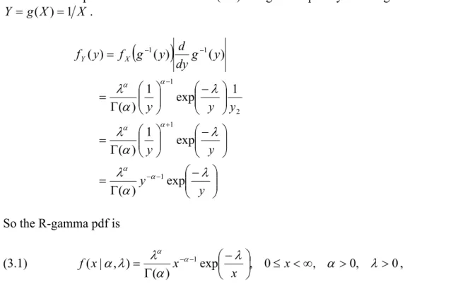
⎟⎟ ⎠ ⎞ ⎜⎜ ⎝ ⎛ − Γ = ⎟⎟ ⎠ ⎞ ⎜⎜ ⎝ ⎛ − ⎟⎟ ⎠ ⎞ ⎜⎜ ⎝ ⎛ Γ = ⎟⎟ ⎠ ⎞ ⎜⎜ ⎝ ⎛ − ⎟⎟ ⎠ ⎞ ⎜⎜ ⎝ ⎛ Γ = = − − + − − − y y y y y y y y g dy d y g f y f_{Y X} λ α λ λ α λ λ α λ α α α α α α exp ) ( exp 1 ) ( 1 exp 1 ) ( ) ( ) ( ) ( 1 1 2 1 1 1 So the R-gamma pdf is (3.1) exp , 0 , 0, 0 ) ( ) , | ( 1 _{⎟ ≤ <∞ > >} ⎠ ⎞ ⎜ ⎝ ⎛ − Γ = − − λ _{α λ} α λ λ α α α _x x x x f ,

where α is known as the shape parameter, and λ the scale parameter.

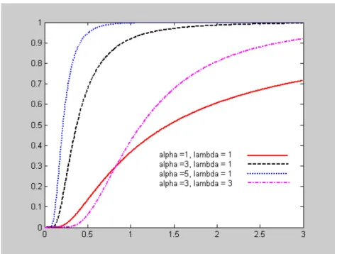
Figure 3 (a, b) shows the pdf plots for selected combinations of the parameters α and λ. Figure 3a, 3b and 4 are produced using MATLAB.

Figure 3a. Examples of the R-gamma pdf with fixed λ = 1 and various α

Figure 3b. Examples of the R-gamma pdf with fixed α = 3 and various λ

Cumulative distribution function (cdf)

The cdf of R-gamma can be expressed in terms of Γ(α)andΓ( xα; ), where Γ( xα; )is the “upper” incomplete gamma function defined by

(3.2) Γ =

∫

∞ − − . x t_dt e t x₎ 1 ; (α α

Note that by definition, the lower and upper incomplete gamma functions satisfy ) ( ) , ( ) ; (α +γ α =Γα Γ x x And the cdf is (3.3)

( )

) ( ) , ( ) ( ) 1 , ( 1 ) , | 1 ( 1 ) , | ( α λ α α λ α γ λ α λ α Γ Γ = Γ − = − = F x x x x F Since,F(x|α,λ)=P(X ≤x)=P(1 X >1x)=1−F(1 x|α,λ),

Figure 4. Examples of the R-gamma cdf

Moments

The moments of the reciprocal gamma distribution are

(3.4) , 0 ) ( ) ( exp ) ( ) ( 0 1 _{− >} Γ − Γ = ⎟ ⎠ ⎞ ⎜ ⎝ ⎛ − Γ =

∫

∞ − − _dx n _n x x x X E n n n _α α α λ λ α λα α _.

We can find the mean, and variance of R-gamma distribution through (3.4),

(3.5) , 1 1 ) ( > − = α α λ X E (3.6) , 2 ) 1 )( 2 ( ) ( 2 2 _> − − = α α α λ X E

(3.7) , 2 ) 1 )( 2 ( ) 1 ( ) 1 )( 2 ( ) ( ₂ 2 2 2 2 > − − = − − − − = α α α λ α λ α α λ X V

3.2 Applications in Claim Size Modelling

Reciprocal gamma as a model for extremely large claims

In 2.2, we discussed that gamma distribution is a suitable model for small and moderate claims because of its plausible shape and its light-tail. However, in several lines of insurance business extremely large claims occur, and in recent years actuaries have become more and more aware of the potential risk inherent in large claim sizes. Studies have shown that heavy-tailed distributions needed to be used for modelling large claims. Unlike the gamma distribution, few existing literature studied the tail behaviour of R-gamma, therefore it is worth explaining here.

For heavy-tailed distributions, the survival function,

∫

∞ = − = x f t dt x F x S( ) 1 ( ) ( )

which gives the probability of loss exceeding the value x, have (relatively) large values of S(x) for given x. Also the pdf itself can be used to test tail behaviour. For some distributions, S(x) and/or f(x) are simple functions of x and we can immediately determine what the tail looks like. If they are complex functions of x, we may be able to obtain a simple function that has similar behaviour as x gets large. We use the notation

∞ → x x b x a( )~ ( ), to mean lim_x→∞a(x) b(x)=1

(Klugman, Panjer, and Willmot 1998, p86)

Therefore, as x gets large, the R-gamma pdf given in (3.1) can be denoted by

(3.8) →∞ Γ − − _x x x f , ) ( ~ ) , | ( α α 1 α λ λ α

Clearly, the tail of the R-gamma pdf for large x values is a power-law with exponent (-α-1). Since power tail is special case of heavy tail. R-gamma is a heavy-tailed distribution and thus a reasonable model for large claims. The parameter α in (3.8) controls the power-law decay for large x values. Intuitively, since we already know that the gamma distribution has a light right tail and heavy left hand tail; by taking its reciprocal we essentially mapped the left tail into the right tail.

3.3 Estimation of Parameters

3.3.1 Method of Moments Estimation

Suppose we have a random sample of n observations, Y1, Y2,…Yn, that is selected from a

distribution were given in (3.5) and (3.6), equating them to the corresponding sample moments gives, 1 , 1 ' 1 ' 1 =_{α −} = = α > λ μ m Y 2 , 1 ) 1 )( 2 ( 1 2 ' 2 2 ' 2 = _{− −} = =

∑

> = α α α λ μ n i i Y n m .

Solving for α and λ in terms of the first two moments yields

(3.9) _{2 2} 2 2 2 2 2 ˆ , 2 ˆ Y n Y Y Y Y n Y Y n Y i i i i − = − − =

∑

∑

∑

∑

λ α .

3.3.2 Maximum Likelihood Estimation

From the R-gamma pdf (3.1), we can derive the likelihood function of α, λ on the above sample of n observations, which is (3.10) ) ( 1 ) ( ) ( 1 1 1 1 1 1 1 1 1 α λ α λ α λ α λ α α λ α λ α α n n y n i i n i i n n y n i i n i y i i i e y y e y e y L − − = − = − − − − = = − − − Γ ∑ ⎭ ⎬ ⎫ ⎩ ⎨ ⎧ ⎭ ⎬ ⎫ ⎩ ⎨ ⎧ = Γ ∑ ⎭ ⎬ ⎫ ⎩ ⎨ ⎧ = Γ =

∏

∏

∏

∏

After dropping the uninformative factor , if we set

1 1 − = ⎭⎬ ⎫ ⎩ ⎨ ⎧

∏

n i i y n i x y_{i i}, 1,2, 1 = = ,

it is readily seen that the resulting likelihood function coincides with the gamma counterpart (2.14).

Therefore, it follows that the MLE analysis of R-gamma distribution is carried out by replacing each observation by its reciprocal y_i x_i =1 y_i and proceeding as for the Gamma distribution. Similarly, as the R-gamma version of (2.23), the approximating MLEs for R-gamma are obtained by defining u₁ =ln

( )

1 y and u₂ =1 y

(3.11)

(

)

(

)

(

)

(

2 1

)

2 1 2 1 2 1 2 ) ln( 4 3 ) ln( 4 1 1 ˆ ) ln( 4 3 ) ln( 4 1 1 ˆ u u u u u u u u u − − + + = − − + + = λ α where u₁ =ln

( )

1 y , u₂ =1 y.

4. The Mixture of Gamma & Reciprocal Gamma

4.1 The Mixture of Gamma & Reciprocal Gamma

Mixture of gamma & R-gamma as a model for heterogeneous portfolio

In section 2, we proposed the gamma distribution as the model for ordinary claim sizes; in section 3, the reciprocal gamma was introduced to model extra large claim sizes. Very often, the insurance portfolio is heterogeneous in the sense that, in addition to a large number of “ordinary” policies, it also contains a small number of policies under which much larger claim sizes are likely (Hossack, Pollard, and Zehnwirth 1999, p.256).

Klugman, Panjer, and Willmot (1998) have presented an example of heterogeneous portfolio- a hospital’s general liability coverage. In this case, one process is carelessness in patient handling, which would include lost items such as dentures and eyeglasses as well as small incidents such as wheel chair collisions. The other process takes place in the operating room, where surgeons may create events with costly consequences. (p.105).

Under those circumstances, the population of claims consist of two components (groups), G1,

and G2, corresponding to ordinary and extra large claims. If we could not separate the data into

these two components we can not model them separately. Following our previous discussion on gamma, and R-gamma’s applications in claim size modelling, when there’s a mixture of ordinary and large claims, it is intuitively appealing to use a mixture of gamma and R-gamma model.

The pdf for the mixture is simply the weighted sum of gamma (α1, λ1) and R-gamma (α2, λ2)

(for an introduction to mixture distributions see Titterington et al. 1985),

(4.1) ⎟ ⎠ ⎞ ⎜ ⎝ ⎛ − Γ − + Γ = − − − − x x p e x p p x f x 1 2 2 2 1 1 1 2 2 1 1, , , , ) _{( )} (1 ) _{( )} exp | ( 2 2 1 1 1 λ α λ α λ λ α λ α α α λ α α . ) 1 0 ( < p<

The weights are the proportions (p and 1-p) of ordinary claims and extra large claims respectively. From another point of view, p is the probability that a particular claim falls into the component G1 (ordinary claims), and 1-p is for G2 (extra large claims). The gamma &

R-gamma mixture thus has five parameters, α1, λ1, α2, λ2, and the so-called mixing parameter p.

In this mixture model, the gamma distribution has a lighter tail. This might be a model for the frequent, small claims while the R-gamma distribution covers the large, but infrequent claims. The previously discussed single gamma and single R-gamma models can be seen as the special cases of the general mixture model at p = 1, and p = 0.

Mean, Variance & Moments

Denote f₁(x)as the gamma density with meanμ₁ and varianceσ₁, and the R-gamma with ) ( 2 x f 2

(4.2) f(x)= pf₁(x)+(1− p)f₂(x). The moments of mixture distribution f(x)satisfy

(4.3)

[

]

, ) 1 ( ) ( ) 1 ( ) ( ) ( ) 1 ( ) ( ) ( ) ( ' 2 1 ' 2 1 2 1 n n n n n n n p p dx x f x p dy x f x p dx x f p x pf x dy x f x X E μ μ + − = − + = − + = =

∫

∫

∫

∫

∞ ∞ − ∞ ∞ − ∞ ∞ − ∞ ∞ −

where is the nth moment of the gamma distribution, and the R-gamma. Formula (4.3) is a useful tool when we apply the moment estimation in the next section.

1 ' n μ ' 2 n μ

From (4.3) and the relation ( 2)₌ 2 ₊ 2, ₌1,2. It is easy to verify that, i X E _i μ_i σ_i (4.4) E(Y)= pμ₁ +(1−p)μ₂,

[

]

2. 2 1 2 2 2 1 (1 ) (1 ) ) (Y = pσ + − pσ + p − p μ −μ V

4.2 Estimation of Parameters in the Gamma-Reciprocal Gamma Mixture

4.2.1 Method of Moments Estimation

In the mixture model (4.1), there are five parameters overall, namely α1, λ1, α2, λ2, and p.

Therefore we must equate five pairs of population and sample moments, provided that first 5th

moments are available (α₂ >5). Formulas of moments for single gamma and R-gamma are given in (2.11) and (3.4), applying also (4.3), we can establish the first five moments for (4.1) and then equate them to the first 5 sample moments.

A simplified case with known α1 and α2 (> 3)

To present the idea, we consider a simplified case when the α1 and α2 (> 3)are already known a

priori, so there’re then only 3 parameters to be estimated.

(4.5)

( )

( )

( )

⎪ ⎪ ⎪ ⎪ ⎩ ⎪⎪ ⎪ ⎪ ⎨ ⎧ = − − − − + + + = = − − − + + = = − − + = ' 3 2 2 2 3 2 3 1 1 1 1 ' 2 ' 2 2 2 2 2 2 1 1 1 ' 2 ' 1 2 2 1 1 ' 1 ) 1 )( 2 )( 3 ( ) 1 ( ) 1 )( 2 ( ) 1 )( 2 ( ) 1 ( ) 1 ( 1 ) 1 ( m p p m p p m p p α α α λ λ α α α μ α α λ λ α α μ α λ λ α μ

What is shown above is a system of three non-linear simultaneous equations, which must be solved to give the estimates of the unknown three parameters p, λ1, and λ2. It is obvious that even for this simplified case the algebra can be very heavy. The solution can be accomplished by some numerical method, for example, the Newton-Raphson method. We have introduced in details the Newton-Raphson method for one equation in one unknown in section 2.3.2. As we

will see, this method can be easily extended to finding solutions of systems of m equations in m variables. The process goes as follows, with the iterations stops when the desired accuracy has been achieved.

1. For one single equation f(x) = 0, we do iteration _xn _→xn+1 following

) ( ' ) ( 1 n n n n x f x f x x + = − _.

This is the formula we used in section 2.3.2 (formula (2.20)). x0 should be chosen suitably

close to x.

2. System with m equations and m unknowns.

or in vector form m i x x f_i( ₁,…, _m)=0, =1,… f (x) = 0.

Let vector x = [x1,…xm], Iteration xn →xn+1 by solving the following linear system

0 x f x x x J₍ n₎₍ n+1− n₎+ ₍ n₎= (4.6) , _xn+1 _=xn _−J(_xn)−1_f(_xn) where is the Jacobian matrix defined as, J(x)

⎥ ⎥ ⎥ ⎥ ⎥ ⎦ ⎤ ⎢ ⎢ ⎢ ⎢ ⎢ ⎣ ⎡ ∂ ∂ ∂ ∂ ∂ ∂ ∂ ∂ = ⎟ ⎟ ⎠ ⎞ ⎜ ⎜ ⎝ ⎛ ∂ ∂ m m m m j i x f x f x f x f x f 1 1 1 1

We will denote the determinant of Jacobian matrix as J,

m m m m j i x f x f x f x f x f J ∂ ∂ ∂ ∂ ∂ ∂ ∂ ∂ = ⎟ ⎟ ⎠ ⎞ ⎜ ⎜ ⎝ ⎛ ∂ ∂ = 1 1 1 1 det

⎪ ⎪ ⎪ ⎪ ⎩ ⎪⎪ ⎪ ⎪ ⎨ ⎧ = − − − − − + + + = = − − − − + + = = − − − + = . 0 ) 1 )( 2 )( 3 ( ) 1 ( ) 1 )( 2 ( 0 ) 1 )( 2 ( ) 1 ( ) 1 ( 0 1 ) 1 ( ' 3 2 2 2 3 2 3 1 1 1 1 ' 2 2 2 2 2 2 1 1 1 ' 1 2 2 1 1 m p p h m p p g m p p f α α α λ λ α α α α α λ λ α α α λ λ α

The vector of unknowns is x=[p,λ₁,λ₂], and the Jacobian matrix is given by

⎥ ⎥ ⎥ ⎥ ⎥ ⎥ ⎥ ⎦ ⎤ ⎢ ⎢ ⎢ ⎢ ⎢ ⎢ ⎢ ⎣ ⎡ ∂ ∂ ∂ ∂ ∂ ∂ ∂ ∂ ∂ ∂ ∂ ∂ ∂ ∂ ∂ ∂ ∂ ∂ = 2 1 2 1 2 1 2 1, ) , ( λ λ λ λ λ λ λ λ h h p h g g p g f f p f p J where,

(

)

(

)(

)

(

)

(

)(

)

(

)(

)

(

)(

)(

)

(

)(

)

(

3

)(

2

)(

1

)

. ) 1 ( 3 1 2 3 1 2 3 1 2 1 2 ) 1 ( 2 1 2 1 2 1 1 1 ) 1 ( 1 2 2 2 2 2 2 4 1 1 1 1 1 2 2 2 2 2 3 1 1 1 1 2 2 2 2 3 1 1 1 1 2 2 2 2 2 1 1 1 2 2 2 1 1 1 2 2 1 1 − − − − = ∂ ∂ + + − = ∂ ∂ − − − − + + = ∂ ∂ − − − = ∂ ∂ + − = ∂ ∂ − − − + = ∂ ∂ − − = ∂ ∂ − = ∂ ∂ − − = ∂ ∂ α α α λ λ λ α α α λ α α α λ λ α α α α α λ λ λ α α λ α α λ λ α α α λ λ α λ α λ λ α p h p h p h p g p g p g p f p f p f

Having chosen a suitable vector of starting values , formula (4.6) is applied to successively find the next x values until convergence. We can solve (4.6) by either directly

taking the inverse of the Jacobian matrix, or use the Cramer’s rule, which yields, ] , , [ 0 ₁0 ₂0 0 _{= p λ λ} x

) , , ( ) , , ( ) , , ( 2 1 2 1 2 1 2 1 2 1 2 2 1 3 1 3 1 3 1 1 1 1 2 1 3 2 3 2 3 2 1 n n n n n n n n n n n n n n n p J h h h g g g f f f p J h h h g g g f f f p J h h h g g g f f f p p λ λ λ λ λ λ λ λ λ λ − = − = − = + + + where , , , 2 3 1 2 1 _{λ ∂λ} ∂ = ∂ ∂ = ∂ ∂ = f f f f p f

f J, as said above, is the determinant of the Jacobian matrix. The method of Cramer’s rule is used in the Java Mixture Model Estimation Program, see Appendix E: Java source code- Newton_Solver.java.

In general, using Newton-Raphson method, convergence is not always guaranteed for a certain system of equations. Therefore to check whether Newton-Raphson method works well for system (4.5), we can test in the following numerical example.

Example: Suppose we know, α1=2, λ1= 1, α2= 4, λ2= 60, p =0.9, the corresponding population

moments are therefore μ1=3.8, μ2= 65.4, μ3= 3621.6 (calculated by (4.3) or (4.5)).

If we let m1, m2, m3 equal to u1, u2, u3, the solutions of p, λ1, λ2 should be exactly their true

values 0.9, 1, 60. We now can test Newton-Raphson method by solving (4.5) for p, λ1, λ2 and

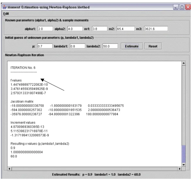
then comparing to their true values. The Java Mixture Model Estimation Program is an ideal tool for this purpose. The results can be achieved in one second. A complete users’ guide of the program is given in Appendix B.

Our inputs are α1=2, α2= 4, m1 (= μ1) =3.8, m2 (= μ2) =65.4, m3 (= μ3) = 3621.6. The starting

values are chosen as . The output is shown in the following

graph. ] 50 , 8 . 0 , 7 . 0 [ ] , , [ 0 ₁0 ₂0 0 _{= p λ λ =} x

Figure 5. Applying the Newton-Raphson method-an example

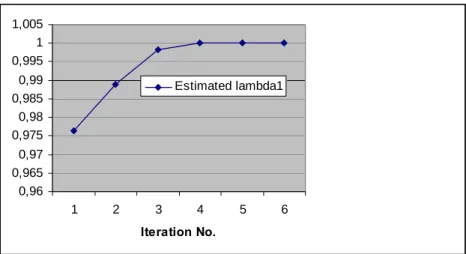
The convergence is very fast, after six iterations we get the expected results. We can record the estimated values for every iteration and plot in Excel, see Figure 6 (a,b,c). Experiments show that it is same effective if we use slightly “poorer” starting values.

Figure 6a. Convergence of p

0,89 0,895 0,9 0,905 0,91 0,915 0,92 1 2 3 4 5 6 Iteration No. p Estimated p

Figure 6b. Convergence of λ1 0,96 0,965 0,97 0,975 0,98 0,985 0,99 0,995 1 1,005 1 2 3 4 5 6 Iteration No. Estimated lambda1 Figure 6c. Convergence of λ2 50 52 54 56 58 60 62 64 1 2 3 4 5 6 Iteration No. Estimated lambda2

We can try more examples with various parameters, for example, we may worry whether Newton-Raphson method works well for the cases where the mean of the reciprocal gamma component is much larger than the gamma component, or the cases where p is almost 1 (so weight of the reciprocal gamma component is almost zero). The results of those experiments shows that Newton-Raphson method is a good choice, the convergence almost always happens within 15 iterations.

Therefore, it is reasonable to hope that if the sample moments are good approximations of the population moments, our moment estimation algorithm will provide satisfactory estimation for the unknown parameters p, λ1, λ2, given α1, and α2 > 3. In section 5, we will simulate samples

of the mixture model using the Java Mixture Model Simulation Program, and then evaluate our moment estimation algorithm (for the simplified case) using the Java Mixture Model Estimation Program.

4.2.2 Maximum Likelihood Estimation

As discussed previously, MLEs are well known to have desirable asymptotic properties and it is natural to consider the method for estimating the parameters in our mixture model (4.1). (For an introduction of MLE method for mixture distributions, see Everitt and Hand 1981 or McLachlan and Peel 2000). Unfortunately, in practice for our mixture model the MLE is more difficult and time-consuming to apply than the moment estimation. However, it is rather simple to theoretically derive the solution concept of this method.

The likelihood function is given by

[

]

∏

∏

= = − + = = n i i i n i i p pf x p f x x f L 1 2 2 2 1 1 1 1 2 2 1 1, , , ) ( | , ) (1 ) ( | , ) , | ( α λ α λ α λ α λ

where f(x_i | p,α₁,λ₁,α₂,λ₂) denotes the mixture distribution (4.1), and

i x i i x e x f 1 1 1 1 1 1 1 1 1 ) ( ) , | ( α λ α α λ λ α − − Γ = is the gamma component, and

⎟ ⎠ ⎞ ⎜ ⎝ ⎛ − Γ = − − x x x f _i 1 2 2 2 2 2 2 exp ) ( ) , | ( 2 2 λ α λ λ α α α

the R-gamma component.

The corresponding log likelihood function is

(4.7)

∏

∑

[

]

= = − + = = n i i i n i i p pf x p f x x f L 1 1 1 1 2 2 2 1 2 2 1 1, , , ) ln ( | , ) (1 ) ( | , ) , | ( ln ln α λ α λ α λ α λ

The likelihood equations, which are obtained by equating the first partial derivatives of (4.7) with respect to p, α1, λ1, α2, λ2, to zero, are given by

(4.8) ( ( | , ) ( | , )) 0 ) , , , , | ( 1 ln 2 2 2 1 1 1 1 1 1 2 2 = − = ∂ ∂

_∑

= λ α λ α λ α λ α i i n i i x f x f p x f p L (4.9) 0 ) , , , , | ( ) , | ( ln 1 1 1 2 2 1 1 1 1 1 = ∂ ∂ = ∂ ∂

∑

= n i i i p x f x f p L λ α λ α α λ α α (4.10) 0 ) , , , , | ( ) , | ( ln 1 1 1 2 2 1 1 1 1 1 = ∂ ∂ = ∂ ∂

∑

= n i i i p x f x f p L λ α λ α λ λ α λ (4.11) 0 ) , , , , | ( ) , | ( ) 1 ( ln 1 1 1 2 2 2 2 2 2 2 = ∂ ∂ − = ∂ ∂

∑

= n i i i p x f x f p L λ α λ α α λ α α (4.12) 0 ) , , , , | ( ) , | ( ) 1 ( ln 1 1 1 2 2 2 2 2 2 2 = ∂ ∂ − = ∂ ∂

_∑

= n i i i p x f x f p L λ α λ α λ λ α λ

As the gamma component is assumed to exist in a fixed proportion p in the mixture (and the R-gamma in (1-p)), we may talk about the probability that a particular observation belongs to one of the component. By Bayes Rule, the probability that a given comes from the gamma component is i x i x (4.13) ) , , , , | ( ) , | ( ) | Pr( 2 2 1 1 1 1 1 λ α λ α λ α p x f x pf x gamma component i i i = ,

For convenience, we will sometimes use f(x_i), f₁(x_i), f₂(x_i) as shortened notations for ) , , , , | (x pα₁ λ₁ α₂ λ₂ f _i ,f₁(x_i |α₁,λ₁), f₂(x_i |α λ₂, ₂). If we manipulate (4.8), an interesting result n

x f x f n i i i ₌

∑

=1 2 ) ( ) (

can be obtained, as follows. First multiply (4.8) by p, (4.14) ( ( ) ( ) 0 ) ( 1 2 1 = −

∑

= i i n i i x f x f x f p

Using the fact that, f(x)= pf₁(x)+(1− p)f₂(x)⇒ pf₁(x)− pf₂(x)= f(x)− f₂(x), (4.14) can be written as 0 ) ( ) ( 0 ) ( ) ( 1 0 ) ( ) ( ) ( 1 2 1 2 1 2 = − ⎟⎟ ⎠ ⎞ ⎜⎜ ⎝ ⎛ = ⎟⎟ ⎠ ⎞ ⎜⎜ ⎝ ⎛ − = −

∑

∑

∑

= = = n x f x f x f x f x f x f x f n i i i n i i i n i i i i (4.15) n x f x f n i i i ₌

∑

=1 2 ) ( ) (

Now we multiply (4.8) by p again, the purpose of which is to write its solution in terms ofPr(component gamma|x_i). ⇒ = − = − = ⎟⎟ ⎠ ⎞ ⎜⎜ ⎝ ⎛ − = −

∑

∑

∑

∑

∑

= = = = = ) 15 . 4 ( ), 13 . 4 ( 0 ) | Pr( 0 ) ( ) ( ) ( ) ( 0 ) ( ) ( ) ( ) ( 0 ) ( ) ( ( ) ( 1 1 2 1 1 1 2 1 2 1 1 ∵ np x gamma component x f x f p x f x pf x f x pf x f x pf x f x f x f p n i i n i i i n i i i n i i i i i i i n i i

(4.16)

∑

= = n i i x gamma component n p 1 ) | Pr( 1 ˆ

Also, using (4.13) in (4.9)-(4.12), we can express them as

(4.17) Pr( | ) ln ( | , ) 0 1 1 1 1 1 ₌ ∂ ∂

∑

= n i i i x f x gamma component α λ α (4.18) Pr( | ) ln ( | , ) 0 1 1 1 1 1 ₌ ∂ ∂

∑

= n i i i x f x gamma component λ λ α (4.19) Pr( | ) ln ( | , ) 0 1 2 2 2 2 ₌ ∂ ∂ −

∑

= n i i i x f x gamma R component α λ α (4.20) Pr( | ) ln ( | , ) 0 1 2 2 2 2 ₌ ∂ ∂ −

∑

= n i i i x f x gamma R component λ λ α

Note that Pr(component R−gamma|x_i)=1−Pr(component gamma|x_i)

The forms in (4.17)-(4.20) are intuitively attractive. The likelihood equations for estimating α1,

λ1, α2, λ2 are weighted averages of the likelihood equations arising from of gamma or R-gamma

considered separately. The weights are the probabilities of membership of each sample point in each class.

i

x

Of course equations (4.16)-(4.20) do not give the estimators analytically, instead they must be solved using some type of iterative procedure, for instance, EM algorithm (see McLachlan et al 2000). The simplest way is a method (see Everitt, 1981) that is essentially an application of the EM algorithm. Applying this method we first find initial values of the parameters (obtained by some other methods or simply by experience), then insert them into (4.13) to obtain the first estimates of , this is then inserted into equation (4.16) to (4.20) to give revised parameter estimates and the process is continued until convergence.

) | Pr(component gamma x_i

5. Simulation Studies

5.1 Simulation

Based on our gamma & R-gamma mixture model (or the single gamma and single R-gamma models as two special cases), a Java Mixture Model Simulation Program is specially designed for the simulation purpose. A complete users’ guide of the program is given in Appendix A. All the figures in this section are produced by the program.

The basic idea of the simulation for our model is straightforward, we simulate random numbers that either follow a gamma (α1, λ1) distribution (with probability p), or R-gamma (α2, λ2)

distribution (1-p). To generate a random observation on the R-gamma distribution, all one has to do is to generate a random observation on the corresponding gamma distribution and take the reciprocal of the result.

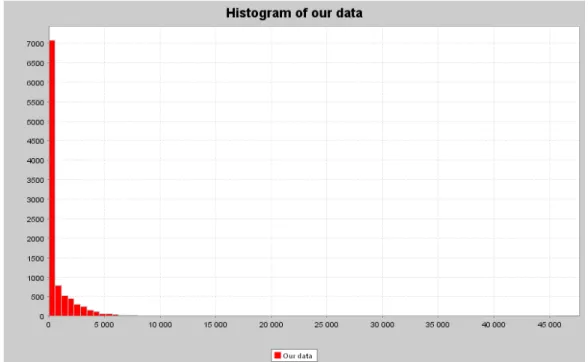
Since the mean of the gamma component is supposed to be much smaller than the mean of the R-gamma component6, a general (normal) histogram do not look very illustrative, especially when p is close to one, as shown in Figure 7.

Figure 7. General histogram of 10,000 random observations on the mixture model

α1 = 3.0; λ1 = 0.01; α2 = 3.0; λ2 = 6000 and p = 0.75

A better alternative is to produce the histograms in logarithmic scale. Figure 8 (a, b, c) presents log histograms for different values of parameters α1, λ1, α2, λ2, and p.

6 _{This is because in the mixture model the gamma component covers the claims that are much smaller than what}

Figure 8. Log histograms of 10,000 random observations on the mixture model

(a) α1 = 3.0; λ1 = 0.01; α2 = 3.0; λ2 = 60000 and p = 0.9

(c) α1 = 3.0; λ1 = 0.01; α2 = 3.0; λ2 = 6000 and p = 0.75

Figure 8 (a,b,c) illustrate how our mixture of gamma and reciprocal gamma model can create a bi-modal distribution.

5.2 Estimation

This section is aimed to evaluate the method of moment estimation we derived in section 4.2.1. Our goal is therefore limited to the simplified case where α1, α2>3 are known. The evaluation

proceeds as follows: first we use the Java simulation program to simulate samples (the parameters α1, α2, λ1, λ2 and p are chosen by us) and computes the first three sample moments

(m1, m2, m3) for each sample; we will generate 20 samples each for sample sizes (n) of 100,

200, 500 and 1000. Next we take the average m1, m2, m3 of the 20 samples for n =100, 200,

500 and1000. Finally we use the Java estimation program to estimate p, λ1, and λ2 (and

compare to their true values) for each sample size n given α1, α2 and the corresponding average

m1, m2, m3.

In our mixture model, the reciprocal gamma component is supposed to have larger mean than the gamma component, and the weight (1-p) of reciprocal gamma is reasonably assumed to be very small, i.e. 0.1 or 0.05. We will therefore focus on such cases.

Case One: Samples generated by the following parameters

α1 = 2.0; α2 = 4.0; p = 0.9; λ1 = 1 and λ2 = 60

The means of the gamma and the R-gamma components are therefore 2 and 20 respectively.

Table 3. Results (m1, m2, m3) of the Java Mixture Model Simulation Program (for case 1 )

n = 100 n = 200

Sample No. m1 m2 m3 Sample No. m1 m2 m3

1 3,3566 46,1222 1461,0833 1 3,4795 45,1929 1222,5706 2 3,6025 44,2636 984,0578 2 3,3594 40,7412 874,1341 3 3,5380 49,3988 1179,8444 3 3,6581 52,8973 1574,8707 4 3,1809 32,0837 568,4237 4 3,1864 29,7927 482,3741 5 3,6396 61,3733 2208,3176 5 3,6409 43,6022 1004,6762 6 3,6767 44,4214 941,4238 6 3,6889 47,9849 1324,5586 7 3,1150 31,0644 560,2580 7 4,0897 80,4335 3933,2784 8 3,2579 28,5210 404,4903 8 3,4122 44,5275 1185,9261 9 3,5199 51,7304 1476,0766 9 4,8066 156,0900 11117,1673 10 3,7619 35,4741 533,2758 10 3,8587 49,1643 1178,9222 11 3,4535 44,2780 1397,3511 11 2,9903 29,6945 610,0595 12 3,9242 51,6918 1251,7661 12 3,3378 45,3884 1648,6347 13 4,3139 106,6350 6544,6139 13 4,8034 148,6120 9890,9770 14 3,8655 54,2321 1321,9429 14 2,9647 30,7577 749,8292 15 3,2286 50,8587 1718,8177 15 3,7998 57,2028 1975,5029 16 3,5957 38,1963 653,0345 16 3,4472 38,4896 825,6060 17 5,8454 241,6242 19646,9762 17 3,4866 38,4534 810,8807 18 3,7679 70,5558 2587,3584 18 3,3275 42,2316 1016,8013 19 3,9504 46,6159 906,3644 19 5,0210 201,8802 23409,7195 20 3,7669 51,7127 1451,4800 20 3,0108 28,3996 494,5522 Average 3,7181 59,0427 2389,8478 Average 3,6685 62,5768 3266,5521 n = 500 n = 1000

Sample No. m1 m2 m3 Sample No. m1 m2 m3

1 3,4635 46,6483 1280,3454 1 3,4649 42,4453 1031,7251 2 3,4663 38,2422 783,1049 2 3,9712 75,6400 3747,9705 3 3,7571 61,5391 2446,8983 3 3,5792 62,3311 2975,0006 4 4,1853 89,7410 5049,0427 4 3,6586 69,8909 5311,5120 5 3,6073 74,6707 4454,5788 5 3,8538 69,3384 3419,7651 6 3,5511 49,9915 1495,4225 6 3,5827 60,0450 3378,7429 7 3,5457 41,3303 916,3673 7 3,8599 58,7343 1765,9694 8 3,7716 98,4515 9706,6566 8 3,7997 48,9598 1202,3852 9 3,6711 74,4775 4633,2935 9 3,7006 59,5563 2370,4893 10 4,0364 64,1992 2206,2368 10 3,9337 74,3765 4864,7646 11 3,5119 43,6283 1231,7904 11 3,7684 55,5385 1677,0514 12 3,6535 76,4618 5525,6954 12 3,4867 49,4763 1885,2028 13 3,9650 61,2046 1820,6430 13 4,0130 104,6849 12967,1571 14 3,7548 56,2639 1711,2957 14 3,7941 68,0993 2957,7027 15 4,2924 67,0258 1900,3655 15 3,3847 42,0378 1091,8070 16 3,3070 30,8939 504,4048 16 3,8145 60,8667 1915,8447 17 3,5405 54,7646 2034,2454 17 3,7830 69,0677 3493,4036 18 3,8607 64,3479 2706,7333 18 3,6688 54,6478 1668,6038 19 3,8374 49,6190 1158,2886 19 3,8651 85,6260 6447,6714 20 4,0300 99,1340 8571,2406 20 3,6468 56,3769 2065,6042 Average 3,7404 62,1318 3006,8325 Average 3,7315 63,3870 3311,9187

We then estimate p, λ1 and λ2 using the Java estimation program.

Table 4. Results (estimated p, λ1, λ2) of the Java Estimation Program (for case 1 )

Estimation Result

Estimated Relative Error7

Real n = 100 n = 200 n = 500 n = 1000 n = 100 n = 200 n = 500 n=1000 p 0,9 0,8017 0,8831 0,8664 0,887 10,92% 1,88% 3,73% 1,44% λ1 1 1,6601 1,1534 1,1879 1,0921 66,01% 15,34% 18,79% 9,21%

λ2 60 41,6361 54,8304 51,2326 55,9284 30,61% 8,62% 14,61% 6,79%

For example, for n =100, we input α1 = 2.0; α2 = 4.0, m1 = 3.7181, m2 = 59.0427, and m3 =

2389.8478 and reasonably close initial guess of p, λ1 and λ2 , as shown in the following graph.

Figure 9. Results of the Java Mixture Model Simulation Program for n = 100

To get a clearer picture, we can plot the relative errors against size n in Excel.

7 _{The relative error is defined as: RE= A−T T , where T is the exact value of some quantity and A is an}

Figure 10. A plot of relative estimation errors against sample size n (for case 1) 0,00% 10,00% 20,00% 30,00% 40,00% 50,00% 60,00% 70,00% 100 200 500 1000 n R ela tiv e E rr o rs relative error of p relative error of lambda1 relative error of lambda2

As Figure 10 shows, in this case, the estimation quality generally improves as n increases. We now look at case two, where all parameters are the same as case one, except that, (1-p), the weight of the reciprocal gamma component, is even smaller.

Case Two: Samples generated by the following parameters

α1 = 2.0; α2 = 4.0; p = 0.95; λ1 = 1 and λ2 = 60

Table 5. Results (m1, m2, m3) of the Java Mixture Model Simulation Program (for case 2)

n = 100 n = 200

Sample No. m1 m2 m3 Sample No. m1 m2 m3

1 2,811956 23,08607 421,2255 1 2,73215 22,97709 460,0533 2 2,652344 22,86811 498,8811 2 2,399115 15,99389 239,3109 3 2,213545 12,11216 154,334 3 2,897493 33,6646 1068,223 4 2,584686 19,87563 324,2878 4 2,458403 16,07034 231,3746 5 2,971137 45,52974 1810,865 5 2,957405 25,97815 500,201 6 2,823848 21,79947 325,5811 6 2,70745 16,30414 197,5334 7 2,143992 12,17417 200,5771 7 2,756049 25,13949 500,4621 8 2,772815 19,96651 262,1722 8 2,501017 17,38893 254,5381 9 2,807652 27,90763 657,9461 9 3,686255 108,0554 8588,083 10 3,107159 24,04866 342,456 10 2,83921 23,84927 522,6723 11 2,608867 12,78013 103,6608 11 2,616091 21,47443 421,0139 12 2,806033 19,82815 291,4059 12 2,496273 16,02748 200,0329 13 2,598703 19,99865 296,275 13 3,702027 117,8293 9014,833 14 2,913395 30,28034 704,6493 14 2,608077 21,89915 525,5812 15 2,05928 8,406268 55,5521 15 3,151629 41,78698 1571,124 16 2,942755 26,37159 453,524 16 2,955429 27,04032 542,1265 17 4,585482 179,1298 15887,52 17 3,033717 28,04239 570,494 18 2,787028 36,98108 1288,642 18 2,445397 17,83242 274,1988 19 2,814397 20,29374 299,9783 19 3,409659 55,17347 2826,11 20 2,864023 27,40479 745,3663 20 2,382044 14,71677 201,8509 Average 2,793455 30,54213 1256,245 Average 2,836744 33,3622 1435,491 n = 500 n = 1000

Sample No. m1 m2 m3 Sample No. m1 m2 m3

1 2,646733 24,69434 641,9187 1 2,688913 22,93682 499,8326 2 2,731093 21,17929 357,7465 2 2,897996 38,14745 2012,658 3 2,597255 18,25871 290,3086 3 2,914819 43,80346 2346,517 4 3,198737 58,03619 3735,007 4 2,845249 28,56107 882,9561 5 2,910747 53,67358 3632,141 5 3,038571 35,74051 1197,224 6 2,918892 33,93335 1060,893 6 2,621883 19,3048 378,6913 7 3,02053 27,90005 546,1518 7 2,977892 33,98273 944,1954 8 2,669968 29,2221 1219,76 8 2,848272 24,7763 469,7652 9 3,013579 40,741 1653,164 9 2,996051 34,61389 1029,422 10 3,063562 30,74002 741,284 10 2,883081 27,32992 579,2428 11 2,608604 16,93131 231,3851 11 2,703239 23,14884 498,6979 12 2,635162 21,67829 525,9976 12 2,544855 18,35891 327,8484 13 3,196486 39,87805 1094,379 13 2,848149 27,65608 702,0109 14 2,759298 28,0874 794,0121 14 2,96168 44,51211 2167,515 15 3,019576 31,9273 718,3333 15 2,704447 24,52304 593,5765 16 2,676967 17,6253 221,1972 16 3,018948 39,91168 1316,85 17 2,877046 33,29981 1104,262 17 3,060125 45,03499 2416,506 18 3,115056 35,92797 954,5829 18 2,690702 23,43278 513,0984 19 2,944356 27,38943 552,4702 19 2,882462 34,40854 1150,552 20 2,821806 27,27041 606,0155 20 2,874173 37,28282 1531,215 Average 2,871273 30,91969 1034,05 Average 2,850075 31,37334 1077,919