The impact of stochastic properties of traffic demand on real option value in road projects

The Impact of Stochastic Properties of Traffic Demand on Real

Option Value in Road Projects

Niclas A. Krüger – VTI CTS Working Paper 2012:17

Abstract

In this paper we examine the stochastic properties that long term aggregate traffic demand exhibits. Based on the results of the time series analysis, we examine how fractionally integrated processes affect real option valuation in road projects. We conclude that the long memory property we find in long term aggregate traffic demand using Swedish data, implying that a shock in demand has persistent positive effects on future demand, leads to higher option values in road projects compared to the values from a standard model using geometric Brownian motion.

Keywords: Real option analysis, Fractional Brownian motion, Monte Carlo simulation JEL Codes: H54, R42

Centre for Transport Studies SE-100 44 Stockholm

Sweden

The Impact of Stochastic Properties of Traffic

Demand on Real Option Value in Road Projects

Niclas A. Krüger a,b,c

a

Centre of Transport Studies, Stockholm

b

Department of Transport Economics, Swedish National Road and Transport Research Institute

c

Transport Research Environment with Novel Perspectives (TRENoP), KTH Royal Institute of Technology

Phone: +46 70 33 54 599 E-mail: niclas.kruger@vti.se

ABSTRACT

In this paper we examine the stochastic properties that long term aggregate traffic demand exhibits. Based on the results of the time series analysis, we examine how fractionally integrated processes affect real option valuation in road projects. We conclude that the long memory property we find in long term aggregate traffic demand using Swedish data, implying that a shock in demand has persistent positive effects on future demand, leads to higher option values in road projects compared to the values from a standard model using geometric Brownian motion.

1 Introduction

Investments in road network capacity are like all investments subjected to uncertain future developments and hence the theory of investment under uncertainty, the so-called real option analysis, should be applied in this area as well. Despite this fact, real options are seldom considered in societal cost benefit analysis of road projects. Real option analysis takes the impact of uncertainty on future decisions into account and thus helps us value the managerial flexibility of different alternatives. More specific, real option analysis considers the value of the opportunities that risk creates. A certain road may soon become obsolete because of unforeseen traffic increases. Choosing a flexible alternative from the beginning might provide us with the possibility of adapting the road at a low cost, thus softening the impact of uncertainty and prolonging the road’s economic lifespan.

Public investments in major infrastructure projects are dynamic in nature, and decision making must account for the uncertainty, irreversibility and potential for future learning. There are multiple sources of uncertainty, such as uncertainty with regard to traffic demand, deterioration and costs. However, cost estimates for standard road projects should be relatively certain, because they are mainly construction costs, which can be derived from previous experiences and secured by contractual arrangements. For non-standard road projects the opposite might be true, for example, the Swedish experiences with the ‘Hallandsåsen’-project. The problem was that the main real option was not seen or executed: the early abandonment of the project as information with regard to the true construction costs materialized. Flyvbjerg et al. (2003) find that there is a systematical underestimation of costs (and overestimation of benefits) for so-called mega-projects. However, for relatively standardized projects this might be less of a problem, and we do not attempt to perform a quantitative real option analysis of

mega-projects. Still, we believe that real option analysis matters in planning mega-projects as well, but more on a conceptual level. Even if construction cost overruns are common, costs are relatively close in time compared to future traffic demand. Deterioration may well be described as a deterministic function dependent on (heavy) traffic. Thus road deterioration inherits the stochastic properties from traffic flow and is not an independent stochastic process. Hence, future traffic demand is the main source of uncertainty for real life applications of real option models for infrastructure investments.

Infrastructure planning in Sweden and in most other countries is based on two principles: cost-benefit analysis of projects based on the net present value criterion and on political considerations. Even if the value of flexibility is sometimes understood and implemented heuristically, no quantitative model for road planning based on real options has yet been considered. The application of the real option model (McDonald and Siegel 1986; Dixit and Pindyck 1994) in the context of infrastructure investments has recently become an active field of research. In the following we describe in short the part of the literature that this paper builds on.

Zhao (2001) shows the use of real option modeling for the construction of a hypothetical multistory car park. Since the investment is irreversible, the future demand has to be considered already in the initial planning. If certain features as the foundation and pillars are dimensioned higher than motivated by the initially projected demand, the construction can be adapted to future demand increases as they materialize. For a cost increase at the initial construction stage, an option is gained to build additional floors later on. On making the investment decision, the future gains from expansion have to be weighed against the costs of a stronger fundament. The demand is modeled in a trinomial lattice and stochastic dynamic programming is used to determine the optimal

expansion process. Comparing the value with and without flexibility, the conclusion drawn is that there is a significant real option value important to planning.

Zhao (2003) implements a model for decisions about motorway investments, considering three sources of uncertainty and their correlation: the traffic demand, land prices and road deterioration. An optimal solution algorithm is based on the Least-Squares Monte Carlo (LSMC) method, which takes into account the fact that Monte Carlo works forward whereas dynamic programming works backward. Smit (2003) combines game theory and real option theory in order to investigate how infrastructure investments can improve the strategic position of airports. Zhao (2006) shows how other than risk-neutral preferences can be modeled in a tree lattice; a parking lot is used as an example.

Saphores (2006) analyzes how uncertainty with regard to population size affects the optimal timing for measures against congestion. The results indicate that the optimal threshold value is dependent on the time it takes to implement such a measure: If implementation time is long and uncertainty is large the net present value criterion leads to late investment, which is in contrast to the findings in a standard real option model. The difference stems from the ambivalence of uncertainty here, since uncertainty amplifies both the benefits of the congestion measure and the costs of congestion during the time the measure is implemented.

This paper contributes to and builds on the previous research literature in several ways. First, we examine the stochastic properties that long term aggregate traffic demand exhibits based on Swedish data and find that traffic demand exhibit persistence, that is, a shock has besides the immediate impact also long-term consequences (so-called long memory). Second, based on the results of the time series analysis, we examine how this type of process affects real option valuation in road projects. We

conclude that the long memory property in long term aggregate traffic demand leads to higher option values in road projects compared to the standard model used by previous research.

This paper is structured as follows. Section 2 discusses the relevance of real option theory for road investment planning. Section 3 study the time series properties of long-run traffic demand, whereas section 4 analyzes how the persistence exhibited by traffic demand might affect the real option value in road projects. We find that persistence creates higher option values and thus that the use of the Geometric Brownian motion might be misleading. The paper ends with concluding remarks in section 5.

2 Real options and infrastructure

A financial (call-) option is defined as the right but not the obligation to buy a certain asset at a certain time for a predetermined price. A financial put option is defined as the right but not the obligation to sell a certain asset at a certain time for a predetermined price. A call option increases in value as the value of the underlying asset exceeds the exercise price, whereas the put option decreases in value. The real-option approach views investment flexibility in real capital as an option; the right but not the obligation to invest a certain amount and thereby claim the future cash flows from the investment. One real option is the so-called timing decision, that is, we can, but we do not have to, invest immediately. The possibility of delaying the investment is a real option and the associated flexibility has a positive value if uncertainty exists about future cash flows. This is not always the case as the following example shows. An investment in an ordinary machine is not per se a real option. Despite the fact that we can buy, but are not obliged to buy, the machine, we cannot sell this right to someone else, since everybody

else could buy the machine as well. Hence, we have no option in an economic sense and the net present value criterion will lead to an optimal decision. Under certain conditions the investment flexibility still has a value even if the right to invest cannot be sold in the marketplace; it might be optimal to wait instead of investing as soon as the benefits exceed the costs. If investing immediately implies the lost flexibility to do so in the future, the possibility of waiting has a value for us even if it is of no value to anyone else. Thus, if investment capital is scarce or if the investment consumes an exhaustive asset, it can be optimal to wait (Andersson 2003).

This paper focuses on an infrastructure investment; you pay an amount for an asset now, such as a new road, in order to get a return from it in the future, such as increased traffic flow. We can analyze such a decision on a public investment with a standard real option model for optimal timing. Given that the underlying uncertainties (mainly traffic demand) are stochastic we want to solve the following problem (for details, see Chapter 5 in Dixit and Pindyck 1994):

( )

[

(

)

]

where F

( )

I b b V 1 * − = (2)

where b is a function of the parameters α (expected project value growth), σ (standard deviation of growth rates) and ρ (discount rate). Since it can be shown that b>1, the critical value level V* has to be larger than the amount I needed for investment. By differentiating equation (2) partially we can derive the comparative static properties of the solution. The general implication is that volatility increases the option value of investing since the future becomes more uncertain, leading to a higher threshold value for immediate investment. Hence, traffic demand variance is important for determining the threshold value for optimal investment timing.

The effect of the discount rate is less clear; all things equal, the option value will be less for a higher discount rate since the future becomes less important. However, we would also expect the future growth rate of value derived from the project to increase, so the net effect is uncertain. However, for financial call options the second effect dominates, so that the option value increases with the discount rate. Similarly, the effect of risk aversion is ambivalent and depends on the net effect on ρ and α. Table 1 summarizes and compares the key value drivers for real and financial options.

Table 1: A comparison of financial (call-) options and real options Financial options Real options Impact on real

option value

Volatility of stock price

Volatility of future cash flows

+

Exercise price Investment cost -

Time to expiration Window of opportunity for investment + Risk-free interest rate Interest rate /opportunity cost (+)

Dividend Value lost during option

lifespan

-

Stock price Expected discounted

cash flows

2.2 Real options in road related projects

This section analyzes the contribution of the real option model for the timing and the design of road projects. The standardized planning process used by the Swedish Road Administration does not take into consideration the valuation of flexibility; that is, the real option value inherent in the decision process. At least two important real options are implicit in the decision for each separate road project:

• The timing decision • The road design

Timing decisions are important for all road projects since they are huge irreversible decisions financed by a constrained budget. Hence, the standard real option model is applicable to all road investments. Second, not only the timing but also the design of the road may be seen as a dynamic decision. A common case for Swedish road projects is the case of road expansion, which is adding lanes to an existing two-lane road. However, up to now economic evaluation has been solely based on separately computing the net present value of two and four lanes. One important case has thus not been considered in a dynamic perspective: First, building a two lane road, and when we have better information in the future, expand the road to four lanes. Of course, if the expansion from the two to four lanes is expensive, we will not find this to be an optimal strategy. However, when building a road we can adapt certain critical elements, such as bridges, tunnels and right of way to a four lane road, in order to make a later expansion less expensive. Hence, if we invest an extra amount today, we will have the possibility of expanding later on for a smaller amount of money if the capacity limit is reached; that is, we acquire a real option for later expansion. Thus the timing decision and the design decision are interdependent on each other. The first question is whether we

should invest immediately; the second question is, when we invest, should we invest in a 2-lane road or a 4-lane road?

In previous projects the Swedish Road Administration has shown some intuitive understanding of the real option model and the value of flexibility. An example is the road project E6 in the Swedish region Halland between Göteborg and Halmstad. The foundations for a full motorway were already laid in the first plan containing two extra lanes for which the right of way was purchased. The bridges were adapted to motorway standard and the additional pillars necessary for a 4-lane motorway were built for the link between Fastarp and Fyllebro and between Fyllebro och Pråmhuset during the period 1960-1967. As the highway was expanded in the 80s and 90s, some of these bridges were used as planned, whereas some bridges were rebuilt because of technical and aesthetic reasons (Olsson 2003).

As mentioned above, the costs of purchasing the right of way and the preparation of bridges can be seen as the price paid for the option of later road expansion. In the initial planning, however, no explicit comparison was made between the option price (additional costs) and its future benefits (adaption to high traffic demand). Real option analysis is therefore necessary for a quantitative analysis of building a new highway first with the option to build a motorway later on.

The real option approach has been criticized for leading to postponement of investment, since, instead of investing now, we wait and see and maybe invest in the future. However, even if some investments are made later when considering the option value, it is clearly optimal to do so. Considering the option value increases the threshold for investing immediately since we need compensation for the lost flexibility to wait for more information. Moreover, for certain kinds of real options the opposite is true, since investing may sometimes be the only way to gain important information and hence

leads to early investment compared to the net present value criterion. Thus, investing now can be seen as the price to pay for gaining a real option; that is, the continuation of the project (sometimes this is called a learning option). Moreover, it is important to identify (and execute when optimal) the real options that are often implicit in investment projects.

The option to delay the decision is one of several possible options as we have seen. Other real options are the possibility of learning (also called growth option, since one project is necessary to pursue other projects that can be seen as options), the possibility of scaling an operation up or down (for example, to react to the business cycle), the possibility of switching (for example, switch from one input to another) or the possibility of abandoning a project earlier than planned. In fact, owners of an ethanol car have a switching option, since the fuel can be changed if altered market conditions make gasoline more economical for car drivers than ethanol and vice versa. The switching option in fact makes the ethanol car more valuable to consumers compared to either a pure gasoline car or ethanol car. One additional insight from real option theory is that a road project often gives us a new option. For example, building a motorway between big city A and small city B will give us the option to build a motorway between small city B and big city C later, thus connecting A and C by a highway. Moreover, building a road network step by step will provide us with an option to adapt to new information while the road network is being built. The following table summarizes the most important real options for infrastructure and gives examples.

Table 2: Important real option types and examples

Real option type Infrastructure example

Option to defer Wait with new road investment till high traffic demand materializes; many transport projects in south Sweden were dependent on whether the Öresund bridge to Denmark would be built

Option to learn Begin digging a tunnel in order to learn about the nature of rock formation and hence true constructions costs

Option to abandon Cancel a contract if expectations are not met (the conditions for this might be specified in the contract)

Option to scale up or down If canceling train traffic between two cities, keep the railway track and maintain it in case high future demand materializes to make it worthwhile to start up train traffic again Option to switch Switch between ethanol and normal gas

dependent on price using an flexi-fuel engine Option to stage When building motorway between A and B

divide the project into 2 stages: A-X and X-B. Option to get an option Connecting A and B gives you the option to

3 Stochastic properties of traffic demand

Data for the number of registered cars is obtained via Statistics Sweden’s homepage

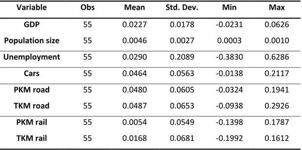
www.scb.se. Table 3 summarizes the descriptive statistics of GDP and traffic growth

seen over the entire sample period 1950-2005. The mean growth rate is considerably higher for traffic demand growth in terms of registered cars than for GDP growth (4.6 % versus 2.3 %) and considerably more volatile in terms of standard deviations (5.6% versus 1.8 %). The time series of unemployment rates in Sweden was retrieved via ECOWIN for the time period 1970-2005 and extended backwards using an unpublished series. Unemployment is by far the most volatile variable, mainly due to the sudden and persistent rise in unemployment at the beginning of the 1990s. The most stable variable is population size, thus ensuring that the per capita growth rates are close to the growth rates shown in Table 3.

Table 3: Descriptive statistics

Variable Obs Mean Std. Dev. Min Max

GDP 55 0.0227 0.0178 -0.0231 0.0626 Population size 55 0.0046 0.0027 0.0003 0.0010 Unemployment 55 0.0290 0.2089 -0.3830 0.6286 Cars 55 0.0464 0.0563 -0.0138 0.2117 PKM road 55 0.0480 0.0605 -0.0324 0.1941 TKM road 55 0.0487 0.0653 -0.0938 0.2926 PKM rail 55 0.0054 0.0549 -0.1398 0.1787 TKM rail 55 0.0168 0.0681 -0.1992 0.1612

Moreover, our analysis uses annual person-kilometer and ton-kilometer data for roads and railroads for the period 1950-2005. Ton-kilometer (TKM) and person-kilometer

Institute for Transport and Communications Analysis web-page. The methods used for constructing these time series are described in SIKA (2004). We can see that traffic growth in terms of both passenger kilometers and transport kilometers is circa 4.8 % per annum with a mean deviation of 6 %. In contrast, rail traffic grows considerably less, by about 0.5 % per year in terms of passenger kilometers and 1.7 % in terms of ton kilometers. The standard deviation in the time series of rail traffic is comparable to that of road traffic (5.5 % for passenger kilometers and 6.8 percent for ton kilometers). Figure 1 and Figure 2 visually compare GDP and the traffic demand measures used.

Figure 1: Comparison PKM (billion km) and GDP

5 0 0 0 0 0 1 0 0 0 0 0 0 1 5 0 0 0 0 0 2 0 0 0 0 0 0 G D P 0 2 0 4 0 6 0 8 0 1 0 0 1940 1960 1980 2000 Year... PKMroad PKMrail GDP

Figure 2: Comparison TKM (billion km) and GDP 5 0 0 0 0 0 1 0 0 0 0 0 0 1 5 0 0 0 0 0 2 0 0 0 0 0 0 G D P 0 1 0 2 0 3 0 4 0 1940 1960 1980 2000 Year... TKMroad TKMrail GDP

It is widely acknowledged that traffic demand and economic growth are strongly correlated. Moreover, evidence from Krüger (2009) shows that deviations from trend growth over different time scales (short term shocks and business cycles) reinforce this relationship for some types of traffic demand. Hence, traffic demand is likely to share important stochastic properties with GDP-growth.

Up to now, most have of the research on stochastic properties has focused on short.run traffic flow dynamics. Musha and Higuchi (1976) found evidence that short-run road traffic fluctuations are non-Gaussian and better modelled as a long memory process and a vast amount of later research has confirmed this finding. However, the question is whether such stochastic anomalies using high frequency data for relatively short time spans are adequate to model traffic demand for road projects with an economic life span of at least 40 years. Moreover, it is difficult to filter out the complex

patterns of seasonality exhibited by high frequency data. We therefore use a different approach and perform tests of long-range dependence on annual data described above covering longer time periods.

As a test for long memory we use a test based on Geweke and Porter-Hudak (1983). If a series exhibits long memory, it is an I(d) process, where d is a real number. For a stationary process d equals zero, and for a non-stationary process d equals one. The process is called fractionally integrated if d is not an integer value. The method uses nonparametric methods to evaluate d without explicit specification of the short-memory ARMA-parameters of the series. We also calculate the Hurst-parameter H as a measure of (anti-)persistence as follows (Percival and Walden 2000):

[

]

The results are summarized in Table 4.

Table 4: Results of fractional integration estimation

Data D H

GDP 1923-2005 0.28 0.78

Cars 1923-2005 0.13 0.63

TKM 1950-2005 0.20 0.70

PKM 1950-2005 0.58 Not defined

All the time series exhibited evidence of d>0 in growth rates and hence they are non-Gaussian. Gaussian noise is the basis for geometric Brownian motion (GBM) so that the results suggest that the use of GBM is inappropriate. GBM is widely used in finance, since it has the so-called martingale property. The martingale property simply states that changes in a process are independent from each other. Independent changes makes the future unpredictable which explains the use of GBM in finance since the notion of

unpredictability is consistent with the efficient market hypothesis and no arbitrage condition. For traffic demand there are no analogous reasons for rejecting long term persistence which would imply some degree of predictability. On the contrary, we would expect habits and switching costs creating persistence in traffic demand. For example, once we choose to buy a car or buy a house at a certain location, it is costly to switch to another mode of transportation. The long-memory property of traffic-demand we find for long-term aggregate data is confirming the short-run findings in earlier research. In the next section we proceed to examine the implications for real option valuations taking a road expansion as example.

4 Stochastic properties of traffic demand and real options: A

case study concerning road expansion

4.1 Assumptions

In order to reduce computational effort, we model the road expansion option as a so-called European option; that is, the option can only be exercised in a pre-specified future year. We assume that about 12,000 cars per month will use the 30-kilometre long road connecting A and B in either direction. Further, we assume that the trend growth in traffic flows is about 3 percent each year and that the traffic flows have a standard deviation of 5 percent per year. Based on these assumptions, we have to take the decision whether to invest immediately and, if we invest, how many additional lanes to build. The problem here is the comparison between a two-lane road soon becoming a bottleneck and a four-lane road plagued by higher costs and underused capacity. The cost per lane is 1 million Euro.

The benefits from new roads are mainly time savings and increased safety. The time savings are zero if congestion is sufficiently large. We assume here that the comparison alternative would imply an average speed of 70 km/h. That is, the journey between A and B will take 25.7 minutes. The highway, however, allows for an average speed of 90 km/h, so that the 30-kilometer long journey only takes 20 minutes. If we assume that the average value-of-time is 10.5 Euro per hour, this corresponds to 1 Euro per car. We assume, therefore, that each car using the road up to the capacity limit is valued at 1 Euro.

We further assume, in line with other research, that a road can absorb a significant amount of traffic above capacity limits, but that the benefits for society of this extra traffic are zero. For each car entering above the capacity limit we can think of

congestion costs that reduces the overall net benefits. For example, if the net benefits for the driver entering the road is 1 Euro on average (assuming the alternative route represents a value of .99 Euro), if the (external) congestion costs is 0.01 Euro per car and 100 cars simultaneously using the affected road section, this implies that the individual benefit is 1 Euro (otherwise the driver would not use the road), but that the sum of marginal disutility for all others is 1 Euro as well and hence we have that societal net benefits is reduced to 0 Euro. Since the uncertainty with regard to traffic demand on a certain road is more pronounced than uncertainty with regard to maintenance costs, and that maintenance costs can be sufficiently determined by deterministic models as a function of road usage, we assume that costs per car are constant in real terms. The cost of preparation of a two-lane road with a later expansion option is hard to estimate correctly. Ex-ante we do not specify any construction cost for the road expansion. Ex-post, we can interpret the value of flexibility as the upper boundary for the cost road expansion.

We proceed as follows. First, we present a simple standard simulation model based on geometric Brownian motion in order to quantify the option value of road expansion. Second, based on the results of time series analysis and previous research on traffic demand, we estimate the impact of alternative stochastic processes on option value.

4.2 Standard model based on geometric Brownian motion

The investment decision is dependent on future demand. It is hard to predict the exact number of cars since this depends on many different factors. However, looking at the materialized traffic demand as one realization of a stochastic process followed by traffic demand, we can draw interferences with regard to the underlying process. Based on

that, we can simulate future traffic flows. Each sample path represents a different history. Each of these proposed future traffic paths are extremely unlikely to be correct, but we can construct a distribution of traffic demand for each future point in time. Using these distributions we calculate expected values and take decisions (given risk neutrality). The starting point for our analysis is the Geometric Brownian motion often used in real option valutation:

TVdB TVdt

dTV =µ +σ (4)

Where TV is the monthly traffic volume and µ is the drift rate, σ is the volatility measured as standard deviations and dB is the infinitesimal increment in a Brownian motion. In order to simulate the sample paths we make use of the explicit solution to the geometric Brownian motion (Oksendahl 2000):

t B t t TV e

TV = ₀ (µ−0.5σ2)+σ (5)

It is obvious that the road value is dependent on the realized path. Even a small volatility has a major impact on the range of possible future outcomes. The assumption of a geometric Brownian motion means that traffic is normally distributed, which in turn implies that future traffic is log-normally distributed.

The alternative with 2 lanes only is restricted to 15,000 cars per month. Another feasible alternative is to immediately invest in a four-lane road (with capacity 30,000 cars per month), thus providing more capacity in case road traffic grows fast in the years to come. However, on investing immediately in 4 lanes we have unused capacity in many cases over a long period; in the most optimistic case we will reach capacity limit in 15 years, but in many cases we will never have to use the additional capacity. Hence, an alternative is to wait and eventually invest later in an expansion to 4 lanes. Figure 3 illustrates the real option case.

The results from the Monte-Carlo simulation based on the geometric Brownian motion are given in Table 5 and illustrated in Figure 3. According to these results we will prefer the 2-lane road to the 4-lane road. Thus, the cost of a too low capacity caused by foregone benefits is less than the capital costs of underutilized capacity. The flexible alternative would be to build 2 lanes now and later expand to 4 lanes (see Figure 4). As outlined above, that would require certain measures like the purchase of right of way and the adaptations of bridges and tunnels, so that the expansion may take place in the future when we have more information with regard to traffic demand. According to Table 5 the real option alternative is preferable compared to the other alternatives if the additional costs are not larger than 240 thousand Euro.

Figure 3: Simulation of traffic demand

0 5 10 15 20 25 30 35 40 1 2 3 4 5 6 7 8 9 10x 10 4 t TV(t)

Table 5: Present value of 2 lanes, 4 lanes and real option alternative

Alternative Present value

2 lanes 1.959 600 Euro

4 lanes 1.816 800 Euro

Figure 4: Payoff from real option alternative 0 5 10 15 20 25 30 35 40 1 1.2 1.4 1.6 1.8 2 2.2 2.4 2.6 2.8 3x 10 4

The reason for this result is that we do not have to finance unused capacity in the first years. The real option value can be divided into two parts: the pure value of waiting and the value of information. The first effect is the result of the fact that the benefits (traffic demand) grow more slowly than the discount rate. Hence, the benefits are discounted less than the costs, so that it is optimal to postpone investments. The second effect is the result of information with regard to the status of the stochastic process; that is, we only expand the road when sufficient traffic demand growth has materialized. In the cases of traffic demand being low, we will probably never have to use the expansion option. If we do not sort out the outcomes with low future traffic demand, the flexible alternative becomes less valuable. The difference is approximately 56.2 thousand Euro (see Table 5). Hence, we get a higher value if the option is exercised only in the 66 percent of total paths where the outcome lies above 15,000 cars in 10 years. The optimal threshold can, in principle, be determined by Equation 2. We use a numerical approach to determine the threshold value maximizing option value.

4.3 Alternative model based on fractional Brownian motion

Since we have provided some empirical evidence that traffic demand might be better characterized by stochastic processes other than the normal distribution, we check whether the assumption that noise around trend growth is Gaussian (H=0.5) is crucial for real option valuation. As an alternative we model the process as follows:

TVdF TVdt

dTV =µ +σ

with dF = f

(

σ

)

(6)

This can be written as:

dF dt TV dTV σ µ + = (7)

where dF is the increment of fractional Brownian motion with parameters σ measuring volatility and H measuring (anti-)persistence. Hence, the percentage increase in traffic demand is expected to grow with µ and uncertainty (that is, the confidence interval around the expectation) about future traffic growth rates increases by tH per year. Hence, the future traffic volume is distributed as follows:

(

µ

σ

)

Thus, for persistent processes with H>0.5 the range of possible outcomes grows faster than the square root of time predicted by the geometric Brownian motion.

The parameter H can take values between zero and one. We simulate 100,000 sample paths for each value of H between 0.1 and 0.9 with step size 0.1, and use the Euler approximation scheme (Mikosch 1998) to numerically solve the stochastic differential equation driven by fractionally integrated noise proposed in Equation 6. Solving a stochastic differential equation means that we can compute the value of the process given the status of the underlying stochastic process. The Euler-approximation scheme can be described by the following set of equations:

0 0 TV TV = (9) n T t = ∆ (10) t i t i t F F F i = ∆ − − ∆ ∆ _{( 1)} (11) n i F TV t TV TV TV i t t i t i t i t i∆ = (−1)∆ +µ (−1)∆∆ +σ (−1)∆ ∆ ∀ =1,..., (12)

Figure 5 illustrates and compares the explicit solution of the GBM with the solution provided by the Euler approximation scheme using 5, 20 and 100 steps. Obviously, the quality of the approximation scheme depends on the number of simulated steps.

Figure 5: Numerical solution with 5, 20, 100 steps & explicit solution of GBM

Because of the flexibility provided by the Euler approximation, we use it to solve Equation 6 numerically. An analytic solution to the FBM exists, but the Euler scheme allows for a simpler adaption to alternative formulations of the underlying process for traffic. It is in principle possible to combine FBM with mean reversion, jump processes or additive noise. Such and similar extensions might be interesting alternatives to the formulation of FBM with trend used here. The simulated sample paths are used to evaluate the option value defined as the difference between the flexible solution and best inflexible solution (either two lanes or four lanes). The estimated option value

indicates the amount that can be spent today to increase future flexibility with regard to traffic demand. Table 6 and Figure 6 show the results.

Table 6: Option value in thousand Euro, H and threshold level

Figure 6: Option value as a function of H and the threshold

0.1 0.2 0.3 0.4 0.5 0.6 0.7 0.8 0.9 12000 13000 14000 15000 160000.5 1 1.5 2 2.5 3 3.5 x 106 H Threshold Option Value H 0.1 0.2 0.3 0.4 0.5 0.6 0.7 0.8 0.9 Threshold 12,000 158.2 156.3 156.7 153.0 157.4 170.1 192.5 226.4 272.5 13,000 157.7 159.0 159.8 163.3 170.9 188.1 219.9 258.2 308.2 14,000 157.7 159.1 163.2 170.4 182.8 206.2 235.5 275.6 324.9 15,000 136.0 140.8 150.4 163.2 182.2 206.6 240.2 282.5 335.2 16,000 72.7 81.0 89.0 130.4 158.8 192.5 228.8 273.5 330.3

We see that the option value varies with the value of H of the stochastic process. Anti-persistent behaviour lowers the option value, since traffic demand reverts to its long-run growth level. The degree of uncertainty and therefore the value of flexibility are therefore less compared to the case when H=0.5. When the cumulative noise process instead exhibits long memory (H>0.5), the value is higher, since unforeseen stochastic shocks generate long cycles that change the probability that traffic demand forecasts (the confidence interval around the expectation) grow faster than the square root of time predicted by geometric Brownian motion. Given that there is some evidence that we have long memory, it seems that the option value is higher than predicted by the standard model. In our example, the option value is 3% higher than predicted by the GBM for H=0.6 and 10% higher for H=0.7. Moreover, the non-linear impact of the persistence parameter H on the option value is a non-trivial insight gained from our analysis. Interestingly the optimal threshold level for exercising the expansion option depends positively on the Hurst-parameter, so that the optimal threshold is higher for persistent processes than for Gaussian processes. This indicates that the information value of observed traffic flows is higher for persistent processes.

5 Concluding remarks

The purpose of the paper was i) to examine the time series property of traffic demand and ii) to analyze the impact of stochastic properties on real option valuation. As a case study the paper analyzes the real option value that can be obtained by adapting certain critical construction elements and right of way purchase so that a later road expansion from two to for four lanes is possible at a lower cost. Based on the statistical analysis of GDP and traffic demand, we conclude that traffic demand evolution is characterized by persistence. An economic shock boosting traffic demand growth will result in higher

future traffic demand growth, for example by establishing new habits. This has important implications on real option valuation since the degree of future uncertainty is higher than predicted by the standard model. We therefore advocate further research on the time series properties of traffic demand, since it is a central issue when planning huge irreversible road investments. The use of the risk-neutral interest rate used in many real-option applications of infrastructure can be questioned based on the time series properties we found. Furthermore, even if the standard model might be convenient to derive comparative-statics in conceptual real-option models related to transportation, we think that in real-life applications planners should acknowledge our empirical findings.

References

Andersson, H. (2003). “Valuation and hedging of long-term asset-linked contracts.” Economic Research Institute, Stockholm School of Economics (EFI): Stockholm. Dixit, A. K. and Pindyck, R. S. (1994). “Investment under Uncertainty.”, Princeton University Press.

Flyvbjerg, B., Bruzelius, N. and Rothengatter, W. (2003). “Megaprojects and Risk: An anatomy of ambition.” Cambridge University Press.

Krüger, N. (2009), “Infrastructure Investment Planning under Uncertainty”, PhD-Dissertation, Örebro Studies in Economics #17.

McDonald, R. and Siegel, D. (1986). “The Value of Waiting to Invest.” The Quarterly

Journal of Economics, 101(4), 707–728.

Mikosch, T. (1998). “Elementary Stochastic Calculus.” Advanced Series on Statistical Science & Applied Probability, World Scientific.

Musha, T. and Higuchi, H. (1976). “The 1/f fluctuation of a traffic current on an expressway.” Japanese Journal of Applied Physics, 15(7), 1271-1275.

Oksendahl, B. (2000). “Stochastic Differential Equations- An Introduction with Applications.” 5th ed., Springer-Verlag: Heidelberg and New York.

Olsson, K. O. (2003). “New Evaluation Methods for Rail and Road Investments – An Approach based on Real Options.” School of Economics and Commercial Law, Göteborg University, Göteborg.

Saphores, J.-D and Boarnet, M.G. (2006). “Uncertainty and the timing of an urban congestion relief investment - The no-land case.” Journal of Urban Economics, 59(2), 189-208.

Smit, H. (2003). “Infrastructure Investment as a Real Options Game: The Case of European Airport Expansion.” Financial Management 32(4), 27–57.

Percival P. D. and Walden T. A. (2000). “Wavelet Methods for Times Series Analysis.” Cambridge University Press.

Zhao, T. and Fu, C. C. (2006). “Infrastructure Development and Expansion under Uncertainty: A Risk-Preference-Based Lattice Approach.” Journal of Construction

Engineering and Management, 132(6), 620-625.

Zhao, T. and Tseng C.-L. (2003). “Valuing Flexibility in Infrastructure Expansion.”

Journal of Infrastructure Systems, 9, 89-97.

Zhao, T., Sunderarajan, S. K., and Tseng C.-L. (2004). “Highway Development Decision-Making under Uncertainty: A Real Options Approach.” Journal of

Infrastructure Systems, 10, 23-32.

MATLAB-code for simulation study:

% This program evaluates alternatives based on the simulation of fractional % Brownian noise clear; for hi=1:9; for tl=1:5; clear t; S_0=12000; T=39; mu=0.03; sigma=0.05; dt=1; N=500; Steps=T/dt; t(1,:)=1:40; t=repmat(t,N,1);

H=hi/10; % Hurst-index between 0.1 and 0.9 if H==0.5; H=0.5+0.000000001; % ffgn needs H<0.5 or H>0.5 end; FN=ffgn(sigma,H,N,40,0); W_tl= cumsum(FN,2); W_t=transpose(W_tl); S(1,1:N)=12000; for i=2:40; for j=1:N; S(i,j)=S(i-1,j)+1*S(i-1,j)*(W_t(i,j)-W_t(i-1,j))+S(i-1,j)*mu; end; end; % figure(1)

% plot([0:dt:T],S); % plot S_t against t

%xlabel('t','FontSize',16);ylabel('TV(t)','FontSize',16,'Ro tation',0); %Alt1:2way A=min(S,15000); %figure(2)

%plot([0:dt:T],A); % plot S_t against t

%Alt2:4way

B=min(S,30000); %figure(3)

%plot([0:dt:T],B); % plot S_t against t

%Alt3:2way+ev 4way in 10 years C=A(1:40,1:N); B2=B; A2=A; for i=1:N;

if S(10,i)>10999+tl*1000; %Threshold between 12000 and 16000 C(11:40,i)=B2(11:40,i); y(i,1)=1; else C(11:40,i)=A2(11:40,i); y(i,1)=0; end end %figure(4)

%plot([0:dt:T],C); % plot S_t against t %CBA of alternatives %Alt1 for i=1:40; for j=1:N; CA(i,j)=A(i,j)*10*12*exp(-0.05*t(1,i)); end; end; DCA=sum(CA,1); EDCA=sum(DCA,2)/N-10000000; %Alt2 for i=1:40; for j=1:N; CB(i,j)=B(i,j)*10*12*exp(-0.05*t(1,i)); end; end; DCB=sum(CB,1); EDCB=sum(DCB,2)/N-20000000; %Alt3 for i=1:40; for j=1:N; CC(i,j)=C(i,j)*10*12*exp(-0.05*t(1,i)); end; end; DCC=sum(CC,1);

EDCC=max(sum(DCC,2)/N-10000000-p*10000000*exp(-0.05*10));

OV(tl,hi)=EDCC-max(EDCA,EDCB);%Option values for different H and Thresholds end; end; % Create figure figure1 = figure('PaperSize',[20.98 29.68]); colormap('gray'); % Create axes axes1 = axes('Parent',figure1,... 'YTickLabel',{'12000','13000','14000','15000','16000','3.5' ,'4','4.5','5'},... 'YTick',[1 2 3 4 5],... 'XTickLabel',{'0.1','0.2','0.3','0.4','0.5','0.6','0.7','0. 8','0.9'},... 'XTick',[1 2 3 4 5 6 7 8 9],... 'Position',[0.13 0.11 0.775 0.815],... 'FontSize',16,... 'CLim',[0 1]); xlim([1 9]); ylim([1 5]); view([-45.5 20]); grid('on'); hold('all'); % Create surf surfl(OV); % Create xlabel xlabel({'H'},'FontSize',20); % Create ylabel ylabel('Threshold','FontSize',20); % Create zlabel zlabel({'Option Value'},'FontSize',20);