3(4): 587-611, 2013 SCIENCEDOMAIN international
www.sciencedomain.org
An A-Train Satellite Based Stratiform
Mixed-Phase Cloud Retrieval Algorithm by Combining
Active and Passive Sensor Measurements
Loknath Adhikari
1and Zhien Wang
1*1University of Wyoming, Laramie, WY, USA. Authors’ contributions This work was carried out in collaboration by both authors. Author ZW designed the study. Author LA carried out the analysis and wrote the first draft of the manuscript. Both authors were involved in managing the manuscript.
Received 2ndNovember 2013 Accepted 2ndNovember 2013 Published 18thNovember 2013
ABSTRACT
Aims: To develop a new satellite-based mixed-phase cloud retrieval algorithm for
improving mixed-phase cloud liquid water path (LWP) retrievals by combining Moderate Resolution Imaging Spectroradiometer (MODIS), CloudSat, and Cloud-Aerosol Lidar and Infrared Pathfinder Satellite Observations (CALIPSO) measurements.
Study Design: Algorithm development and evaluation by using collocated NASA A-Train
and the Atmospheric Radiation Measurement (ARM) Climate Research Facility (ACRF) measurements at the North Slope Alaska (NSA) site.
Place and Duration of Study: Collocated MODIS and ground-based measurements at
NSA site from March 2000 to October 2004, MODIS measurements and retrievals during July 2006 over Eastern Pacific, and MODIS, CloudSat and CALIPSO measurements on April 04, 2007 over the Arctic Region.
Methodology: The stratiform mixed-phase cloudswere treated as two adjunct water and
ice layers for radiative calculations with the Discrete Ordinate Radiative Transfer (DISORT) model. The ice-phase properties were provided with the 2C-ICE product, which is produced from CloudSat radar and CALIPSO lidar measurements, and they were used as inputs in DISORT for the calculations. Then, the calculated mixed-phase cloud reflectances at selected wavelengths were compared with MODIS reflectances to retrieve liquid-phase cloud properties.
clouds by using MODIS radiances and ice cloud properties from active sensor measurements. The algorithm was validated separately by using Operational MODIS retrievals of warm marine stratiform clouds and collocated surface measurements of Arctic stratiform mixed-phase clouds. The results show that the new algorithm reduced the positive LWP biases in the Operational MODIS LWP retrievals for stratiform mixed-phase clouds from 35 and 68% to 10 and 22% in the temperature ranges of -5 to -10ºC and -10 to -20ºC, respectively.
Conclusion: The combined A-Train active and MODIS measurements can be used to
improve global mixed-phase cloud property retrievals.
Keywords: Stratiform mixed-phase clouds; CloudSat;, CALIPSO; MODIS; the A-Train satellites; retrieval algorithm.
ACRONYMS
ACRF: Arm Climate Research Facility; AERI: Atmospheric Emitted Radiance Interferometer; ARM: Atmospheric Radiation Measurement; BT: Brightness Temperature; CALIOP: Cloud-Aerosol Lidar with Orthogonal Polarization; CALIPSO: Cloud-Cloud-Aerosol Lidar and Infrared Pathfinder Satellite Observations; CPR: Cloud Profiling Radar; CTT: Cloud Top Temperature; CWC: Cloud Water Content; DISORT: Discrete Ordinate Radiative Transfer; GCM: General Circulation Model; IWP: Ice Water Path; LWP: Liquid Water Path; MMCR:: Millimeter Wavelength Cloud Radar; MODIS: Moderate Resolution Imaging Spectroradiometer; MPL: MicropulseLidar; MWR: Microwave Radiometer; NASA: National Aeronautics and Space Administration; NSA: North Slope Alaska; POC: Pockets of Open Cells; SHEBA: Surface Heat Budget of the Arctic Ocean; TOA: Top Of the Atmosphere; UV: Ultra Violet; VAMOS: Variability of the American Monsoon Systems; VOCALS-Rex: VAMOS Ocean-Cloud-Atmosphere-Land Study Regional Experiment.
1. INTRODUCTION
Clouds are important because of their roles in the global hydrological cycle and transport of heat and moisture from low latitudes towards the poles [1,2]. Besides, they are important regulators of the earth’s radiation balance [3-5]. It is also well known that the impact of clouds strongly depend on cloud phases and properties [6-8]. Clouds exist as water droplets at temperatures > 0ºC and ice crystals at temperatures < -40ºC, but between 0ºC and -40ºC both water and ice phases can coexist [9-13].
Mixed-phase clouds are particularly important in the Polar Regions, where they are the most dominant clouds and strongly influence the surface radiation balance. [14,15] reported that mixed-phase clouds occur 41% during Surface Heat Budget of the Arctic Ocean (SHEBA) and are more frequent during the spring and fall transition seasons. Aircraft observations in Beaufort and Arctic Storm Experiment (BASE) showed that 90% of the sampled boundary layer clouds (during September – October) were mixed-phase clouds. Furthermore, [16] showed that middle-level stratiform phase cover is over 5% globally. These mixed-phase clouds have significant radiative impacts at the top of the atmosphere (TOA) and the surface [17].However, the properties and evolutions of these mixed-phase clouds are difficult to simulate [18,19]. The simulations of these clouds in general circulation models (GCM) are the main sources of cloud uncertainties in the polar regions [20,21]. The radiative properties of the mixed-phase clouds depend on the relative amounts of liquid and ice phases, which
are controlled by complicated cloud microphysical processes. Therefore, it is urgent to better observe and understand mixed-phase cloud properties.
Ground-based combined active and passive remote sensing measurements have been successfully applied to retrieve ice and water phases separately in mixed-phase clouds [14, 15,22,23]. For example, [22] treated the stratiform mixed-phase clouds as supercooled liquid-dominated mixed-phase layer with ice virga falling out of its base. Then they used combined lidar and radar measurements to retrieve properties of the ice virga and combined the retrieved ice properties with radiance measurements from atmospheric emitted radiance interferometer (AERI) to retrieve liquid cloud properties. Although, these ground-based algorithms provide valuable mixed-phase cloud properties, the long-term multi-sensor ground-based measurements are limited to a few locations. In considering highly variable mixed-phase cloud properties due to dynamics and aerosol variations, it is important to have global mixed-phase cloud properties for model evolutions and process-oriented studies. However, the progress of research in retrieving mixed-phase cloud properties from satellite measurements is slow. Widely used MODIS retrieved cloud properties, effective radius (re),
optical depth () and liquid/ice liquid water path (LWP/IWP), are only applied to single-phase clouds [24-26]. Most stratiform mixed-phase clouds are treated as liquid clouds in the Operational MODIS products resulting biased LWP retrievals. There are great efforts being made to improve MODIS mixed-phase cloud retrievals [27]. [28] Demonstrated that adding additional measurements at visible wavelengths could provide ice and liquid properties for mixed-phase clouds. However, retrieving mixed-phase cloud properties with passive measurements is still a challenging task. Current CloudSat cloud water content (CWC) product provides both liquid and ice water retrievals based on a simple temperature dependent mass partition due to limited information from radar-only measurements [29,30]. Nonetheless, the simultaneous collocated active and passive remote sensing measurements from NASA A-Train satellites offer new opportunities to provide mixed-phase cloud properties.
Here, we present a new approach to retrieve stratiform mixed-phase cloud properties by using MODIS radiance measurements and CloudSat and CALIPSO measurements. The general principle is to use CloudSat and CALIPSO measurements to provide ice phase properties [31] and to use MODIS to provide liquid phase properties. Although MODIS is a cross-track scanning radiometer, while CloudSat and CALIPSO measure along the orbital track, MODIS footprints can be collocated along the CloudSat track for the A-Train based retrieval. The new mixed-phase algorithm is developed and tested in multi-steps. First, the algorithm is compared with the MODIS retrievals for warm marine stratiform clouds in the Eastern Pacific (20 – 30ºN and 120 – 140ºW) to assess the performance of the new retrieval algorithm for ideal, homogeneous warm water-only clouds. Then, we use collocated long-term MODIS and ground-based measurements at the Atmospheric Radiation Measurements (ARM) Climate Research Facility (ACRF)North Slope Alaska (NSA) site to evaluate the new MODIS based LWP retrievals for mixed-phase clouds with ice properties (IWP and Dge) from
surface multi-sensor measurements as inputs due to of the lack of sufficient coincident CloudSat and CALIPSO measurements over the NSA site. Finally, we apply the algorithm to the A-train measurements by combining MDOIS radiance with ice properties from the 2C-ICE product. This paper is organized in the following way. Section 2 provides a description of the algorithm followed by error analysis in section 3. Section 4 provides the validation of the mixed-phase algorithm for warm marine stratiform clouds and Arctic mixed-phase clouds. Then, section 5 provides a case study to illustrate the use of the algorithm for A-Train
2. ALGORITHM DESCRIPTION
2.1 The General Setup of the Algorithm
The algorithm is intended for simultaneously retrieving the effective radius (re, based on) [32]
and optical depth () for low and mid-level stratiform mixed phase clouds. We used reflected solar radiance measurements from 1.24 and 2.13m MODIS bands with ice properties from active sensor measurements to retrieve re and . Thus the mixed-phase retrieval algorithm
inherits the general characteristics of the operational MODIS retrieval method [33] with modifications to allow for the presence of both liquid and ice phases in the clouds for radiative calculations.
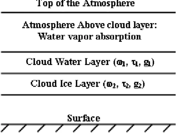
The structure of the modeled cloud and atmosphere for the retrieval is shown in Fig. 1. The main assumptions used in setting up the radiative transfer calculations are as follows:
1. The atmosphere is plane parallel.
2. Rayleigh scattering by molecules is negligible and can be ignored in the radiative transfer calculations at wavelengths longer than 1m.
3. The mixed-phase clouds are treated as two adjacent liquid and ice layers.
As shown in the figure, the top most layer of the modeled atmosphere represents the absorption of radiation by water vapor present above the cloud. The Rayleigh scattering by atmospheric molecules is very small for the wavelengths used in the retrieval algorithm, so the Rayleigh scattering effects can be ignored in the radiative transfer calculations [26,33]. The surface albedo used in the radiative calculations is from the 16-day mean surface albedo values in the MODIS BRDF/albedo [34].
Fig. 1. The vertical structure of the cloud-atmosphere system used for stratiform mixed-phase cloud retrievals
Ground-based lidar and radar measurements at the NSA site have demonstrated that the stratiform mixed-phase clouds have a simple vertical structure: a thin super cooled water dominated mixed-phase layer at the top with a deep ice virga layer below, although multiple super cooled water layers in the mixed-phase clouds do occur [15,17,22]. Surface multi-sensor observations at the NSA site showed that liquid phase counts for over 75% of the
total mass in the super cooled water dominated mixed-phase layer [19]. This feature is also confirmed with in-situ data [15,35,36]. Considering the significantly larger liquid fraction and smaller water droplet size compared to ice crystals, it is clear that the number concentration of water droplet is significantly larger than that of ice crystals. As a result, liquid phase dominates the optical depth of this thin mixed-phase layer. Therefore, treating the stratiform mixed-phase clouds with two separate liquid and ice layers is a validapproximation for radiative transfer calculations, although it does not fully describe the details of the mixed-phase clouds. These stratiform clouds with liquid dominated mixed-mixed-phase layer with ice virga below is commonly observed over the polar regions; however, study by Zhang, et al. [16] showed that they are observed globally and have profound impact on the radiative balance of the earth.
2.2 The Forward Model
In the retrieval of cloud and re, the Discrete Ordinate Radiative Transfer (DISORT) model
was used to compute the reflected radiance [37,38]. DISORT solves the transfer of monochromatic radiation in a scattering, absorbing, and emitting plane-parallel medium [37]. Its versatility allows DISORT to be used for atmospheric processes ranging from ultraviolet (UV) to the microwave regions.
The reflected radiance (Iλ(0,-μ,ϕ)) when normalized with the incident solar flux (F
0) gives the
reflection function Rλ(
i,re,μ,μ0,ϕ) as [24]:
( , ; , , ) =
( , , )( )
… … … …
(1)where,iis the cloud optical thickness, μ, μ0andare the cosine of the satellite zenith angle
(), cosine of the solar zenith angle (θ0), and the relative azimuth angle between the
direction of propagation of the emerging radiation and the incident solar radiation, respectively.
For a given geometry between the sun and the satellite, Rλ(
i,re;μ,μ0,ϕ)is a function ofiand
rewhich are the total contribution of liquid and ice. The key of the forward model is to provide
optical properties as required for DISORT calculations. The general procedure of the forward model is shown in Fig. 2.
The critical step in setting up the DISORT model is to provide single scattering albedo (i),i
and asymmetry parameter (gi) for both liquid and ice layers. The single scattering properties
of poly-disperse distributions of cloud droplets are largely insensitive to the actual shape of the size distribution, but depend mostly on re[39]. We used lognormal size distribution with
effective variance of 0.11 to model the size distribution of the cloud droplets. TheIand giof
cloud droplets were calculated as a function of re by using the Mie theory. The complex
refractive indices of water required for the calculations were obtained from [40] for the 1.24 µm band and [41] for the 2.13 µm band.
Fig. 2. Flowchart showing the structure of the forward model for calculating the look up table
The i and gi for ice crystals are strongly dependent on ice crystal size and shape [42]. Ice
crystal shapes are also strong functions of temperature and growing history [43-45]. Many parameterizations were developed to simplify the calculations of and g for ice crystals. For example, MODIS uses the mixture of several common ice crystal shapes as its ice model for pure ice cloud retrievals [33]. Considering the differences of ice crystal shapes in the mixed phase clouds compared to cold pure ice clouds, we use the parameterization scheme developed by Fu [46] to determinei and gi as a function of general effective size (Dge),
which is given by:
= √ ( ) … … … …. (2) Similarly, the parameterization of Fu [46] is also used to derive the ice optical depth with ice water content and Dgeas shown in eq. 3.
= ( + … … … . … … … .. (3)
2.3 A Calculation Example of Lookup Table
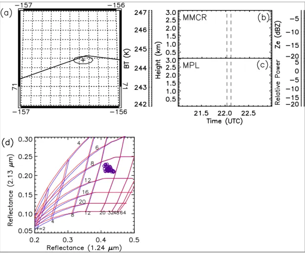
For fast retrievals, we use the forward model to develop lookup tables as the Operational MODIS algorithm. A lookup table is calculated for given ice cloud properties represented by IWP, (Dge) and g(Dge), the zenith and azimuth angles of the sun (0,0), and the satellite
(,), along with 32 values of re ranging from 3.13 to 36.41 µm (Appendix A) and values of
ranging from 0 to 100 at an interval of 0.1. Fig. 3 shows an example of lookup table used in the retrieval process. Fig. 3(a), which shows MODIS 11.03 m brightness temperature, shows uniform BT (~244 K) around the NSA site. The MMCR Ze (Fig 3(b)) and MPL power (Fig. 3(c)) show low level clouds with cloud tops at ~ 1.1 km. The MPL backscatter power also shows liquid-dominated layer at the top (the region with high backscatter power). Fig. 3(d) shows different responses of reflection functions at 1.24 m (band) 5 and 2.13 m (band 7) wavelength pair. The horizontal and vertical lines represent reflection functions at
specified values of re and specified values of , respectively. Reflectances were calculated
for two different scenarios: (1) water-only clouds in red and (2) mixed-phase clouds in blue. The overlaid circles in the figure are measurements of reflectances from MODIS on 2205Z, June 02, 2000 around a 3-pixel radius centered at the NSA site. The cloud vertical structure and ice layer properties are provided based on ARCF ground-based measurements: mixed-phase clouds with the top at 1.2 km, base of the water layer at 0.9 km, with IWP and Dgeof
9.9 g/m2and 81.8µm, respectively.
Fig. 3. (a) MODIS 11.03 m brightness temperature map around the NSA site. The NSA site is shown by (+) and the position of the 33 MODIS footprints around the NSA site
are shown by the oval. (b) MMCR Ze, (c) MPL backscatter power. The vertical dashed lines represent the 5-minute period centered at the satellite overpass time.(d) The different responses of the reflectances of 1.24 and 2.13 m bands as a function of liquid-phase reand for water-only clouds (red curves) and mixed-phase clouds (blue
curves) with precipitating ice virga (Dge=81.8m, IWP=9.9 g/m2), respectively. The
overlaid circles are the MODIS measurements from on 2205Z, June 02, 2000 around a 3-pixel radius centered at the NSA site. The example is for = 29.7°, 0= 49.1° and =
68.3° with surface albedo of 0.30 and 0.10 for 1.24 and 2.13 µm MODIS bands, respectively.
The figure clearly highlights the principle of the retrieval method: the reflection function at 1.24 µm has a greater dependence on with a weaker dependence on re, whereas the
reflection function at 2.13 µm shows a greater dependence on re, with larger reflectances at
smaller reand small reflectance at larger re. Meanwhile, the figure shows the impacts of ice
phase on mixed-phase cloud reflectances. In general, the reflectance for mixed-phase clouds shifts to up and left. Therefore, with the same observed reflectance, the retrieved re
and are smaller for mixed-phase clouds than for liquid-only clouds. The difference is particularly large at low. As theof the cloud layer increases the calculated radiances from liquid-only and mixed-phase clouds converge, which shows that the contribution of the ice layer to the reflectance decreases with increasingof the liquid layer as expected.
2.4 Retrieve LWP and r
eThe simultaneous retrieval of reandwas done in a two-step method. (1) The look up table
of reflectance was created from the forward calculations ( , ) for given ice-phase properties and the MODIS measured reflectance ( ) to define a residual function given by:
= [ln . − ln . ( , )] + [ln . − ln . ( , )] … … … … ( 4)
The residual function is a function of reand, so a combination of reandcan be found that
minimized the residual function and is taken as the first approximation for reand. (4) The re
obtained from step (1) was then further refined to obtain the best estimation of re due to
coarse resolution of rein the look-up table. For a known value of , the reflectances become
functions of realone, given by:
− ( ) = 0. … … … (5) Eq. 5 can be approximated by polynomial equations in reof the form:
+ + + = 0 … … … . .. (6) Where, A0, A1, A2and A3are coefficients determined from the lookup table. Solution of Eq. 6
gives the best estimate re. Since the look up table containedvalues at an interval of 0.1, no
further refinement was applied to in the second step. The value of obtained in the first step and the value of reobtained in the second step were used to calculate the LWP [47].
3. ERROR ANALYSIS
As shown in Fig. 2, the inputs to the radiative transfer calculations include the optical parameters of super-cooled liquid water droplets, the geometry of the sun and the satellite, the ice-phase Dge and IWP and the surface albedo. The sun and the satellite zenith and
azimuth angles are well calibrated in the MODIS data and the refractive indices of liquid water are well known .Similarly, uncertainties in water vapor absorption introduce uncertainties in reflectance from the forward model, but these uncertainties are less than < 1 %. Thus, the main sources of uncertainties in the forward model come from uncertainties in the ice cloud properties and the surface albedo.
3.1 Sensitivity to Surface Albedo
The measured reflectance has contributions from both the surface (through surface albedo) and the cloud. Hence, the choice of the surface albedo can have impacts on the retrieved LWPs as expected, especially for clouds with low optical depths. Fig. 4(a) and 4(b) show the absolute and relative sensitivities of calculated reflectances at 1.24 µm (blue) and 2.13 µm (red) bands to a 20% uncertainty in the surface albedo values as a function of cloud LWP. The true albedo values for 1.24 and 2.13 µm bands are 0.30 and 0.10, respectively, indicating surface covered by snow and sea ice. The figure shows that the reflectances are positively correlated with the surface albedo, so an over estimation in the surface albedo leads to an overestimation in the calculated reflectance, and vice versa. However, the two MODIS bands show different sensitivities to the changes in the surface albedo. The 1.24 µm band is more sensitive to the changes in the surface albedo than the 2.13 µm band because the former band is more sensitive to and the latter is more sensitive to re. For the 1.24 µm
band, the impacts decrease almost exponentially from ~ 18% at LWPs < 5 g/m2 to 5% at
LWPs 30 g/m2. However, for the 2.13 µm band, the change in the reflectance drops below
1% for LWPs > 30 g/m2. Fig. 4(c) shows the errors in retrieved LWP for the four possible combinations of 20% change in the surface albedo, viz. decrease in both bands (dashes), increase in both bands (long dashes), decrease (increase) in 1.24 (2.13) µm (dash-dot) and increase (decrease) in 1.24 (2.13) µm (dashes with multiple dots). The retrieved LWP is overestimated when the surface albedo is biased low and vice versa. The largest error in the retrieved LWP comes from the combination of surface albedosbiased in the opposite direction. The percentage errors in the retrieved LWP due to 20% error in the surface albedo decrease as LWP increases. For clouds with LWP of 20 g/m2, a 20% underestimate or overestimate of the surface albedo leads to a ~ 50% overestimate or underestimate in the retrieved LWP. However, for clouds with LWP greater than 50 g/m2, the retrieval error in
LWP is < 10%.Furthermore, we picked high surface albedo case for sensitivity study, and the errors are the upper-bounds and random errors due to albedo. Fig. 4(d) shows the change in retrieved LWP when different fraction of MODIS footprints contain open water surface (surface albedo of 0.061 and 0.040 for 1.24 and 2.13 m, respectively) instead of snow/sea ice surface, which could occur in the sea ice melting season briefly when 16-day mean albedo is used. The figure shows that the retrieved LWP is overestimated for ocean surface, and the positive bias decreases with decreasing fraction of open water surface. Although the positive bias in retrieved LWP is large for MODIS footprints that lie in the open water surfaces and incorrectly treated as ice/snow surface, the error for LWP > 20 g/m2
when averaging over a 9-pixel box around the NSA site is < 10%. Thus, in the following comparison study at the NSA site, surface albedo is not expected to introduce significant uncertainties in LWP retrievals.
Fig. 4. (a) Variation of reflectance of MODIS 1.24 m band (blue) and 2.13 m band (red) as a function of LWP for a 20% change in the surface albedo. The solid curves represent the reflectance variation for the true surface albedo (0.30 and 0.10 for the 1.24 and 2.13 m bands, respectively), the dashed (dash-dot-dash) curves represent the ±20% change in the surface albedo from the true value. (b) The relative percentage
change of reflectance due to ±20% change in the surface albedo. (c) The percentage change in retrieved LWP for the four possible combinations of 20% changes in the
surface albedo (see text for details). (d) The percentage change in retrieved LWP when MODIS footprint is partially covered by open water surface instead of ice/snow.
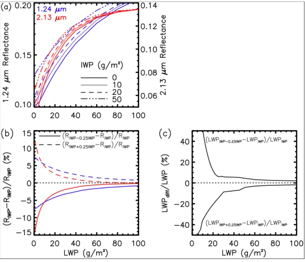
3.2 Sensitivity to IWP
To test the sensitivity of reflectances to the IWP, we first calculated the reflectances of stratiform mixed-phase clouds with four different IWP values. Fig. 5(a) shows the modeled reflectances of the 1.24 and 2.13 µm MODIS bands as a function of cloud LWP for stratiform mixed-phase clouds with IWPs of 0, 10, 20, and 50 g/m2.The other parameters used in the calculations are: re = 7.3 µm, Dge= 47.0, = 3°, 0 = 70° and = 60°. Consistent with the
theory, these figures show large contributions in the reflectance from the ice phase when the cloud LWP < 50 g/m2, and as the LWP increases, although the total reflectance is mainly from the liquid layer. However, the cloud LWP in Arctic mixed-phase clouds are small (more
than 50% of clouds have LWP less than 50 g/m2) [19], so the ice contributions is critical to
get reliable LWP for these mixed-phase clouds. Fig. 5(b) shows the relative reflectance change as a function of LWP for a 25% under- or over-estimation of IWP with a true value of 20 g/m2. Fig. 5(c) shows the percentage error in the retrieved LWP due to the 25% error in
the IWP. The figures show that an overestimation of IWP leads to overestimations of reflectances and an underestimation of the retrieved LWP and these errors decrease with the increasing cloud LWP. For clouds with LWP of 10 g/m2, a 25% error in the IWP of 20 g/m2leads to a> 50% error in the retrieved LWP, however, the error quickly decreases to
below 10% when the cloud LWP reaches ~ 20 g/m2.
Fig. 5.(a) Variations of MODIS 1.24 m band (blue) and 2.13 m band (red) reflectance as a function of mixed-phase cloud LWP for IWP values of 0 (thick solid), 10 (thin
solid), 20 (dashes) and 50 (dash-dot) g/m2. (b) The relative percentage errors in
calculated reflectance due to ±25% errors in IWP with a true value of 20 g/m2. (c) The
percentage errors in the retrieved LWPs due to ±25% errors in IWP with a true value of 20 g/m2
4. VALIDATION OF THE MIXED-PHASE RETRIEVAL ALGORITHM
4.1 Validation Using Operational MODIS Retrievals of Liquid Water Clouds
The first step to validate the mixed-phase retrieval algorithm is to compare liquid-only cloud properties obtained from the current retrievals (simply by setting IWP = 0) with those from the operational MODIS retrievals. The operational MODIS retrieval algorithm, as explained previously, was primarily intended for retrieval of re and in plane parallel liquid water
clouds. Thus the operational MODIS algorithm is ideally suited for retrieval of stratiform clouds over the ocean, which provides a homogeneous ocean surface. The operational MODIS retrievals were extensively validated [48-50]. With airborne in-situ data of the marine stratocumulus clouds off the coast of Chile from the Variability of the American Monsoon Systems’ (VAMOS) Ocean-Cloud-Atmosphere-Land Study Regional Experiment (VOCALS-Rex), [51] further confirmed the high accuracy of MODIS re andretrievals. Retrievals for
marine stratiform clouds over East Pacific around 20 – 30°N and 120 – 140°W are selected for the comparison.
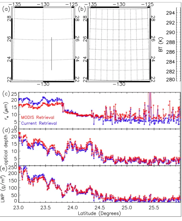
Fig. 6 shows an example of the comparison between retrievals from the current algorithm and from the operational MODIS algorithm. Fig. 6(a) and 6(b) show true color image and 11.03 µm brightness temperatures (BT), respectively. These images shows extended low level clouds over the ocean. The clouds around 22 – 24°N and 127 – 130°W have uniform cloud tops with BT ~289K. The region to the east of 130°W appears to be stratocumulus clouds with pockets of open cells (POCs). High BT (291 – 293K) in the region also confirms the existence of open water surface in the POCs region. Clouds with higher cloud tops appear around 28°N, 126°W as shown by the colder brightness temperatures. The black line in Fig. 6(a) represents the cross-section along which the results of the current retrievals are compared with the MODIS retrievals. Fig. 6(c–e) show the variations of re,and LWP along
the cross-section from south to north. The two retrievals show a good agreement and trace the increase and decrease in all the three parameters along the cross-section. For larger re,
the current retrievals show positive biases in re and negative biases in . The large re
variations that appear in both retrievals to the north of ~ 24.5°N are due to vastly non-uniform clouds or partial cloud cover in the MODIS footprint.
Fig. 7(a–c) shows the statistical comparisons of re,and LWP between the two retrievals for
the marine boundary layer clouds using data from June, 2006 (~ 1200 MODIS footprints). The diamonds represent the mean values and the vertical bars represent the 1-standard deviation of the mean within MODIS bins. The dashed curve represents the relative frequency of occurrence of the data samples. Fig. 7(a) shows that ~64% of relie in the range
of 11 -17 µm. There is a good agreement between the two retrievals with a correlation coefficient of 0.75. The current retrievals have mean biases of 1.7, 0.2 and 1.9µm relative to the MODIS retrievals for re< 11 µm, 11 µm < re< 17 µm and re> 17 µm, respectively. The
retrieved and LWP show better agreements with the MODIS retrievals, with correlation coefficients of 0.94 and 0.95 forand LWP, respectively.
Fig. 6.A case study showing cloud properties retrieved by the current algorithm and the operational MODIS algorithms for marine boundary layer clouds in the East
Pacific on July 17, 2006. (a) the MODIS true color image, (b) MODIS 11.03 m brightness temperature map, and retrieved (c) re, (d) , and (e) LWP ( red for MODIS
retrievals and blue for the current retrievals) along the cross section shown by the black line in (a).
Fig. 7.Statistical comparisons of (a) re, (b) τ and (c) LWP between the operational
MODIS retrievals and the current retrievals for warm stratiform water clouds over Eastern Pacific Ocean. The mean and the standard deviation are shown by the diamond and the vertical lines, respectively. The dot-dash lines indicate the relative
occurrence frequency of samples for each cloud properties.
4.2 Validation using Collocated Ground-Based Measurements of Mixed-Phase
Clouds
Results in section 4.1 confirm that the forward model used in the mixed-phase retrieval algorithm can achieve consistent retrievals as the operational MODIS algorithm for warm marine stratiform clouds. Here, we evaluate the algorithm performances for stratiform mixed-phase clouds with collocated ground-based multi-sensor measurements at the NSA site using measurements from March 2000 – October 2004. Since radiance measurements at visible MODIS bands are absent during winter, our analysis is restricted to measurements made between March and October. ACRF Millimeter Wavelength Cloud Radar (MMCR), Micropulse Lidar (MPL) and Microwave Radiometer (MWR) measurements and retrieved cloud properties were used to select the cases for the evaluation [22,52-54]. First, clouds are detected based on the Ze measurements from MMCR and backscatter power from MPL.
Second, deep clouds (clouds with thickness greater than 5 km), high-level clouds (clouds with bases above 5 km) and multi-layered clouds (clouds present above the mixed-phase
layer) are excluded. To ensure the maximum cloud homogeneity, the selected cases were visually screened using brightness temperature measurements from MODIS 11.03 µm. Cloudy cases with BT temperature differences > 5 K were discarded in the analysis. Third, mixed-phase cloud layers were selected based on retrieved LWP/IWP and re/Dgefor both the
liquid and the ice phases with ACRF multi-sensor measurements. Finally, we collocate available MODIS measurements with ACRF measurements and retrievals to form a collocated database for algorithm development and validations. In order to better match the surface fixed site measurements with satellite measurements, we used the following temporal and spatial averaging. The ground-based cloud properties were averaged over a 5-minute period centered at the satellite overpass time and the MODIS measurements were averaged over a region within a 3- pixel radius from the NSA site. A total of 358 cases of single layer stratiform mixed-phase clouds were selected from March 2000 to October 2004, based on the above criteria.
Because Cloud Stand CALIPSO measurements are only available in near nadir direction, the strategy of the validation with the collocated dataset is to use ground-based multi-sensor retrievals of ice phase properties (IWP and Dge) to replace 2C-ICE ice properties as inputs
for the forward-model, and then to compare MODIS retrieved LWP with ground-base LWP measurements. The ice properties are retrieved from combined MMCR and MPL measurements [52]. Although, the uncertainty for individual data points could be high, the systematic biases are small [55]. Ground-based LWP measurements are derived from two-channel MWR measurements [56]. ACRF operational MWR LWP retrievals is based on a statistical approach (hereafter referred to as ARM MWR LWP) [57], which could have high uncertainties for clouds with low LWPs and positive clear sky biases [58]. The calibration accuracy of the MWR is 0.3 K and the forward model is based on NOAA Wave Propagation Laboratory (WPL) microwave radiative transfer model described in [54,59] (here after referred as ARM-ground LWP) developed an improved statistical approach to improve low LWP retrievals from MWR measurements together with lidar determined liquid layer height and temperature. Errors in the MWR retrieved LWP are also associated with uncertainties in the dielectric properties of liquid water absorption in the microwave [60,61]. Considering these potential uncertainties, we use the two LWP retrievals to evaluate our MODIS-based mixed-phase cloud retrievals.
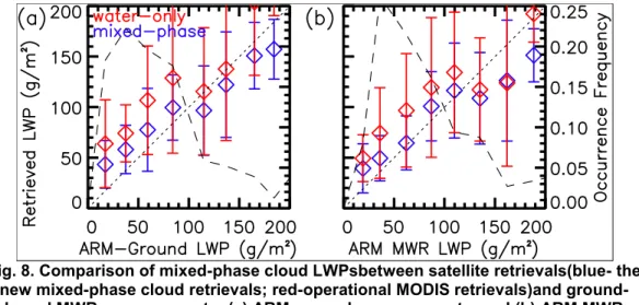
Fig. 8 shows the comparison between MODIS retrieved LWP with the ARM-ground LWP (Fig. 8(a)) and with ARM MWR LWP (Fig..8(b)) at the NSA site. The mean values of LWP (bin size of 25 g/m2) are represented by the diamonds and the vertical bars represent one
standard deviation from the mean value. The current mixed phase retrievals are shown in blue color and the operational MODIS retrievals are shown in red. Dashed curves in both the figures show the relative occurrence frequency of MWR LWPs. The LWP values vary from very low values of 5 g/m2 to values as large as 350 g/m2. However, the chance with LWP larger than ~ 200 g/m2 is very small and the data sample for these clouds is not sufficiently
large to provide statistically significant comparison due to cloud spatial in homogeneity. The frequency distribution shows that the most of the stratiform mixed-phase clouds have LWPs in the range 20 – 90 g/m2, which agrees with the results from the year-long SHEBA
campaign [15]. The figure shows that both the retrievals have high positive biases at low LWPs, however, the biases in the current mixed-phase cloud retrievals are smaller than those in the operational MODIS retrievals. One of the largest possible contributing factors for the large positive bias is the choice of surface albedo values. The NSA site is located at the northern edge of Alaska, less than a mile from the Arctic Ocean, in the fringe of the land-ocean interface. Hence, the surface albedo value can change abruptly within a short
algorithms use the 1-km 16-day average albedo, which can introduce errors in the model calculated reflectances, especially for optically thin clouds (i.e. clouds with small LWPs) as discussed above. However, the negative bias in both the mixed-phase retrievals and the operational MODIS retrievals for large LWPs cannot be due to uncertainties in the surface albedo. However, it can be attributed to uncertainties in the MWR retrievals and errors arising from temporal and spatial in homogeneities. Another source for the discrepancies between the ground-based and the retrieved LWP can be attributed to cloud in homogeneity. Although the spatial and temporal averaging is applied to the two sets of LWPs, it is still difficult to minimize the problem totally.
Fig. 8. Comparison of mixed-phase cloud LWPsbetween satellite retrievals(blue- the new mixed-phase cloud retrievals; red-operational MODIS retrievals)and
ground-based MWR measurements: (a) ARM-ground measurements, and (b) ARM MWR measurements
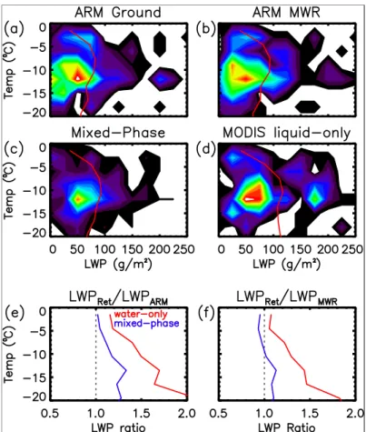
Fig. 9(a–d) shows the distributions of stratiform mixed-phase clouds in the collocated database in terms of cloud top temperature (CTT) and LWPs from different retrievals. The red curves are the mean LWP values within 3ºC temperature bins from 0 to -20ºC. The LWPs from ARM Ground, ARM MWR and the mixed-phase algorithm show similar temperature dependence, increasing LWP from 0ºC to ~ -10ºC and decreasing gradually with temperature decrease thereafter, except LWPs from the operational MODIS algorithm. When CTT gets colder than -10ºC, ice crystals are often presented in super cooled liquid layers and the ice mass fraction increases significantly as temperature decreases (Shupe et al, 2006). Therefore, ice radiative contributions in the mixed-phase clouds increase as temperature decrease. This causes the operational MODIS LWPs biased higher than other observations at colder CTTs.
Fig. 9 (e and f) show the temperature dependent LWP ratios (ratio of the satellite retrieved LWP to the MWR LWPs at the ARM NSA site). The LWP ratios are calculated separately with the ARM-ground LWPs (Fig. 9(e)) and the ARM MWR LWPs (Fig. 9(f)). Results clearly show that the LWP ratios for MODIS retrievals are larger than 1 and increase as the CTT decreases. The figures also show that the mixed phase retrievals provide significantly improved LWPs. Within the CTT range of -5 to -10ºC, the MODIS retrievals have a net positive bias of 35% in comparison to ARM-ground LWPs whereas the mixed-phase retrievals have only a net positive bias of ~ 10%. Similarly, MODIS positive biases are improved from 68% to 22% for mixed phase retrievals for clouds with CTT within 10 to -20ºC. The comparisons with the ARM MWR LWPs also show positive bias in both retrievals,
but the magnitude of the biases are smaller than those compared with the ARM-ground LWP. However, as in the case of the ARM-ground LWP, the mixed phase algorithm show marked improvements in retrieved LWPs over the operational MODIS retrieval algorithm, especially in the temperature range of -5 to -20ºC. At colder temperatures, the total water path and liquid water path are smaller and result in smaller optical depths. As a result errors from albedo uncertainties increase for colder clouds. At the same time, increasing ice fraction with decreasing CTT could result in larger errors in LWP from IWP uncertainties.
Fig. 9. Frequency distributions of stratiform mixed-phase clouds in 2-dimensional Temperature-LWP space for (a) ARM-ground, (b) ARM MWR, (c) the mixed-phase
retrieval, (d) the MODIS liquid-only retrieval. The bottom two panels show LWP ratiosbetween satellite retrievals and MWR retrievals: (e) ARM-Ground LWP and (f)ARM-MWR LWP. Blue and red colors represent the mixed-phase retrievals and the
MODIS liquid-only retrievals, respectively
5. APPLICATION TO A-TRAIN MEASUREMENTS
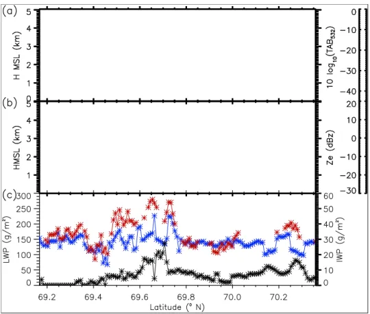
The evaluations above show that the mixed-phase algorithm can significantly improve stratiform mixed-phase cloud LWP retrievals. By combining the 2C-ICE ice cloud properties with MODIS measurements from the A-train satellite, we can apply the mixed-phase cloud algorithm globally to improve the retrievals of stratiform mixed-phase clouds. The 2C-ICE product combines CloudSat radar and CALIPSO lidar measurements to deal with lidar-only,
radar-only, and radar-lidar overlapped regions and is evaluated with large amount of in situ data [31,62]. Fig.10 shows an example of the retrievals of mixed-phase cloud with the A-Train measurements. The radar and lidar profiles show clouds extending from ~ 500 m above MSL up to 2 km. The strong signals from CALIPSO at ~ 1.5 km and the corresponding low signals from CloudSat represent a clear signature of liquid water at the top. Strong attenuation of Cloud-Aerosol Lidar with Orthogonal Polarization (CALIOP) signals by the liquid layer is also evident in Fig. 10(a). The ice virga underneath the liquid layer is shown by the Cloud Profiling Radar (CPR) Ze (Fig. 10(b)). Fig. 10(c) shows the
spatial variations of IWP and LWP of stratiform mixed-phase clouds. From the lidar and radar image, the ice virga is observed from 69.40ºN to 70.35ºN. The largest differences in the LWPs between the operational MODIS retrievals and the current mixed-phase algorithm are observed over the regions with relatively high IWPs (69.60 – 69.75ºN and 70.3ºN), with MODIS retrievals having larger LWP than the current algorithm as expected.
Fig. 10. A retrieval example of stratiform mixed-phase clouds using NASA A-train measurements. (a) CALIOP Total Attenuated Backscatter (TAB) showing a well defined water-dominated layer, (b) CPR Ze, (dBZ) showing ice virga below the
water-dominated mixed-phase layer, and (c) LWPs retrieved by operational MODIS retrievals (red) and current mixed-phase algorithm (blue). The 2C-ICE retrieved IWPs are shown
in black in (c) with labels at right side of Y-axis
Fig.11 shows statistical comparison between LWP retrievals from operational MODIS retrievals and the current mixed-phase cloud retrievals for stratiform clouds over the southern Ocean (55 - 65°S latitude) for measurements made during January 1 – 5, 2007.
These statistical comparisons show that the operational MODIS retrievals have consistent overestimation of the LWP in phase clouds when compared with the current mixed-phase cloud retrievals. Fig.11(a) shows that the positive bias in operational MODIS retrievals is larger than 50 g/m2for clouds with LWP greater than 150 g/m2. Similarly, Fig. 11(b) shows
that the LWP from operational MODIS retrievals are consistently larger and are 50% more than the LWP obtained from the current mixed phase retrievals for clouds with IWP > 10g/m2.
Fig. 11.(a) Comparison of LWP from the current mixed-phase retrievals against LWP from operational MODIS retrievals at 15 g/m2bins for marine stratiform mixed-phase
clouds in the Southern Ocean. The means and the standard deviations are shown by triangles and vertical lines, respectively. (b) The LWPs from operational MODIS retrievals (red) and the current mixed-phase retrievals (blue) as a function of IWP. The
means and the standard deviations are shown by triangles and horizontal lines, respectively. The black curve represents LWP ratio (LWPMODIS/LWPCurrent).
6. SUMMARY AND CONCLUSION
A mixed-phase cloud retrieval algorithm was developed for stratiform mixed-phase clouds by using multi sensor measurements from the NASA A-Train satellites. Similar to the operational MODIS algorithm, the following main assumptions were used in the forward model: (1) plane-parallel atmosphere with a liquid water layer over an ice layer representing stratiform mixed-phase clouds. This simple stratiform mixed-phase cloud structure is confirmed by extensive ground-based active and passive measurements. (2) The surface is Lambertian with the surface albedo changing in a 16-day cycle based on MODIS measurements. (3) Rayleigh scattering by atmospheric molecules is negligible at wavelengths longer than 1 m. Reflectance measurements at one non-absorbing and another absorbing (in relation to liquid and ice) MODIS bands were compared to the model calculated reflectance using DISORT with known ice properties from CPR and CALIOP measurements to simultaneously retrieve liquid-phase reand combination that minimized
the difference between the observations and model calculations. LWP was calculated from the combination of re and .The error analyses suggest that retrieval accuracy of LWP is
highly dependent on the accuracies of the surface albedo and IWP used for radiative calculations when LWP < 30g/m2.
First, the mixed-phase algorithm was tested by comparing the retrievals with the operational MODIS retrievals for warm marine stratiform clouds over Eastern Pacific Ocean by setting IWP as zero in the algorithm. Brightness temperature measurements from MODIS 11.03 µm band were used to avoid the presence of clouds above the stratiform deck. The comparison showed good statistical agreements in reandbetween the current retrieval method and the
operational MODIS algorithm, with correlation coefficient of 0.75and 0.94 for re and ,
respectively. The retrieved LWPs had a correlation coefficient of 0.95. A positive bias was observed for LWPs larger than ~ 300 g/m2, which increased with increasing LWP values.
Then, the retrieval algorithm was applied to stratiform mixed-phase clouds observed at the NSA site and was validated with collocated ground-based multi-sensor measurements. Because CPR and CALIOP get really close to the NSA site, ground-base lidar-radar retrievals of IWP and Dgewere used together with MODIS measurements to retrieve LWP for
these mixed-phase clouds. The satellite retrieved LWPs were compared with LWPs from ground MWR measurements. Results show that the operational MODIS LWP retrievals are prone to large positive bias in the temperature range of – 5 to – 20ºC when treating the mixed-phase clouds as liquid-only clouds in these temperatures [61]. The mixed-phase algorithm provides better LWP retrievals than the operational MODIS retrievals when compared with the ground-based measurements, although there are still positive biases. The positive LWP biases were improved from 35% to 10% and 68% to 22% for mixed phase clouds with CTT ranges of -5 to -10ºC and -10 to -20ºC, respectively. The differences in the radiative properties of ice and water are the main reason that causes errors in the operational MODIS retrievals that assume liquid-only clouds for mixed-phase clouds. As a result, attributing the reflected radiation to water droplets result in the retrieved LWP as being different to not only the actual LWP, but to the cloud water path (sum of liquid water path and ice water path) as well.
Finally, the algorithm was applied to stratiform mixed-phase clouds observed by the A-train satellites. The ice properties from the 2C-ICE product were combined with MODIS measurements to retrieve liquid-phase properties for stratiform mixed-phase clouds. Case studiesof mixed-phase clouds in the Arctic region and statistical comparison of mixed-phase clouds in the Southern Ocean by using a large dataset (~ 2500 MODIS footprints) showed that the algorithm provides expected improvements compared with operational MODIS retrievals. We will build a more universal look-up table to apply the algorithm to multi-year A-train measurements to provide reliable LWPs for stratiform mixed-phase clouds on the global scale. Mean while, we have to explore other options with satellite measurements to improve the retrieval accuracies for optically thin mixed-phase clouds.
ACKNOWLEDGEMENTS
This research was funded by NASA grant NNX10AN18G and also partially supported by DOE DE-SC0006974 as part of the ASR program. We thank the CALIPSO and CloudSat data group for providing high quality data. Surface remote sensing data were obtained from the ARM program sponsored by the U.S. Department of Energy, Office of Science, Office of Biological and Environmental Research and Environmental Sciences Division.
COMPETING INTERESTS
REFERENCES
1. Giovinetto MB, Yamazaki K, Wendler G, Bromwich DH. Atmospheric net transport of water vapor and latent hear across 60°S.J Geophys Res.1997;102(D10):11171– 11179.
2. Slonaker RL, Van Woert ML. Atmospheric moisture transport across the Southern Ocean via satellite observations, JGeophys Res.1999;104(D8):9229–9249.
3. Liou KN. Influence of cirrus clouds on weather and climate processes: A global perspective. Mon Wea Rev. 1986;114:1167–1199.
4. Ramanathan V, Cess RD, Harrison EF, Minnis P, Barkstrom BR, Ahmad E, et al.. Cloud-radiative forcing and climate: Results from the Earth Radiation Budget Experiment.Science.1989;243,57–63.
5. Stephens GL. Cloud feedback in the climate system: A critical review.J Climate. 2005;18:237–273.
6. Hogan RJ, Francis PN, Flentje H, Illingworth AJ, Quante M, Pelen J. Characteristics of mixed-phase clouds. I: Lidar, radara and aircraft observations from CLARE’ 98.Q J R Meteorol Soc. 2003;129:2089-2116.
7. Luo Y, Xu KM, Morrison H, McFarquhar G. Arctic mixed-phase clouds simulated by a cloud-resolving model: Comparison with ARM observations and sensitivity to microphysics parameterizations. J Atmos Sci. 2008;65:1285-1303, doi:10.1175/2007JAS2467.1.
8. Shupe MD, Daniel JS, De Boer D, Eloranta EW, Kollias P, Long CN, et al.. A focus on mixed-phase clouds: The status of ground-based observational methods. BAMS.2008;10:1549-1562.
9. Sassen K, Liou KN, Kinne S, Griffin M. Highly super cooled cirrus cloud water: Confirmation and climate implications. Science.1985;227:411–413.
10. Heymsfield AJ, Miloshevich LM. Homogeneous ice nucleation and super cooled liquid water in orographic wave clouds. J Atmos Sci.1993;50(15):2335–2353.
11. Pruppacher HR. A new look at homogeneous ice nucleation in supercooled water drops. J Atmos Sci. 1995;52(11):1924–1933.
12. Rosenfeld D, Woodley WL. Deep convective clouds with sustained supercooled liquid water down to -37.5°C.Nature. 2000;405:440–442.
13. Fan J, Ghan S, Ovchinnikov M, Liu X, Rasch PJ, Korolev A. Representation of Arctic mixed-phase clouds and the Wegener-Bergeron-Findeisen process in climate models: Perspectives from a cloud resolving study. J Geophys Res. 2011;116,D00T07, doi:10.1029/2010JD015375.
14. Turner DD. Arctic mixed-phase cloud properties from AERI lidar observations: Algorithm and results from SHEBA. J Appl Meteor. 2005;44:427-444.
15. Shupe MD, Matrosov SY, Uttal T. Arctic Mixed-phase cloud properties derived from surface-based sensors at SHEBA. J Atmos Sci. 2006;63:697–711.
16. Zhang D, Wang Z, Liu D. A global view of midlevel liquid-layer topped stratiform cloud distribution and phase partition from CALIPSO and CloudSat measurements. J Geophys Res. 2010;115,D00H13, doi:10.1029/2009JD012143.
17. De Boer G, Collins WD, Menon S, Long CN. Using surface remote sensors to derive radiative characteristics of mixed-phase clouds: an example from M-PACE. Atmos Chem Phys. 2011;11:11937–11949.
18. Klein SA, McCoy RB, Morrison H, Ackerman AS, Avramov A, de Boer G, et al. Intercomparison of model simulations of mixed-phase clouds observed during the ARM Mixed-Phase Arctic Cloud Experiment. I: Single-layer cloud. Q J R Meteorol Soc. 2009;135:979-1002.
19. Zhao M, Wang Z. Comparison of Arctic clouds between European Center for Medium-Range Weather Forecasts simulations and Atmospheric Radiation Measurement Climate Research Facility long-term observations at the North Slope of Alaska Barrow site. J Geophys Res. 2010;115,D23202, doi:10/1029/2010JD014285.
20. Vavrus S. The impact of cloud feedbacks on Arctic climate under greenhouse forcing.J Climate.2004;17:603–615.
21. Tsushima Y, Emori S, Ogura T, Kimoto M, Webb MJ, Williams KD, et al. Importance of the mixed-phase cloud distribution in the control climate for assessing the response of clouds to carbon dioxide increase: a multi-model study. Climate Dynamics.2006;27:113-126.
22. Wang Z, Sassen K, Whiteman DN, DemozBB.Studying Altocumulus with ice virga using ground-based active and passive remote sensors. J Appl Meteor.2004;43:449-460.
23. Shupe MD, Uttal T, Matrosov SY. Arctic cloud microphysics retrievals from surface-based remote sensors at SHEBA.J Appl Meteor.2005;44:1544-1562.
24. King MD, Kaufman YJ, Menzel WP, Tanré D. Remote sensing of cloud, aerosol, and water vapor properties from the Moderate Resolution Imaging Spectrometer (MODIS), IEEE TransGeosci Remote Sensing. 1992;30:2–27.
25. King MD, Menzel WP, Kaufman YJ, Tanré D, Gao B-C, Platnick S, et al. Clouds aerosol properties, precipitable water, and profiles of temperature and water vapor from MODIS, IEEE Trans Geosci Remote Sensing. 2003;41:442–458.
26. Platnick S, King MD, Ackerman SA, Menzel WP, Baum BA, Riedi JC, et al. The MODIS cloud products: Algorithms and examples from Terr., IEEE Trans Geosci Remote Sensing. 2003;41:459–473.
27. Lee J, Yang P, Dessler AE, Baum BA, Platnick S. The influence of thermodynamic phase on the retrieval of mixed-phase cloud microphysical and optical properties in the visible and near infrared region. IEEE Trans Geosci Remote Sensing. 2006;3(3):287-291.
28. Ou SSC, Liou KN, Wang XJ, Hagan D, Dybdahl A, Mussetto M, et al. Retrievals of mixed-phase cloud properties during the national polar orbiting operational environmental satellite system. Appl Optics. 2009;48(8):1452-1462.
29. Austin RT. Level 2B radar-only cloud water content (2B-CWC-RO) process description document. 2007; Accessed November 29, 2012. Available: http://www.cloudsat.cira.colostate.edu/ICD/2B-CWC-RO/2B-CWC-RO_PD_5.1.pdf. 30. Austin RT, Heymsfield AJ, Stephens GL. Retrieval of ice cloud microphysical
parameters using the CloudSat millimeter-wave radar and temperature. J Geophys Res. 2009;114,D00A23, doi:10.1029/2008JD010049.
31. Deng M, Mace GM, Wang Z, Okamoto H. Tropical composition, cloud and climate coupling experiment validation for cirrus cloud profiling retrieval using CloudSat radar and CALIPSO lidar, J Geophys Res. 2010;115,D00J15, doi:10.1029/2009JD013104. 32. Hansen JE, Travis LD. Light scattering in planetary atmospheres. Space Sci Rev.
1974;16:527–610.
33. King MD, Tsay S-C, Platnick S, Wang M, Liou KM. Cloud retrieval algorithms for MODIS: Optical thickness, effective particle radius, and thermodynamic phase, Algorithm Theor Basis Doc. ATBDMOD-05. 1997. Accessed November 29, 2012. Available: http://modis-atmos.gsfc.nasa.gov/_docs/atbd_mod05.pdf.
34. Schaaf CB, Gao F, Strahler AH, Lucht W, Li X, Tsang T, et al. First operational BRDF, albedo nadir reflectance products from MODIS. Remote Sens Environ. 2002;83:135-148.
35. Intrieri JM, Fairall CW, Shupe MD, Persson POG, Andreas L, Guest PS, et al.An annual cycle of Arctic surface cloud forcing at SHEBA. J Geophys Res. 2002;107(C10):8039, doi:10.1029/2000JC000439.
36. Verlinde J, Harrington JY, McFarquhar GM, Yannuzzi VT, Greenberg S, Johnson N, et al.The Mixed-Phase Arctic Cloud Experiment. Bull Amer Meteor. Soc. 2007;2:205– 221.
37. Stamnes K, Tsay S-C, Wiscombe W, Jayaweera K. Numerically stable algorithm for discrete ordinate radiative transfer in multiple scattering emitting layered media. ApplOptics. 1988;27(12):2502–2509.
38. Stamnes K, Tsay SC, Wiscombe W, Laszlo I. DISORT, a general purpose fortran program for discrete-ordinate method radiative transfer in scattering and emitting layered media: Documentation and methodology, report. 2000; Available:
http://www.met.reading.ac.uk/~qb717363/adient/rfm-disort/DISORT_documentation.pdf.
39. King MD, Radke LF, Hobbs PV. Determination of the spectral absorption of solar radiation by marine stratocumulus clouds from airborne measurements within clouds. J Atmos Sci. 1990;47(7):894-907.
40. Palmer KF, Williams D. Optical properties of water in the near infrared. J Optical Soc America. 1974;64(8):1107-1110.
41. Downing HD, Williams D. Optical constants of water in the infrared. J Geophys Res. 1975;80(12):1656-1661.
42. Yang P, Liou KN, Wyser K, Mitchell D. Parameterization of the scattering and absorption properties of individual ice crystals. J Geophys Res. 2000;105(D4):4699-4718.
43. Hallet J, Mason BJ. The influence of temperature and super saturation on the habit of ice crystals grown from the vapour. Proc Roy Soc London. 1958; 247A:440–453. 44. Keller VW, Hallett J. Influence of air velocity on the habit of ice crystal growth from
vapor. J Crystal Growth. 1982;60:91–106.
45. Bailey MP, Hallett J. Nucleation effects on the habit of vapour grown ice crystals from -18°C to -42°C. Quart J Roy Meteor Soc. 2002;128:1461–1483.
46. Fu Q. An accurate parameterization of the solar radiative properties of cirrus clouds for climate models. J Climate. 1996;9:2058–2082.
47. Han Q, Rossow WB, Chou J, Welch RM. Global survey of the relationships of cloud albedo and liquid water path with droplet size using ISCCP. J Climate. 1998;11:1516-1528.
48. Mace GG, Zhang Y, Platnick S, King MD, Minnis P, Yang P. Evaluation of cirrus cloud properties derived from MODIS data using cloud properties derived from ground-based observations collected at the ARM SGP site. J Appl Meteor. 2005;44:221-240. 49. Varnai T, Marshak A. View angle dependence of cloud optical thickness retrieved by
Moderate Resolution Imaging Spectroradiometer (MODIS). J Geophys Res. 2007;112: D06203, doi:10.1029/2005JD006912.
50. Seethala C, Horvath A. Global assessment of AMSR-E and MODIS cloud liquid water path retrievals in warm oceanic clouds. J Geophys Res. 2010;115,D13202, doi:10.1029/2009JD012662.
51. Painemal D, Zuidema P. Assessment of MODIS cloud effective radius and optical thickness retrievals over the Southeast Pacific with VOCALS-REx in situ measurements. J Geophys Res.2011;116, D24206,doi:10.1029/2011JD016155. 52. Wang Z, Sassen K. Cirrus cloud microphysical property retrieval using lidar and radar
measurements. Part I: Algorithm description and comparison with in situ data. J Appl Meteor. 2002;41:218-229.
53. Wang Z, Sassen K. Cirrus cloud microphysical property retrieval using lidar and radar measurements. Part II: Midlatitude cirrus microphysical and radiative properties. J Atmos Sci. 2002;59:2291-2302.
54. Wang Z. A refined two-channel microwave radiometer liquid water path retrieval for cold regions by using multiple-sensor measurements. IEEE Geoscience & remote sensing letts. 2007;4:591-595.
55. Heymsfield AJ, Protat A, Austin RT, Bouniol D, Hogan RJ, Delanoe J, et al. Testing IWC retrieval methods using radar and ancillary measurements with in situ data. J Appl Meteor.2008; 47:135-163.
56. Westwater ER. The accuracy of water vapor and cloud liquid determination by dual-frequency ground-based microwave radiometry. Radio Sci. 1978;13(4):677-685. 57. Lilgegren JC, Clothiaux EE, Mace GG, Kato S, Dong XQ.A new retrieval for cloud
liquid water path using a ground-based microwave radiometer and measurements of cloud temperature. J Geophys Res. 2001;106(D13):14485-14500.
58. Marchand R, Ackerman T, Westwater ER, Clough SA, Cady-Pereira K, Liljegren JC. An assessment of microwave absorption models and retrievals of cloud liquid water using clearsky data. J Geophys Res. 2003;108(D24):4773-4782,doi:10.1029/2003JD003843.
59. Schroeder JA,Westwater ER. User’s guide to WPL microwave radiative transfer software, NOAA Tech. Memo., ERL WPL-213, NOAA ERL Wave Propagation Lab., Boulder, Co. 1991.
60. Matzler C, Rosenkranz PW, Cermak J. Microwave absorption of supercooled clouds and implications for dielectric properties of water, J Geophys Res., 2010;DOI 10.1029/2010JD014283.
61. Cadeddu MP, Turner DD. Evaluation of water permittivity models from ground-based observations of cold clouds at frequencies between 23 and 170 GHz, IEEE Trans Geosci Remote Sensing. 2011:8:2999-3008.
62. Deng M, Mace GG, Wang Z, Lawson RP. Testing and evaluation of ice water content retrieval methods using radar and ancillary measurements, J Appl Meteor. 2012; (In press).
Appendix A:
r
e(m) values used in the forward model:
3.1, 4.2, 5.2, 6.3, 7.3, 8.4, 9.4, 10.4, 11.5, 12.5, 13.6, 14.6, 15.7, 16.7, 17.7, 18.8,
19.8, 20.86, 21.9, 23.0, 24.0, 25.0, 26.1, 27.1, 28.2, 29.2, 30.3, 31.3, 32.3, 33.4,
34.4, 36.4
___________________________________________________________________
© 2013 Adhikari and Wang; This is an Open Access article distributed under the terms of the Creative Commons Attribution License (http://creativecommons.org/licenses/by/3.0), which permits unrestricted use, distribution, and reproduction in any medium, provided the origin al work is properly cited.
Peer-review history:
The peer review history for this paper can be accessed here: http://www.sciencedomain.org/review-history.php?iid=323&id=10&aid=2532