Analytical and Experimental Vibration Analysis of Glass Fibre Reinforced Polymer Composite Beam

Full text

(1)Master's Degree Thesis ISRN: BTH-AMT-EX--2007/D-13--SE. Analytical and Experimental Vibration Analysis of Glass Fibre Reinforced Polymer Composite Beam. Oluseun Adediran. Department of Mechanical Engineering Blekinge Institute of Technology Karlskrona, Sweden 2007 Supervisor:. Ansel Berghuvud, Ph.D. Mech. Eng..

(2)

(3) Analytical and Experimental Vibration Analysis of Glass Fibre Reinforced Polymer Composite Beam Oluseun Adediran Department of Mechanical Engineering Blekinge Institute of Technology Karlskrona, Sweden 2007 Thesis submitted in fulfilment of the completion of Master of Science in Mechanical Engineering by the Department of Mechanical Engineering, Blekinge Institute of Technology, Karlskrona, Sweden. Abstract: The aim of this work is to investigate analytical and experimental vibration of composite beam. The composite beam is used as composite footbridge model prototype which is assumed. For the dynamic test, hammer excitation is used to excite the beam at fixed locations. The modal parameters are extracted from the time response using a time domain analysis, i.e. the stochastic subspace identification technique. Finite element models for different boundary conditions are constructed using the commercial finite element software package ANSYS for natural frequencies of the beam to support and verify the dynamic measurements. The result obtained from analytical solution, dynamic tests and the FEM are presented and analysed. Keywords: Modal Parameters, Frequency, Mode shapes, FE Model, Composite Beam Structure..

(4) Acknowledgements This work was carried out under the supervision of Dr Ansel Berghuvud, Blekinge Institute of Technology, Karlskrona, Sweden and Dr. Abdel Wahab University of Surrey, United Kingdom I wish to express my gratitude to a lot of people who have supported me during the past years in one way or the other. To my major professor, Dr. Abdel Wahab, a special thanks for giving me the opportunity to work with him and for his patience, tolerance, understanding, and encouragement. He was more than a professor to me; he was also a friend. It has been a great pleasure working with him. I wish to thank Dr Ansel Berghuvud. I am very thankful to my research group members, Prof Andrew Crocombe, Mr Libardo, Irfan for their patience, and advice. I really appreciate their time and effort in being part of my research group. Thanks are also extended to Mr & Mrs Sola Olalekan, Olanrewaju, Sogo, Opeyemi, Anuoluwapo, Ebunoluwa, Oluwole for their support and help in many ways. I also want to thank all those that helped me through the research. The greatest thanks go my mother for her financial support throughout my degree programme. A special thanks to my loving mother, for being there for me all the time of my needs. Also, I thank my friend Babatunde Rasheed. I am very grateful to my wife, Oluwatoyin, for her encouragement. She brought more love and strength to my life.. Karlskrona, October 2007 Oluseun. A. Adediran. 2.

(5) Contents 1 Notations. 5 . 2 Introduction 2.1 Research Context 2.2 Objectives 2.3 Review of previous work 2.3.1 Composite Materials FRP for Bridge Applications 2.3.2 Recent Research in FRP 2.3.3 Characteristics of FRP Structural Beam 2.3.4 Problem with Composite Material 2.3.5 Advantages of Composite Beam 2.3.6 Disadvantages of FRP Composite Beam 2.3.7 Applications of FRP Composite Beam. 8 8 9 10 10 12 14 15 15 16 16 . 3 Basic Concepts and Theory 3.1 Structural dynamics 3.1.1 SDOF model 3.1.2 MDOF model 3.2 Experiment Modal analysis 3.2.1 Introduction 3.2.2 Theoretical Derivation. 17 17 17 18 19 19 20 . 4 Beam Structure 4.1 Introduction 4.2 Finite Element Method Calculations. 23 23 25 . 5 Experimental Work 5.1 Introduction 5.1.1 Measurement Preparations 5.1.2 Identification of Experimental Model 5.1.3 Position of the Accelerometer on the Beam 5.1.4 Point of Excitation 5.2 FRP Composite Beam Test Descriptions 5.3 Measurement Equipment 5.3.1 Data acquisition system 5.3.2 Accelerometer 5.3.3 Impact Hammer 5.3.4 Steel Support 5.3.5 PC with Software. 31 31 31 31 32 32 33 35 35 36 36 37 38 . 3.

(6) 5.4 Experimental Specifications 5.5 . 38 . Experimental Results and Discussion 5.5.1 Results. 40 40 . 6 Modelling in ANSYS 6.1 Introduction 6.2 Procedure in Modelling ANSYS 6.2.1 Requirement Specification 6.2.2 Idealization Specification 6.2.3 Mesh Generation 6.2.4 Analysis 6.2.5 Post-processing 6.3 ANSYS Graphical Results 6.3.1 Simple-Simple Boundary Condition 6.3.2 Fixed-Fixed Boundary Condition 6.3.3 Fixed-Simple Boundary Condition 6.3.4 Fixed-Free Boundary Condition. 47 47 48 48 49 49 50 50 50 50 52 53 55 . 7 Discussion 7.1 Introduction 7.2 Comparison of Method 7.3 Effect of Boundary Conditions on Natural frequency. 57 57 57 60 . 8 Conclusion 8.1 Future Work. 61 61 . 9 References. 62 . Appendices 1 Terminology 2 Calculation of FEM Natural frquencies of beam (1 element) 3 Calculation of FEM Natural frquencies of beam (2 element). 64 64 66 69. 4.

(7) 1. Notations. List of symbols C1 , C 2 , C 3 , C 4 Constant-time function in the model C. Wave equation for the beam. ai. AR matrix parameters. F(t). excitation force at time t. F. frequency [Hz]. E. Young Modulus. fs. Elastic force exerted on the mass. fD. Damping force. fI. Inertial force of the mass. H (ω ) Frequency response function I. moment of inertia. M, Cp, K. mass, damping and stiffness matrix. z (t ), z& (t ), &z&(t ) Displacement, velocity and acceleration vectors at time t. ξ. Damping ratio. ψ. Mode shapes. u&&. Acceleration. u&. Velocity. u. Displacement. φn. Modes. ωn. Natural frequency. βnL. Constant value. FI. external forces. 5.

(8) ρ. Density of the beam. T. Kinetic Energy. Vy. Velocity in y-direction. ω. Angular frequency [rad/s]. ρ. Density of the composite beam [kg/m3]. Uj. Nodal degree of freedom at nodes j. Ui. Nodal degree of freedom at nodes i. Mi. Bending moment acting at node i. Mj. Bending moment acting at node j. Fi. External forces. W. Strain Energy. List of operator. (⋅) T ~ (). Generalised System. (⋅) −1. matrix inverse. (⋅) *. complex conjugate. (⋅) i. data or estimate from patch i. Re (⋅). real part of. Im (⋅). imaginary part of. matrix transpose. 6.

(9) List of abbreviations. DOF. Degree of Freedom. SDO. Single Degree of Freedom. MDOF. Multiple Degree of Freedom. EMA. Experimental Modal Analysis. EMT. Experimental Modal Testing. FE. Finite Element. N/A. Not Available. FEM. Finite Element Method. FFT. Fast Fourier Transform. FRF. Frequency Response Function. PP. Peak Picking. RMS. Root.Mean Square. NDT. Non-Destructive Testing. FRP. Fibre reinforced Polymer/Plastic. GFRP. Glass Fibre reinforced Polymer/Plastic. 7.

(10) 2. Introduction. This chapter contains a general introduction of the research that was carried out within the frame work of this thesis. The research context is described in Sec.2.1. The focus of the thesis as well as the main objectives is discussed in Sec.2.2.. 2.1 Research Context The beam is manufactured from a Glass Fibre Reinforced Plastic (GFRP) and its box like beam. This beam was actually used as a prototype for footbridge. The GFRP (Glass Fibre Reinforced Polymer) composite materials are being utilised in more structures like bridges as the technology and understand of them improves. GFRP composite are ideal for structural applications where high strength to weight and stiffness to weight ratios are needed. As the technology progresses, the cost involved in manufacturing and designing composite material will reduce, thus bringing added cost benefits also. The vibration analyses in footbridge have been a problem for structural designer for years and have increased recently. The trend in footbridge design has been towards greater spans and increased flexibility and lightness. Though, many of our footbridges have natural frequencies with the potential to suffer excessive vibrations under dynamic load induced by pedestrians. However, as with any structure, the loading upon it will need to be considered so that it can perform as intended when it is commissioned for the usage. This is done by using modal analysis, which allows one to determine the natural frequencies of the structure, associated mode shapes and damping. And once natural frequencies are known, thus making structure suitable for the task designed for. This is mainly due to the human feeling of vibration while crossing a footbridge with a frequency close to the first (fundamental) natural frequency of the bridge, although the vibration caused by the pedestrians are far from harmful to the bridge. Therefore vibration analysis of such structure can be considered to be a serviceability issue. Modal parameters of a structure are frequency, mode shape and damping. Frequency is directly proportional to structure’s stiffness and inverse of mass.. 8.

(11) Nevertheless, modal parameters are functions of physical properties of the structure. Thus, changes in the physical properties such as, beginning of local cracks and/or loosening of a connection will cause detectable changes in the modal properties by reducing the structure’s stiffness. The design of GFRP (Glass Fibre Reinforced Polymer) bridge deck established to promote the use of innovative material and lead to use in footbridge construction to improve the reliability for proper safety and serviceability. The Aberfeldy cable-stayed was the first GFRP footbridge, built back in 1992. There are only two GFRP footbridge existing in UK knows as the Halgavor and Willcot [1&2]. The use of glass or carbon fibre reinforced polymer was due to its advantages, for they are easily drawn into having a high strength-to-weight ratio, low maintenance and lightweight. In this research, Finite element models for different boundary conditions are constructed using the commercial finite element software package ANSYS to support and verify the dynamic measurements. Initial a FE 3D model of FRP (Fibre Reinforced Polymer) composite beam was created without curvature using beam elements. Furthermore, the FE results of the straight beam are compared to the exact solution obtained from analytical solution for understanding of the relationship between the FE results. The natural frequencies and modes shapes of the composite beam are obtained after performing modal analysis which the author contribution to this area of research.. 2.2 Objectives The main objective of this thesis is to study and compare the analytical and experimental result in vertical forces on the composite Fibre Reinforced Polymer (FRP) beam. The beam assumed as prototype of bridge in which pedestrians impart to the model. Special attention is given to the responses of a structure due to dynamic test (impact excitation) results compare with theoretical results. The GFRP (Glass Fibre Reinforced Polymer) composite beam was used to carry out good experimental research, for comparison of the results, and to be able to relate to the reality of the footbridge built with composite beam.. 9.

(12) 2.3 Review of previous work 2.3.1. Composite Materials FRP for Bridge Applications. Many researchers have worked on composite material especially in the constructions of bridges. The first pedestrian FRP bridge was built by the Israelis in 1975. Since then, others have been constructed in Asia, Europe, and North/South America. Many innovative pedestrian bridges have been constructed throughout the Europe especially United Kingdom using protruded composite structural shapes which are similar to standard structural steel shapes. Because of the lightweight materials and ease in fabrication and installation, many of these pedestrian bridges were able to be constructed in inaccessible and environmentally restrictive areas without having to employ heavy equipment [3]. Some of these bridges were flown to the sites in one piece by helicopters; others were disassembled and transported by mules and assembled on site. The advancement in this application has resulted in the production of second generation protruded shapes of hybrid glass and carbon FRP (Fibre Reinforced Polymer) composites that will increase the stiffness modulus at very little additional cost. The recognition of providing high quality fibres at the most effective regions in a structural member’s cross section is a key innovation to the effective use of these high performance materials. With the knowledge gained from working with pedestrian bridges, many researchers took the next step toward designing FRP composite vehicular bridges. Many deck systems were developed and tested beginning in the early 1990's. there are no many FRP bridges around the world, we have only know of two completed bridges in United Kingdom, Halgavor (firth 2002) and Wilcott which is most recent one. The first world all-composite vehicular, public bridge was placed in service on 1992 in Aberfeldy. It was a wet lay-up manufacturing method, a technology transfer from the defence industry. The FRP (Fibre Reinforced Polymer) deck panels were shopfabricated with composite honeycomb cells sandwiched between two face sheets. It became a common material for construction of deck after the first US in 1996, Kansas. FRP (Fibre Reinforced Polymer) composites have a high tensile strength; however, in almost all of the demonstration bridge projects constructed to date, the design has been driven by the stiffness rather than strength. There is still much room for improvement and advancement of the composite deck systems in order to capitalize on its material strength.. 10.

(13) The key to successful application of the deck superstructure system is to optimize its geometric cross section and to establish well-defined load paths. Because most of these deck systems are sealed and enclosed, they are inaccessible for field inspection. To ensure the composites integrity, sophisticated non-destructive evaluation/testing (NDE/NDT) devices and fibre optic sensors have been incorporated into some of the composite deck systems to monitor the in-service condition of and the presence of moisture in the bridge deck. With time the effectiveness of the monitoring systems and the long-term service performance of composites can be ascertained. The modular panel construction of bridge deck systems enables quick project delivery. A bridge built of composite materials can be constructed and put in service in a relatively short time and at a competitive cost. Its lightweight materials and ease of construction provide tremendous labour and traffic control cost savings to offset a higher first cost. An FRP deck could reduce the weight of conventional construction by 70 to 80 percent. This technology has demonstrated that a bridge structure can be replaced and put into service in a matter of hours rather than days or months. The conveniences is replacing composite bridges is comparable, it is due to innovative technology put to good use. The FRP composites offer the potential to eliminate the problem of excessive dead load of long span bridges. Structural components for hybrid bridge construction such as FRP (Fibre Reinforced Polymer) reinforcing elements, cable and tendon systems, and laminates have been successfully demonstrated in highway bridges. The reinforcing elements are fabricated into 1-D rods, 2-D grids or gratings, and 3-D fabric or cage systems. The application of composite materials to infrastructure has been limited due to the lack of industry-recognized design criteria and standards and standardized test methods [4] Cable and tendon systems are subject to fatigue, and under sustained loads will creep. Creep rupture is a major concern for glass fibres. Proper selection of fibres and adequate design criteria must be established to ensure the proper use of these products and are essential to the advancement of FRPs in pre-stressing applications. Laminates are protruded with unidirectional fibres to form thin and narrow plates There is much work to be done in developing well-designed anchorages, connection details, and bonded joints in composites for long-term. 11.

(14) durability. Bridge engineers are reluctant to rely solely on epoxy adhesive bonding technology to connect or join structural components. Electrical transmission towers out West have been built with connections that were snapped and locked together without the use of any fasteners. It is a tough challenge, but when adequate testing and performance data are available, bridge engineers will change their paradigm. Since, thousands of concrete bridge piers that were designed with inadequate ductility, lap splices, and shear capacity have been successfully retrofitted using FRP (Fibre Reinforced Polymer) composite wrap systems. In Cali it has been determined that when a wrap system is properly designed and installed, the ductile capacity can be significantly increased to allow twice the deformation levels without any reduction in its capacity as compared to the as-built bridge piers[5]. Several countries have successfully applied FRP (Fibre Reinforced Polymer) composite materials to the repair of damaged or deteriorated beams in highway bridges. With this application, the condition of the deterioration in the concrete behind the composite materials remains uncertain. A good repair program should include an evaluation of the preexisting condition and structural integrity of the concrete to establish a baseline reference. After a structural member has been repaired, the inservice condition of the concrete substrate as well as the performance of the composites should be continuously followed up.. 2.3.2. Recent Research in FRP. Research studies and results of the composite technology and its durability should be published in civil, mechanical and structural engineering journals. Technical papers should be presented in conferences and workshops where civil and structural engineers participate. Until recently, most of the papers have been published in the materials science and testing, manufacturing and trade journals, which are not read by bridge designers. Information and knowledge must be openly shared with civil engineers, bridge designers, and owners. Professional organizations should be dedicated and/or established to direct the technical advancement of the composite technology if it is to have a future. Composite material bridges have become increasingly popular in structural applications around the world. This is partly due to their excellent. 12.

(15) earthquake-resistant properties such as high strength, high ductility, and large energy absorption capacity. Although the risk of a major earthquake in United Kingdom is small, this type of structure can offer many other advantages, for instance the increased speed of construction; positive safety aspects; the steel tube's function as both formwork and reinforcement for the concrete core; and possible use of simple standardized connections. Today's possibility to produce composite with higher compressive strength allows the design of more slender columns, which leads to greater profits. To prevent the brittle failure that is normally associated with-high strength deck and obtain a higher ductility, the stirrup spacing is often decreased. A lot of work is needed in material science development and production. Design and construction specifications are important protocol for engineers, and they need to be developed. Bridge owners must know how to inspect, maintain, and repair FRP (Fibre Reinforced Polymer) composite bridges and these procedures must be established. We need to involve more knowledgeable and experienced engineers to help develop standards, design guidelines, and specifications. This is an exciting time for civil and structural engineers to be involved with the FRP (Fibre Reinforced Polymer) composite technology. Although most engineers are not trained to work with fibre and resin composite materials, they can quite easily pick up the knowledge. Education and training should be provided to the critical mass of practicing engineers. Research studies and results of the composite technology and its durability should be published in civil and structural engineering journals. Technical papers should be presented in conferences and workshops where civil and structural engineers participate. Until recently, most of the papers have been published in the materials science and testing, manufacturing and trade journals, which are not read by bridge designers. Information and knowledge must be openly shared with civil engineers, bridge designers, and owners. Professional organizations should be dedicated and/or established to direct the technical advancement of the composite technology if it is to have a future [6]. There is still more work needed in material science development and production. Design and construction specifications are important protocol for engineers, and they need to be developed. Bridges owners must know how to inspect, maintain, and repair Fibre Reinforced Polymer (FRP) composite bridges and these procedures must be established.. 13.

(16) We need to involve more knowledgeable and experienced engineers to help develop standards, design guidelines, and specifications when we have an approved design standard specifications for FRP (Fibre Reinforced Polymer) composites. 2.3.3. Characteristics of FRP Structural Beam. Nagaraj and Rao [7] have characterized the behaviour of protruded FRP box beams under static and fatigue or cyclic bending loads. The author showed that the shear and interfacial slip between adjacent layers had significant influence on deflection and strain measurements. Davalos and Qiao [8] conducted a combined analytical and experimental evaluation of flexural-torsional and lateral-distortional buckling of FRP composite wideflange beams. They also showed that in general buckling and deflections limits tend to be the governing design criteria for current FRP shapes. The structural efficiency of protruded FRP (Fibre Reinforced Polymer) components and systems in terms of joint efficiency, transverse load distribution, composite action between FRP components, and maximum deflections and stresses was analyzed by Sotiropoulos, Gangarao, and Allison [9] by conducting experiments at the coupon level. Structural performance of individual FRP components was established through threeand four-point bending tests. Barbero, Fu, and Raftoyiannis [10] gave a theoretical determination of the ultimate bending strength of GFRP beams produced by protrusion process. Several I-beams and box beams were tested under bending and the failure modes have been described. The researchers do attempt to accelerate fatigue damage by testing at loads much higher than the service load. And there are possibilities for different damage to occur at different load levels. FRP (Fibre Reinforced Polymer) beam involves testing the beam in either three-or-four-point bending using a simply supported geometry, where steel structural beams are used as supports. Load is applied using hydraulic actuator to representative wheel patches. The test usually runs in various span lengths to determine the shear stiffness, since the percentage of shear deformation increases with decreasing span length. Bank and Mosallam [11] has characterized creep response of composite structural element.. 14.

(17) They tested a plane portal frame consisting of a girder supported by columns with fibreglass angles and FRP (Fibre Reinforced Polymer) threaded rods and nuts used in the connection details. 2.3.4. Problem with Composite Material. There are several inherent difficulties in detecting damage in composite materials as opposed to traditional engineering such as plastics, FRP (Fibre Reinforced Polymer). One reason is due to its non-homogeneity and anisotropy; most metals and plastics are formed by one type of uniformly isotropic material with very well know properties. Other composite material on the other hand can have a widely varying set of material properties based on the chosen fibres, matrix and manufacturing process. This makes model composite complex and often a mix between materials with widely differing properties, such as a very good conducting fibre in an insulating matrix. The most difficult is the damage in composite material often occurs below the surface, which further prevents the implementation of several detection methods. The importance of damage detection for composite structures is often accentuated over that of metallic or plastic structures because of their load bearing requirements. 2.3.5. Advantages of Composite Beam. Basically, one of the primary motivations for utilizing FRP composite in infrastructure environment is that composite are generally considered to be more corrosion resistant than metals[12,13]. The superior durability of composite is attributed to their relative chemical stability and resistance of fatigue crack growth. An improvement in durability would reduce maintenance costs and lengthen the service lives of bridges. The high strength to weight ratio of composite is also attractive and could potentially reduce labour costs associated with transportation and installation [11]. Other significant advantages include higher damping and energy absorption, high dielectric strength, and greater suitability for prefabrication [12]. Hence, the advantage of using composite material FRP (Fibre Reinforced Polymer) instead of traditional concrete is apparent.. 15.

(18) 2.3.6. Disadvantages of FRP Composite Beam. FRP Composite are generally more expensive than concrete or metallic structures, the improved durability may also make them more cost-effective in terms of life-cycle costs [14]. The relatively low stiffness of FRP composite is an obstacle to their usage in civil engineering applications, as most bridge designs are deflectioncontrol [12, 14]. Serviceability requirement are also difficult to meet with a composite design. For instance, with fiberglass bridge decks or even composite superstructures, the large deformations may deteriorate the concrete overlay and deck-to-support connections prematurely [12, 13]. 2.3.7. Applications of FRP Composite Beam. It’s mainly used in bridge structures nowadays. Since environmental durability is often cited as an advantage for composites, long-term aging data to support these claim is not conclusive. Most of experience has been derived from the aerospace industry where the service live are much shorter than those required in infrastructure [15]. Application of FRP (Fibre Reinforced Polymer) composite in bridges can be classified in to two members; Primary and Secondary applications. Primary members include post-stressing and bonded repair applications while secondary members; guard rails, diaphragms, reinforcement, column wrapping, stay-in-place forms, and handrails. Also it can be used in shielding other structural elements from the environment: expansion joint, bridge bearings, and drainage shielding system [15].. 16.

(19) 3 Basic Concepts and Theory 3.1 Structural dynamics Structural dynamics describe the behaviour of a structure due to dynamic load. To obtain the responses of the structure a dynamic, the inertia force, damping force and stiffness force together with the externally applied force:. f where. f. I. I. +. f. D. +. f. S. = f (t ). is the inertial force of the mass .. (3.1). f. ... I. f. = mu ,. damping force and is related to the velocity of the structure by. f. S. f. is the. D. .. D. = cu. ,. is the elastic force exerted on the mass and is related to the. displacement of the structure by. f. S. = ku , where k is the stiffness, c is the. damping ratio and m is the mass of the dynamic system. ... .. m u + c u + ku = f (t ). (3.2). Two different dynamic models are presented in the following sections.. 3.1.1. SDOF model. Equation of motion. The generalized equation of motion for a SDOF-system is of the form ~ &z& + c~ z& + k~ z = f ( t ) m. (3.3). ~ , c~, k~ , and ~ where m f (t ) are defined as the generalized mass, generalized damping, generalized stiffness and generalized force of the system. Generalized mass and stiffness can be calculated using the following expressions. 17.

(20) ~ = m. L. ∫ m ( x ) [ψ. ( x ) ] dx 2. (3.4). L. ~ 2 k = ∫ EI ( x)[ψ ′′( x)] dx. (3.5). 0. where m(x) is mass of the structure per unit length, EI(x) is the stiffness of the structure per unit length and L is the length of the structure [6]. The generalized damping can then be calculated from the expression ~ω ) c~ = ζ (2m (3.6) where ω is the natural frequency of the structure. ~ , c~, k~ , and ~ Once the generalized properties m f (t ) are determined, the equation of motion (Equation. 3.3) can be solved for z(t) using a numerical integration method. 3.1.2. MDOF model. All real structures have an infinite number of degrees of freedom (DOF’s). It is, however, possible to approximate all structures as an assemblage of finite number of mass less members and a finite number of node displacements. The mass of the structure is lumped at the nodes and for linear elastic structures the stiffness properties of the members can be approximated accurately. Such a model is called a multi-degree-of-freedom (MDOF) system. Modal analysis includes the formulation of the eigenvalue problem and a solution method for solving the eigenvalue problem. Finally, modal analysis can be used to compute the dynamic response of an MDOF system to external forces. Equation of motion. The equation of motion of a MDOF system can now be written on the form: Mu&& + Cu& + Ku = f (t ). (3.7). 18.

(21) which is a system of N ordinary differential equations that can be solved for the displacements u due to the applied forces f (t ) . It is now obvious that Equ. 3.7 is the MDOF equivalent of Equ. 3.3 for a SDOF system [5].. 3.2 Experiment Modal analysis 3.2.1. Introduction. The modal parameters of simple structures can be easily established by the use of Analyzer System. The frequency response function of a structure can be separated into a set of individual modes. By using an analyzer System each mode can be identified in terms of frequency, damping and mode shape. In practice, nearly all vibration problems are related to structural weaknesses, associated with resonance behaviour (that is natural frequencies being excited by operational forces). It can be shown that the complete dynamic behaviour of a structure (in a given frequency range) can be viewed as a set of individual modes of vibration, each having a characteristic natural frequency, damping, and mode shape. By using these so-called modal parameters to model the structure, problems at specific resonances can be examined and subsequently solved. The first stage in modelling the dynamic behaviour of a structure to determine the modal parameters are •. The resonance, or modal, frequency. •. the modal damping. •. The mode shape. The modal parameters can be determined from a set of frequency response measurements between a reference point and a number of measurement points. Such a measurement point, as introduced here, is usually called a Degree-of-Freedom (DOF). The modal frequencies and damping can be found from all frequency response measurements on the structure (except those for which the excitation or response measurement is in a nodal position, that is, where the displacement is zero). These two parameters are therefore called “Global Parameters”. However, to accurately model the. 19.

(22) associated mode shape, frequency response measurements must be made over a number of Degrees-of-Freedom, to ensure a sufficiently detailed covering of the structure under test. In practice, these types of frequency response measurements are made easy by using a Dual Channel Signal Analyzer such as the standard four-channel configuration of Phaser, the Multi-analyzer System. The excitation force (from either an impact hammer or a vibration exciter provided with a random or pseudorandom noise signal) is measured by a force transducer, and the resulting signal is supplied to one of the inputs. If a vibration exciter is used, a generator module should be installed in the analyzer. The response is measured by an accelerometer, and the resulting signal is supplied to another input. Consequently, the frequency response represents the structure’s accelerance. Since the measured quantity is the complex ratio of the acceleration to force, in the frequency domain. For impact hammer excitation, the accelerometer response position is fixed and used as the reference position. The hammer is moved around and used to excite the structure at every DOF corresponding to a DOF in the model. For vibration exciter excitation, the excitation point is fixed and is used as the reference position, while the response accelerometer is moved around on the structure. For structures defined with a large number of DOFs, the Multi-analyzer Systems can be equipped with up to eight four-channel modules (without expanding the physical dimensions of the system) to allow for easier and faster mobility measurements. 3.2.2. Theoretical Derivation. When performing modal analysis, the free vibrations of the structure are of interest. Free vibration is when no external forces are applied and damping of the structure is neglected. When damping is neglected the eigenvalues are real numbers. The solution for the undamped natural frequencies and mode shapes is called real eigenvalue analysis or normal modes analysis. The equation of motion of a free vibration is: Mu&& + Ku = 0. (3.8). This equation has a solution in the form of simple harmonic motion:. 20.

(23) u = φ n sin ω n t and. u&& = −ω 2nφ n sin ω n t. (3.9). Substituting these into the equation of motion gives Kφ n = ω n2 Mω n. (3.10). which can be re-written as. [K − ω M ]φ 2 n. (3.11). n. This equation has a nontrivial solution if. [. ]. det K − ω n2 M = 0. (3.12). Equation 3.12 is called the system characteristic equation. This equation has N real roots for ω n2 , which are the natural frequencies of vibration of the system. They are as many as the degrees of freedom, N . Each natural frequency ω n has a corresponding eigenvector or mode shape φn, which fulfils equation 3.11. This is the generalized eigenvalue problem to be solved in free vibration modal analysis. After having defined the structural properties; mass, stiffness and damping ratio and determined the natural frequencies ω n and modes φ n from solving the eigenvalue problem, the response of the system can be computed as follows. First, the response of each mode is computed by solving following equation for q n (t ) M n q&&n + C n q& n + K n q n = f n (t ). (3.13). Then, the contributions of all the modes can be combined to determine the total dynamic response of the structure N. u (t ) = ∑ φ n q n (t ). (3.14). n =1. The parameters M n , K n , C n and f n (t ) are defined as follows mn = φ nT Mφ n , k n = φ nT Kφ n , c n = φ nT Cφ n and f n = φ nT Fφ n , (3.15). 21.

(24) and they depend only on the n th-mode φ n , and not on other modes. Thus, there are N uncoupled equations like Equ. 3.13, one for each natural mode. In practice, modal analysis is almost always carried out by implementing the finite element method (FEM). If the geometry and the material properties of the structure are known, an FE model of the structure can be built. The mass, stiffness and damping properties of the structure are represented by the left hand side of the equation of motion (E.q. 3.7), can then be established using the FE method. All that now remains, in order to solve the equation of motion, is to quantify and then to model mathematically the applied forces F (t ) .. 22.

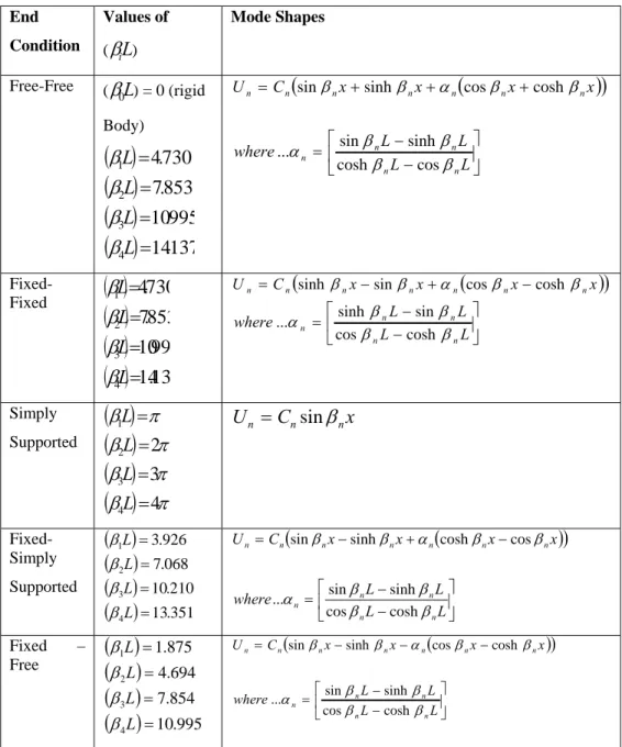
(25) 4 Beam Structure 4.1 Introduction Since beam is continuous structure, it can be modelled using three basics one dimensional element types are: (a) String element - for vibration in cables and wires, (b) Bar element- for transverse, (c) Beam element - for lateral vibration This formula being used to calculate the natural frequency developed from equation of motion of the beam. It has stated below. ω n = (β n L )2. c L2. (4.1). Where (β i L ) and table below 4.1 can be used to verify β n L , constant value. c=. EI ρA. (4.2. Where c is a constant value, E is Young modulus ( N / m 2 ) , I is the second moment of area (m 4 ) , ρ is the density (kg / m 3 ) , A is the cross-section area (m 2 ) , ω n is the natural frequency of vibration (rad/sec), L is the length of the beam, i represents number of frequencies and β n is determined from boundary conditions at the two ends of the beam. The beam simply supported from one end and fixed on the other end. These boundary conditions with the relevant values of β n L and mode shapes shown in below table 4.1. 23.

(26) Table 4.1: Angular frequencies and mode shapes for a beam in transversal vibration End. Values of. Condition. ( βiL). Free-Free. ( β0L) = 0 (rigid Body). (β1L) = 4.730 (β2L) = 7.853 (β3L) =10.995 (β4L) =14.137 FixedFixed. Simply Supported. FixedSimply Supported. Fixed Free. –. Mode Shapes. U n = C n (sin β n x + sinh β n x + α n (cos β n x + cosh β n x )) ⎡ sin β n L − sinh β n L ⎤ where ...α n = ⎢ ⎥ ⎣ cosh β n L − cos β n L ⎦. (β1L) =4.730 (β2L) =7.853 (β3L) =10.99 (β4L) =14.13 (β1L) =π (β2L) = 2π (β3L) = 3π (β4L) = 4π. U n = C n (sinh β n x − sin β n x + α n (cos β n x − cosh β n x )). (β1L) = 3.926 (β2 L) = 7.068 (β3L) = 10.210 (β4 L) = 13.351. U n = C n (sin β n x − sinh β n x + α n (cosh β n x − cos β n x )). (β1L) = 1.875 (β2 L) = 4.694 (β3 L) = 7.854 (β4 L) = 10.995. U n = C n (sin β n x − sinh β n x − α n (cos β n x − cosh β n x )). ⎡ sinh β n L − sin β n L ⎤ where ...α n = ⎢ ⎥ ⎣ cos β n L − cosh β n L ⎦. U n = Cn sin β n x. ⎡ sin β n L − sinh β n L ⎤ where ...α n = ⎢ ⎥ ⎣ cos β n L − cosh β n L ⎦. ⎡ sin β n L − sinh β n L ⎤ where ...α n = ⎢ ⎥ ⎣ cos β n L − cosh β n L ⎦. 24.

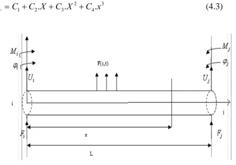
(27) 4.2 Finite Element Method Calculations Consider the beam as uniform beam element as shown in figure 4.1, the nodes i and j are located at the two beams end. The element is subjected to a transverse force distribution F, which is function of time and location. Each node has two degree of freedom, translation in the y-direction, u y and rotation φ . The nodal degree of freedom at nodes I are denoted as U I and φi and those at node j as U j and φ j . Whilst the external forces acting at node I are FI and M I (bending moment) and those acting at node j are FJ and M J . The element has a Young’s modulus E, a uniform crosssection area A, a moment of inertia I and density ρ . It is assumed that the transverse displacement variation in the x-direction is cubic, i.e., u y = C1 + C2 . X + C3 . X 2 + C4 .x 3. (4.3). Figure 4.1 Beam Element Configurations. Where the constant C1 , C2 , C3 and C4 are in general function of time and can be determined from the boundary conditions. The boundary conditions in general forms are:. 25.

(28) x = 0 ⇒ u x = ui , φ =. ∂u y ∂x. = φi. (4.4) x = L ⇒ uy = u j , φ =. ∂u y ∂x. = φj. Equation (4.1) should satisfy the conditions in equation (4.2) so that C1 and C2 can be found as C1 = U I C2 = φ I 1 (− 3U I − 2φI L + 3U J − φJ L ) L2 1 C4 = 3 (2U I + φI L − 2U J + φJ L ) L C3 =. (4.5). Substituting equation (4.3) into equation (4.1), the below is obtained which equation (4.4) ⎛ 3x2 2x3 ⎞ ⎛ 2x2 x3 ⎞ ⎛ 3x2 2x3 ⎞ ⎛ x2 x3 ⎞ + 2 ⎟⎟φi + ⎜⎜ 2 − 3 ⎟⎟U j + ⎜⎜ − + 2 ⎟⎟φ j uy = ⎜⎜1 − 2 + 3 ⎟⎟Ui + ⎜⎜ x − L ⎠ L L⎠ ⎝L L ⎠ ⎝ L ⎝ ⎝ L L⎠ (4.6). Or U y = N iU i + N 'iφi + N jU j + N 'jφ j. Where N i , N i' , N j , N 'j are the shape functions.. 26.

(29) 3x 2 2 x3 Ni = 1 − 2 + 3 L L 2 2x x3 N i' = x − + 2 L L 2 3 3x 2x Nj = 2 − 3 L L 2 x x3 N 'j = − + 2 L L. (4.7). The shape functions are shown in figure. 2 below. Figure 4.2: Shape function of a beam element The kinetics energy, T of the beam is obtained as: L. T =. 1 ' 2 ρ Vy dx 2 ∫0. (4.8). 27.

(30) Where ρ ' is the mass per unit length and Vy is the velocity in the ydirection. Substituting by ρ ' = ρA and Vy =. ∂u y ∂t. , into equation (4.6), gives. l ⎡ ∂u y ⎤ 1 T = ∫ ρA⎢ ⎥ .dx 2 0 ⎣ ∂x ⎦ 2. (4.9). Substituting equation (4.4) into equation (4.7), yields 2. L ⎡⎛ 3 x 2 2 x 3 ⎞ ⎛ ⎛ 3x 2 2 x3 ⎞ ⎛ x 2 x3 ⎞ ⎤ 1 2 x 2 x3 ⎞ + 2 ⎟⎟φi + ⎜⎜ 2 − 3 ⎟⎟U j + ⎜⎜ − + 3 ⎟⎟φ j ⎥ dx T = ∫ ρA⎢⎜⎜1 − 2 + 3 ⎟⎟U j + ⎜⎜ x − L L ⎠ L L ⎠ L ⎠ 2 0 ⎣⎝ ⎝ ⎝ L ⎝ L L ⎠ ⎦. (4.10) Where .. Ui =. ∂U i , ∂t. ∂φi , ∂t . ∂U j , Uj = ∂dt . ∂φ φj = j ∂t .. φ=. (4.11). Integrating equation (4.9), and writing in matrix form, gives: T=. 1 {U }T [m].{U } 2. (4.12). ⎧.⎫ where the superscript T indicates the transpose. The velocity vector, ⎨U ⎬ , ⎩ ⎭ is given by:. 28.

(31) ⎧ . ⎫ ⎪U i ⎪ ⎪. ⎪ φ . ⎧ ⎫ ⎪⎪ i ⎪⎪ ⎨U ⎬ = ⎨ . ⎬ ⎩ ⎭ ⎪U j ⎪ ⎪. ⎪ ⎪φ j ⎪ ⎪⎩ ⎪⎭. (4.13). And the mass matrix [m] is given by: 22 L 54 − 13L ⎤ ⎡ 156 ⎢ 22 L 4 L2 13L − 3L2 ⎥⎥ ρAL ⎢ [m] = 13L 156 − 22 L ⎥ 420 ⎢ 54 ⎢ 2 2 ⎥ ⎣− 13L − 3L 22 L 4 L ⎦. (4.14). Using the Euler-Bernoulli beam theory, the strain energy of the beam element can be expressed as: L ⎛ ∂ 2U Y 1 W ∫ EI ⎜⎜ 2 0 ⎝ ∂x 2. 2. ⎞ ⎟⎟ .dx ⎠. (4.15). Differentiating equation (4.4) with respect to x, substituting into equation (4.13), carrying the integration and writing in matrix form, yield. W =. 1 {U }T [k ].{U } 2. (4.16). Where the displacement vector, {U }, is given by:. 29.

(32) ⎧U i ⎫ ⎪φ ⎪ {∪} = ⎪⎨Ui ⎪⎬ ⎪ j⎪ ⎪φ j ⎪ ⎩ ⎭. (4.17). And the stiffness matrix [k] is calculated as: 6 L − 12 6 L ⎤ ⎡ 12 ⎢ 6 L 4 L2 − 6 L 2 L2 ⎥ ⎥. EI [k ] = ⎢ ⎢− 12 − 6 L 12 − 6 L ⎥ L3 ⎢ 2 2 ⎥ ⎣ 6L 2L − 6L 4L ⎦ The equation of motion is derived using Netwon’s second law and is defined as:. ([k ] − ω [m]){Um} = 0 2. (4.18). The mass and stiffness matrices increases along with increasing element of the beam and more nodes and more degree of freedom will be involved.. 30.

(33) 5 Experimental Work 5.1 Introduction The experimental work was carried at University of Surrey, Dynamics Research Laboratory. The dynamic test was conducted using an intact FRP composite beam with different boundary conditions. The main aim of this experimental work is investigate the modal parameters (frequency, mode shapes and modal damping) of the FRP composite beam. This test beam was supplied by STRONGWELL Company and the manual (contain both mechanical and physical properties) provided by the same company being used during the course of this research. 5.1.1. Measurement Preparations. This is done to ensure that the measurement will be as satisfactory as it can, pre-preparation are very important. How well the pre-preparation done will definitely determine the betterment of the expected data in our experiment. These are significance checks that have been done: 5.1.2. Identification of experimental model Excitation method The marked point on the beam sample Measuring method Hammer excitation force transducer Selection of the excitation signal Identification of Experimental Model. This is done by identifying the experimental model as prototype of footbridge (Footbridge Bridge). Since, it has been constructed with FRP (Fibre Reinforced Polymer) composite beam and set up as below in Figure 5.1. 31.

(34) Figure 5.1: Measurement FRP Beam 5.1.3. Position of the Accelerometer on the Beam. It is very mandatory to know position at which the accelerometer will be placed. This will be done in order to know the position where to put the reference and moveable accelerometer during the experiment measurement. We will use two different accelerometers and the detail will be explained in next chapter. We have 9 different point where accelerometer being positioned during the experiment. The distance between each point is relatively the same. 1. 2. 3. 4. 5. 6. 7. 8. 9. Figure 5.2: Point of the accelerometer 5.1.4. Point of Excitation. It is determine by dividing the model beam into 9 different points. Some mark has been placed on the FRP composite to indicate these points. The point of excitation decided on by using residual knowledge on dynamic test, therefore the excitation point is considered as point 3.. 32.

(35) 1. 2. 3. 4. 5. 6. 7. 8. 9. Figure 5.3: Point of Excitation at point 3. 5.2 FRP Composite Beam Test Descriptions In this research work, fibre reinforced polymer (FRP) beams were used as the test specimens. The dimensions of fibre reinforced polymer beams with 100 mm length, width 5 mm, thickness 3 mm. the FRP beam has the following properties cross-section area of 0.564e-3 m 2 , young modulus 17.926e9 N / m 2 , density 1827 Kg / m3 and poison ratio 0.3. Figure 5.4 shows the cross sectional details of the test beams.. Figure 5.4: Details of cross-section of the test beam The length of the beam is about 0.82 with different 9 point as described in chapter 5, distance between each point on the beam is equivalent 1.025e −1 m. two different accelerometer were used during the experiment, one being used as reference while other used moveable. The connection cable pointed toward y, z–direction to the Signal analyzer of the each accelerometers that is all response measurement was toward vertical direction. The impulses are used to excite different point on FRP composite beam to get response for different boundary conditions as indicated.. 33.

(36) For each case the response will plot in order to see the behaviour i.e. modal analysis behaviour of the FRP composite beam. All the vibration data acquired are imported to SPICE to process to acquired modal parameters are frequencies, damping ratio and mode shapes. We have two different technique in SPICE, Stochastic subspace identification technique and peakpicking technique. These methods are being used to process the acquired data, the sampling frequency, 3000Hz. These acquisition data were collected in Time-Domain and its being process with Stochastic Subspace identification The modal parameters (eigenfrequncies and mode shapes only) are extracted first using frequency-domain i.e., peak-picking technique, in order to give a quick look at the dynamic performance of the beam. Then the modal parameters of the beam i.e., natural frequencies, damping ratios and mode shapes are extracted from the measured data using time-domain technique i.e. the stochastic subspace identification technique, with sampling frequency 3000 Hz. The stochastic method works directly with the recorded time signals and it is based on linear calculations therefore it is considered to be more robust and faster than other methods. The experimental set-up is illustrated in figure 5.5.. Figure 5.5: The Experimental Set-up. 34.

(37) 5.3 Measurement Equipment The equipment was supplied by School of Engineering, University of Surrey, England. (1). Data Acquisition system. (2). Accelerometer. (3). Impact hammer. (4). Steel support. (5). PC with Software. 5.3.1. Data acquisition system. Phaser Analyzer (FFT analyzer), figure 5.6 was used as data acquisition system and has 4 input channels. Figure 5.6: Phaser (FFT) analyzer. 35.

(38) 5.3.2. Accelerometer. The accelerometer (Shear accelerometer) is of type 356B07 PCB Piezotronics CUBE ACCELEROMETER, figure 5.7 and measures the accelerometer of the vibrations. They are ICP tri-axial accelerometer with the following calibration values for reference accelerometer at y-axis, sensitivity 95.6 mV/g (9.75 mV / m / s 2 ), output bias 11.1 VDC, discharge time constant 0.3 seconds, transverse sensitivity 3.4 % while the z-axis sensitivity 96.9 mV/g (9.88 mV / m / s 2 ), output bias 11.3 VDC, discharge time constant 0.3 seconds, transverse sensitivity 3.0 %. Figure 5.7: Accelerometer 5.3.3. Impact Hammer. The impact hammer is of type figure 5.8 and used to determine component or system response to impacts of varying amplitude and duration. The impact has Sensitivity: (±15%) 1 mV/lbf (0.23 mV/N), Measurement Range: ±5000 lbf pk (±22000 N pk), Hammer Mass: 0.32 kg, Tip Diameter: 0.63 cm, Hammer Length: 22.7 cm, Head Diameter: 2.5 cm.. 36.

(39) Figure 5.9: Impact Hammer 5.3.4. Steel Support. The steel support, see figure 5.10 with 0.25m height, the length is 0.12m and the breadth 0.09m. These support used at both edges used to impose boundary conditions on the beam except free-free. The two support sides have bolts and nuts at the screw thread area.. Figure 5.10: Steel Support. 37.

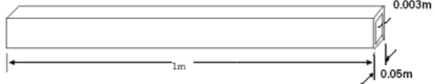
(40) 5.3.5. PC with Software. When measuring, the software Dactron (the real-time professional) was used. SPICE was software that was used for data analyzing and verification. 5.4 Experimental Specifications The specified apparatus is based around a Glass Fibre Reinforced Composite (FRP) square section describe in previous section. The dimension of the beam are conveyed in figure 5.11. Figure 5.11: Geometry of GFRP Composite beam In reality, the beam is 1000mm in length, however once it been clamped, the length between the ends become 820mm, as depicted in figure 5.12. 38.

(41) Figure 5.12: Beam position on fixed-fixed position The beam will be clamped in the apparatus as figure 5.12. figure 5.13 is a more detailed view of an end of the apparatus which allows the end conditions to be changed between simply supported and fixed, thus altering the boundary condition to which it is subjected to. This is achieved by adjusting the bolts which can be seen on the top of the apparatus.. Figure 5.13: End Condition Adjustment. 39.

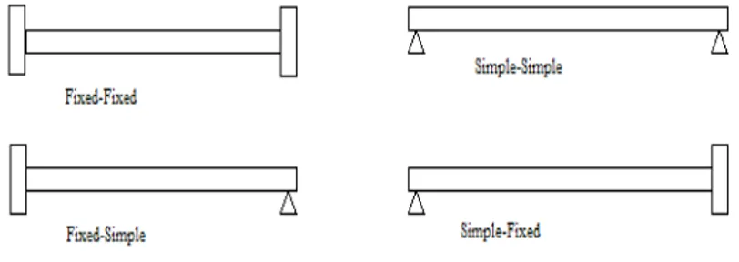
(42) The experimental apparatus will allow the beam will be clamped in four different boundary conditions as shown figure 5.14.. Figure 5.14: Boundary Conditions By considering a number of boundary conditions, it will be possible to observe how the beam behaves when excited and how the vertical displacement is affected. The natural frequencies will be monitored and the manner in which they differ between boundary condition will need to be considered.. 5.5 Experimental Results and Discussion This section presents the results from experimental investigation, where dynamic test with different boundary conditions were carried out. However, only output data from modal testing namely the mode shapes, frequencies were used to compare the analytical results. 5.5.1. Results. The dynamic test was carried out in laboratory with four different boundary conditions. The measured modal parameters are served as a reference for further comparison with analytical solution agreement. Using ANSYS software, an initial finite element model containing 9 elements is constructed using beam4 element type. The beam supports are simulated as three translation and rotational stiffness from each side using damper element. Only the first three bending modes are considered in the vertical direction. The sensitivity matrix of the stiffness supports in the FE model is. 40.

(43) calculated. In tables 5.1 and 5.2, the measured natural frequencies for the first three bending modes are given and compared to the finite element model. Table 5.1 Eigenfrequencies (Hz) of fixed-fixed boundary conditions Mode FRP Beam. 1. 2. 3. Measured. 241.318. 638.778. 950.979. Analytical. 318.79. 879.24. 17010.91. % Difference. 24.33. 27.35. 94.40. Figure 5.15 First bending moment. 41.

(44) Figure 5.16 Second bending moment. Figure 5.17: Third bending moment. 42.

(45) Table 5.2 Eigenfrequencies (Hz) of Fixed- free Boundary Conditions. FRP Beam. Mode. 1. 2. 3. Measured. N/A. N/A. N/A. Analytical. 50.0952. 313.964. 879.466. % Difference. Table 5.3 Eigenfrequencies (Hz) of Fixed-Simple Boundary conditions Mode FRP Beam. 1. 2. 3. Measured. 187.606. 670.906. 891.746. Analytical. 219.75. 712.25. 14668.60. % Difference. 14.63. 5.80. 93.92. Figure.5.18: First bending moment. 43.

(46) Figure 5.19: Second bending moment. Figure 5.20: Third bending moment. 44.

(47) Table 5.4: Eigenfrequencies (Hz) of Simple-Simple Boundary conditions. FRP Beam. Mode. 1. 2. 3. Measured. 132.660. 420.746. 870.00. Analytical. 140.71. 562.86. 1266.427. % Difference. 5.72. 25.25. 31.30. Figure 5.21: First bending moment. 45.

(48) Figure 5.22: Second bending moment. Figure 5.21: Third bending moment. 46.

(49) 6 Modelling in ANSYS 6.1 Introduction The finite element simulation was done by FEA package known as ANSYS. The FEA software package offerings include time-tested, industry-leading applications for structural, thermal, mechanical, computational fluid dynamics, and electromagnetic analyses, as well as solutions for transient impact analysis. ANSYS software solves for the combined effects of multiple forces, accurately modelling combined behaviours resulting from "multiphysics" interactions. This is used to perform the modelling of the beam and calculation of natural frequencies with relevant mode shapes.This is used to simulate both the linear & nonlinear effects of structural models in a static or dynamic environment. Advanced nonlinear structural analysis includes large strain, numerous nonlinear material models, nonlinear buckling, post-buckling, and general contact. Also includes the ANSYS Parametric Design Language (APDL) for building and controlling user-defined parametric and customized models. The purpose of the finite element package was utilised to model the Fibre reinforced polymer (FRP) beam in 3-D as SHELL93 (8node93). This package enables the user to investigate the physical and mechanical behaviour of the beam. The FE-model parameters extracted from the Strongwell manual [19] provided with the composite beam specimen. The FE-model constructed along vertical direction only which made it applicable to the real bridge model. The load applied from pedestrian used to come in vertical directions during the walking or movement along the bridge that is why the analysis is being done toward vertical directions. Though, the specimen has anisotropy properties but we have only considering the vertical direction that is why the linear isotropic parameter only used.. 47.

(50) 6.2 Procedure in Modelling ANSYS There are major and sub important steps in ANSYS model, pre-processing, solution stage and post-processing stage.. Figure 6.1: FE-Analysis Steps 6.2.1. Requirement Specification. This step is done in pre-processing in ANSYS. In this work the beam element model used know was SHELL93 and it was specification at the. 48.

(51) pre-processing stage. The SHELL93 element is applicable to this model for the structural meshing and boundary condition applications. Table 6.1:Input data for Modelling of the beam Geometry Definition. Values. Thickness. 3e-3m. Young modulus. 17.926e9. Density. 1827. Width. 0.05m. Length of the beam. 0.82m. Poisson Ratio. 0.3. The parameter specified in the table above indicated that only vertical direction analysis was carried on the beam. This is also applicable to the modal analysis experiment in the previous section. 6.2.2. Idealization Specification. This is sub-stepping procedure in model context represents a 3D shell definition. This model is optimized for rapid FEM analysis and is composed of 2D geometry, beam surface model. It is easy to locate and calculate the numerical position in shell geometry; beam shell model can be defined of the 3D definition. The analysis type is defined as modal 6.2.3. Mesh Generation. The generation of a mesh on the idealized geometry is done through meshed model. The meshing depend on the configuration for the model, the general rules are carried out by setting a density for the mesh. In this application, loads and boundary conditions are added in the input file. The solver input file consists of mesh elements, nodes and load cases. The input file is generated from the application containing mesh elements, nodes and boundary conditions are added to the file.. 49.

(52) 6.2.4. Analysis. This is a stage where solution was conducted. It was the step to preprocessing and different stages of analysis took place. The load is applied to edges of beam, this was easier to implement in SHELL model. And the other entire complex algorithm in FEM solved.. 6.2.5. Post-processing. At this stage the results of analysis are obtained numerically and graphically.. 6.3 ANSYS Graphical Results These are following dynamic analysis for different boundary conditions. The result obtained are generated inform of graphical view which show the modal concept and influence of each boundary conditions for the vertical frequencies of the FE shell model of the beam. 6.3.1. Simple-Simple Boundary Condition. The results shown below are the graphical solution of deformed and undeformed shape for first 2 modes.. 50.

(53) Figure 6.2: Mode 1 under simple-simple boundary conditions. Figure 6.3: Mode 2 under simple-simple boundary conditions. 51.

(54) Table 6.2: the table shows the mode frequencies in Hz predicted theory and ANSYS. 6.3.2. Mode. Theory. ANSYS. Percent Error. 1. 140.710. 199.790. 29.55. 2. 562.860. 532.007. 5.50. Fixed-Fixed Boundary Condition. The results shown below are the graphical solution of deformed and undeformed shape for first 2 modes.. Figure 6.4: Mode 1 under fixed-fixed boundary conditions. 52.

(55) Figure 6.5: Mode 2 under fixed-fixed boundary conditions. Table 6.3: the table shown the mode frequencies in Hz predicted theory and ANSYS. 6.3.3. Mode Theory. ANSYS. Percent Error. 1. 318.890. 327.671. 2.70. 2. 878.240. 813.552. 7.42. Fixed-Simple Boundary Condition. The results shown below are the graphical solution of deformed and undeformed shape for first 2 modes. 53.

(56) Figure 6.6: Mode 1 under fixed-simple boundary conditions. Figure 6.7: Mode 2 under fixed-simple boundary conditions. 54.

(57) Table 6.4: the table shown the mode frequencies in Hz predicted theory and ANSYS. 6.3.4. Mode Theory. ANSYS. Percent Error. 1. 219.750. 233.851. 6.08. 2. 711.250. 745.298. 4.49. Fixed-Free Boundary Condition. The results shown below are the graphical solution of deformed shape for first 2 modes. Figure 6.8: Mode 1 under fixed-free boundary conditions. 55.

(58) Figure 6.9: Mode 2 under fixed-free boundary conditions Table 6.5: the table shown the mode frequencies in Hz predicted theory and ANSYS Mode Theory. ANSYS. Percent Error. 1. 50.0952. 51.704. 1.45. 2. 313.964. 307.094. 2.19. The ANSYS results also show small relative errors compared with the analytical solution as shown in table 6.2, 6.3, 6.4 and 6.5.. 56.

(59) 7 Discussion 7.1 Introduction With the completion of experimental, analytical and ANSYS section of this research work, it is now possible to analyse result found in chapter 5 of this work. This section will focus on the findings of the studys, the comparisons which can be made between the different methods, and most importantly, the effect that frequency has on the FRP composite beam.. 7.2 Comparison of Method Four different area of analysis was conducted on the beam, analytical method, finite element methods (1 and 2 elements), Experimental study, ANSYS Model. Different observations were made in this work from previous sections. It is mandatory to mention the density values used within the calculations and ANSYS study. This manual provided with the composite beam specimen was used in the experiment, the density was quoted as having a value ρ = 1716 − 1937kg / m 3 . there are different density values considered when determining the natural frequencies using analytical and finite element methods and ANSYS. The mean average of the maximum and minimum density values was taken and found to be ρ = 1827kg / m 3 . these three density values adequately covered the density range provided. When comparing natural frequencies calculated using different methods and the three density values, it can be seen that although the natural frequencies obviously vary, the spread of the results is fairly small (due to the small density change). It was noticed that the value of ρ = 1827kg / m 3 best suitable the experimental results and it was decided to use this density values in all the comparisons in the every part of this work. Reference to the appendix 3, when comparing analytical method to the finite element with 1 element, it can be seen that although the values. 57.

(60) obtained for the natural frequencies are in a similar, there are some issues with inaccuracy. This is because finite element method is an approximate solution which is intended to be use when analytical solution is difficult to obtain. Significant improvement may be seen when the number of elements considered is increased from one to two in Appendix 4. by comparing results and calculating the relative errors between the analytical method and the finite method at the first natural frequency, table 7.1 below was constructed. Table 7.1: % Error between FEM & Analytical Solution for Mode 1 Boundary Condition. Finite Element Method-1. Finite Element Method-2. Element (Percent error). Element (Percent error). Fixed-Fixed. N/A. 1.76. Simple-Simple. 9.945. 0.33. Fixed-Simple. 24.82. 0.96. Fixed-Free. N/A. N/A. From the table above, it can be seen that the relative errors between the finite element method and the analytical solution are significant reduced when the number of elements is increased, there will be a greater number of nodes in the structure which means that a better idea of the displacement and deformation of the structure can be found. This will lead to mode shapes of the system becoming more similar to the analytical mode shape. In a similar manner, the ANSYS results also show small relative errors with the analytical solution as found in table 6.2, 6.3, 6.4 and 6.5. When considering the natural frequency, further observation about the errors between these methods may be made. The increase in number of elements reducues the errors. By referring to mode shapes provided from ANSYS in chapter 6 of this work, it can be seen that a relatively smooth curves is produce with increase in number of elements. Some observations were also made in experimental results as indicated in figure 5.15 – 5.21, the natural frequency may be determined by the peak on the Frequency-Amplitude graphs. In theory, the maximum displacement of the beam should be at the point 5 (that is the centre of the beam) and in. 58.

(61) most cases this has been achieved. If this is not case then either point 4 or point 6, just off the centre line of the beam has had the maximum displacement. From the result in table 5.1 – 5.4, there are discrepancy with the first natural frequency recorded during the experimental study to that of the analytical solution, finite element and ANSYS. Initially it was thought that it was partially due to the fact the density value of the beam was different to that used in the calculation but it was then decided that since the density does not vary to a great extent compared to the value of the natural frequency then this couldn’t be the case. A more likely cause of these discrepancies could be due the way that the boundary conditions are applied to the beam during the experiment. In the analytical, finite element and ANSYS methods, all boundary conditions are considered to be ideal, i.e perfectly for a fixed end and perfectly simply supported for a simply supported end. In experimental setup, a fixed end is achieved by combining two simply supported setup’s as shown in figure 7.1.. Figure 7.1: Experimental Fixed End The issue of increase in stiffness at the boundary to a single simply supported end, there will still be some movement at the end of the beam and will therefore not achieve the ideal fixed end condition. It would therefore be useful to design a method of producing a more effective fixed end for future experimental work. Also, clamping system on the apparatus was over-tightened when applying a simply supported condition to the beam. That means the beam a lot stiffer at the end which will result in the higher than natural frequencies.. 59.

(62) 7.3 Effect of Boundary Conditions on Natural frequency The observation made in table 5.1 to 5.4, the natural frequency is lower under simply supported condition than fixed conditions (except for experimental result which was explained in the previous section). This is due to the below equation:. ωn =. k m. (7.1). The fixed-fixed condition will generate greater stiffness than simply supported since the mass remain constant in the situation. The overall natural frequency is reduced under simply supported due to the reduced stiffness. But, fixed-fixed boundary condition is best applicable to the real bridge.. 60.

(63) 8 Conclusion In this section of the report, series of reasonable observations were made and discussed below. The dynamic investigation of a fibre reinforced polymer beam was carried out in this work. The modal analysis was performed to the natural frequencies and mode shapes. The fundamental vertical frequencies for four boundary conditions were estimated in experimental and analytical ways. When comparing the experimental results (frequencies, mode shapes etc) with analytical results, there are some discrepancies with the error between the two values. It was likely that this is connected with the manner in which boundary conditions are applied in the beams. It seems that the fixed boundary conditions allows for too much movement at the end and that simply supported end is much stiffer than would be experienced under the analytical solution. It is advisable to redesign the experimental apparatus to give better results with different boundary conditions. The finite element method results compared to the analytical solution, it can be observed that the accuracy of the finite element method increases as the number of the element is increased. It has been seen that when comparing the results of second mode from the finite element method with analytical solution, that a greater number of elements is required to adequately reproduce the more complex mode shapes Finally, there are fair agreements between experimental results and analytical which was the target of this research work. The reason for the discrepancies has been discussed in previous section.. 8.1 Future Work The work can be extended by apply to Structural Health Monitoring (SHM). We can apply this work in the case of damage detection techniques in NDT. The experimental work can also be improved by recording cross channel where displacement of the beam is measured as a function of the applied force.. 61.

(64) 9. References. 1.. Cadei, J., (2003) “The Nesscliffe Bypass Wilcot footbridge-atriumph of FRP”, Concrete, June 2003,pp.37. 2.. Firth, I., (2002) “New Materials for New Bridges-Halgavor Bridge, UK”, Structural Engineering International, n.2v 12.. 3.. Eric Johansen, et. al., (1996) “A Design and Construction of Two Pedestrian Bridges in Haleakala National Park, Maui, Hawaii,@ Proceedings, Fiberglass-Composite Bridges Seminar, 13th Annual Bridge Conference and Exhibition, Pittsburgh, PA, June 3.. 4.. Sieble, F.; et. al., (1994) "Seismic Retrofitting of Squat Circular Bridge Piers with Carbon Fiber Jackets," Report No. ACTT-94/04, November 1994, pp. 12-20, University of California at San Diego.. 5.. Piers with Carbon Fiber Jackets, Report No. ACTT-94/04, November 1994, pp. 12-20, University of California at San Diego.. 6.. Ballinger, C. A. (1990). “Structural FRP composites-Civil Engineering’s Material of the Future” Civil Engineering, ASCE, 60(7), pp. 63-65.. 7.. Nagraj, V., and Ganga, Rao, H. V. S. (1997). “Static Behavior of Pultruded GFRP Beams”, Journal of Composites for Construction, Vol. 1, No. 3, August, pp. 120-129.. 8.. Davalos, J. F., and Qiao, P. (1997). “Analytical and Experimental Study of Lateral and Distortional Buckling of FRP Wide-Flange Beams”, Journal of Composites for Construction, Vol. 1, No. 4, pp. 150-159.. 9.. Sotiropoulos, S. N., Gangarao, H. V. S., and Allison, R. W. (1994) “Structural Efficiency of Pultruded FRP Bolted and Adhesive Connections”, Proceedings of 49th Annual Conference, Composite Institute, The Society of Plastics Industry Inc., Cincinnati, Ohio, SPI/Composite Institute, New York, N.Y.. 10.. Barbero, E. J., Fu, S. H. and Raftoyiannis, I. (1991). “Ultimate Bending Strength of Composite Beams”, Journal of Materials in Civil Engineering, Vol. 3, No. 4, November, pp. 292-306.. 62.

(65) 11.. Bank L C,Mosallam A S,Gonsior H E (1990) “Beam-to-column connections for pultruded FRP structures[C]” Proceedings of the 1st Materials Engineering Congress .New York:ASCE,1990:804-813.. 12.. Sotiropoulus, GangaRao, and Barbero, “Static Response of Bridge Superstructires Made of Fiber Reinforced Plastic” Use of Composite Material in Transportation System American Society of Mechanical Engineers, Applied Mechanics Division, AMD, ASME: New York, NY, v129, 57-65.. 13.. R.Lopez-Anido and H.V.S GanagaRao, (1997) “Design and Construction of Composite Material Bridge,” US-Canada-Europe Workshop on Bridge Engineering, Zurich, Switzerland, July 14-15, 1997, 1-8.. 14.. Ballinger C.A, “Advancied Composite in the construction Industry,” Materials Working for You in the 21st Century, International SAMPE Symposium and Exhibition, SAMPE: Covia, CA, V37 (1992) 1-14.. 15.. Brailsford, S.M. Milkovich, D.W. Prine,J.M.Fildes, (1995) “Definition of Infrastructure Specific Market for Composite Materials” Tropical Report,'Northwestern University BIRL Project P93-121/A573, July 11, 1995.. 16.. Khan M.A.U (1999) “Non-destructive Testing Applications for Commercial Aircraft Maintenance” Proceeding of the 7th European Conference on Non-Destructive Testing, v.4, 1999.. 17.. Bar-Cohen Y. (199) “Emerging NDE Technologies and Challenges at the Beginning of 3rd Millennium” Material Evaluation, 1999.. 18.. ANSYS, Analysis Guide, ANSYS release 8.0, SAS IP In, Houston.. 19.. Strongwell Corporation, (2003), “Composite Fiberglass Building Panel System”, Composite bronchure.. 63.

(66) Appendix 1, Terminogoly Several definitions of the terminology critical to this study are contained within this section. Dynamic Force - a force that changes with respect to time (not static). Vibration - Oscillation of a system in alternately opposite directions from its position of equilibrium, when that equilibrium position has been disturbed. Two types are free vibration and forced vibration. Forced vibration takes place when a dynamic force disturbs equilibrium in the system. Free vibration takes place after the dynamic force becomes static (or zero). Amplitude - The offset of equilibrium of the system at a given time, also known as the magnitude of the wave when plotting displacement, velocity, or acceleration against time. Period- The amount of time it takes for one cycle. Cycle - A complete motion of a system starting at any given point of magnitude and direction that ends with the same magnitude and direction (i.e., the motion over a full period). Frequency- Number of cycles over a given time, usually cycles per second (also called Hz). Natural Frequency - a frequency at which the system will vibrate freely when excited by a sudden force. Fundamental Natural Frequency - The lowest natural frequency for the system at which a system will vibrate. Resonance - a condition where a system is excited at one of its natural frequencies. Damping - a property of energy dissipation within the system. More damping results in a quicker decay of amplitude in free vibration. When less damping is present, the system retains its energy for a longer amount of time.. 64.

(67) Fast Fourier Transform (FFT) - An algorithm for computing the fourier transform of a set of discrete data values. The FFT expresses the data in terms of its component frequencies. FFT Spectrum - The relative contribution of frequencies in a trace of amplitude over a time range. This is obtained by performing an FFT of the data. Mode shapes - The shape of a system showing displacements when undergoing vibration.. relative. Node - The point location on a mode shape that undergoes zero relative displacement.. 65.

(68) Appendix 2, Calculation for FEM for Natural frequencies of Beam (1 Element) 22 L ⎡ 156 ⎢ 4 L2 ρAL ⎢ 22 L Mass Matrix: [m] = 13L 420 ⎢ 54 ⎢ 2 ⎣− 13L − 3L. 54 − 13L ⎤ 13L − 3L2 ⎥⎥ 156 − 22 L ⎥ ⎥ − 22 L 4 L2 ⎦. 6 L − 12 6 L ⎤ ⎡ 12 ⎢ 6 L 4 L2 − 6 L 2 L2 ⎥ EI ⎥ Stiffness Matrix: [k ] = 3 ⎢ L ⎢− 12 − 6 L 12 − 6 L ⎥ ⎥ ⎢ 2 − 6 L 4 L2 ⎦ ⎣ 6L 2L Equation of Motion: ⎛ ⎡ 12 6L −12 6L ⎤ 54 13L ⎤ ⎞⎧Umi ⎫ ⎡ 156 22L ⎟⎪ ⎜ ⎢ ⎪ ⎢ 2 2 ⎥ 2 13L − 3L2 ⎥⎥ ⎟⎪φmi ⎪ ⎜ EI ⎢ 6L 4L − 6L 2L ⎥ 2 ρAL ⎢ 22L 4L ⎜ L3 ⎢−12 − 6L 12 − 6L⎥ − ω 420 ⎢ 54 13L 156 − 22L⎥ ⎟⎨Um ⎬ = 0 ⎟⎪ j ⎪ ⎜ ⎢ ⎢ 2 2 ⎥ 2 2 ⎥ ⎟⎪ ⎜ ⎣−13L − 3L − 22L 4L ⎦ ⎠⎩φmj ⎪⎭ ⎝ ⎣ 6L 2L − 6L 4L ⎦. Where: λ. ρAL4ω 2 420 EI. (Note: these calculations were completed using a density of ρ = 1827kg / m 3 . for calculations with different density values, this figure was substituted).. 66.

(69) Fixed-Fixed. Not possible for Single Element Simple-Simple ⎡4 L2 − 4 L2 λ ⎢ 2 2 ⎣ 2 L + 3L λ. (4 L. 2. 2 L2 + 3L2 λ ⎤ ⎧φmi ⎫ ⎬=0 ⎥⎨ 4 L2 − 4 L2 λ ⎦ ⎩φm j ⎭. − 4 L2 λ )(4 L2 − 4 L2 λ ) − (2 L2 + 3L2 λ )(2 L2 + 3L2 λ ) = 0. 12 L4 − 44 L4 λ + 7 L4 λ2 = 0 ⇒ 3.165λ2 − 19.89λ + 5.43 = 0 19.89 ± 19.89 2 − (4 × 3.165 × 5.43) =0 2 × 3.165 λ = 0.286 or λ =6 981.31 420 × 17.926 × 10 9 × 2.085 × 0.286 = 981.31rad / s ∴ f1 = 4 −4 2π 1827 × 5.64 × 10 × 0.82 f1 = 156.18Hz. ω1 =. 4496.95 420 × 17.926 × 10 9 × 2.085 × 6 = 4496.95rad / s ∴ f 2 = −4 4 2π 1827 × 5.64 × 10 × 0.82 f 2 = 715.7 Hz. ω2 =. 67.

No results found