Analysis of major flood events on Rio Grande - Bernard to San Marcial

f

[

f

I

r

r

I

l

I

[

ANALYSIS OF MAJOR FLOOD EVENTS

ON RIO GRANDE - BERNARDO TO SAN MARCIAL

:·I·

! : ' '

I:

II

'I:

·.1'

.,

ANALYSIS OF MAJOR FLOOD EVENTS

ON RIO GRANDE - BERNARDO TO SAN MARCIAL

Submitted to

u.s.

Army Corps of Engineers

Albuquerque District

Prepared by

Daryl B. Simons

Principal Engineer

Ruh-Ming Li

Principal Hydraulic Engineer

Yung Hai Chen

Associate Principal Engineer

George K. Cotton

Hydrologist

Simons, Li & Associates, Inc.

PO Box 1816

Fort Collins, Colorado 80522

Our Project Number:

NM-COE-02

I

I

I

I

I

I.

I

II.

I

I

_III.

I

I

IV.

I

I

v.

I

I

VI.

I

I

I

I

I

TABLE OF CONTENTS LIST OF TABLES • • LIST OF FIGURES INTRODUCTION 1.1 General • DATA SUMMARY • 2.1 Hydrology • • • • • 2.2 Hydraulics • • • • • • • •

2.3 Spatial and Temporal Design

2.4 Bed-Material Size •

2.5 Resistance to Flow

QUALITATIVE AND QUANTITATIVE ANALYSIS

3.1 Flood History from Rio Puerco and Rio Salado

3.2 Alluvial Deposits at the Tributaries SEDIMENT TRANSPORT • 4.1 General • • • • 4.2 4.3 4.4 4.5 4.6

Sediment Transport Capacity • Flow Conditions Determination Bed-Load Transport Capacity • • Suspended Load Transport Capacity •

Calibration • • • • • SEDIMENT SUPPLY

.

.

. . .

. . .

iv v 1 3 3 13 14 19 19 24 24 29 32 32 32 33 33 34 35 39 5. 1 General • • • • • • • • • • • • • • • • • • • 39

5.2 Sediment Rating Equations for Tributaries • • • • • • 39

SEDIMENT ROUTING • 6.1

6.2

General • • • • • • •

Case I: 50-Year Floods from Both Rio Puerco and

Rio Salado

6.3 Case II: 100-Year Floods from Both Rio Puerco and

6.4 6.5 6.6

6.7

Rio Salado

Case III: Standard Project Flood from Rio Puerco

and Rio Salado

Cases IV,

v,

and VI

Cases VII, VIII, and IX

Case X

.

.

.

.

. . .

.

.

i i 41 41 45 49 49 56 56 69

,I

I

I

I

I

'I

I

I

I

I

I

I

I

I

I

I

,I

I

:1

VII. REFERENCES • APPENDIX. A:

TABLE OF CONTENTS (Continued)

SAND WAVE CELERITY

iii

Page 69

I

I

LIST OF TABLES

I

Page

Table 2. 1 Floodway Velocities at 10,000 cfs

.

. . .

15

Table 6.1 Volume of Bed Material Sediment Reaching the

I

Floodplain Reaches

. . .

. .

. . .

.

43

Table 6.2 Aggradation/Degradation - Case I

.

. . .

.

46

I

Table 6.3 Aggradation/Degradation - Case II

. . .

.

50

Table 6.4 Aggradation/Degradation - Case III

.

53

I

Table 6.5 Aggradation/Degradation - Case IV

. . . .

.

57

Table 6.6 Aggradation/Degradation - Case

v

. .

58

Table 6.7 Aggradation/Degradation - Case VI 59

I

Table 6.8 Aggradation/Degradation - Case VII

.

.

. . .

63

Table 6.9 Aggradation/Degradation - Case VIII

.

. . .

.

64

I

I

Table 6.10 Aggradation/Degradation - Case IX

.

.

.

.

65

Table 6. 11 Comparison of Maximum Water-Surface Elevations

.

70

I

Table 6.12 Aggradation/Degradation, Case X

. .

.

.

. . . .

71

I

I

I

I

I

I

I

I

iv

I

I

LIST OF FIGURES

I

I

Figure 2. 1 Figure 2. 2 Case I: Case II: 50-year flood Rio Puerco and Rio Salado 100-year flood Rio Puerco and Rio 4

Salado • • 5

I

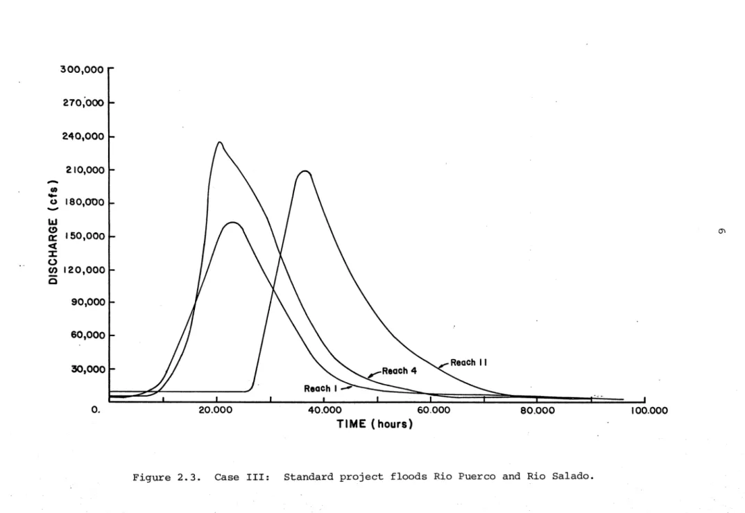
Figure 2.3 case III: Standard project floods Rio Puerco

and Rio Salado

. . .

.

.

. .

6

I

Figure 2.4 Case IV: 50-year flood Rio Puerco

.

7

Figure 2.5 Case V: 100-year flood Rio Puerco

.

.

8

Figure 2.6 Case VI: Standard project flood Rio Puerco 9

I

I

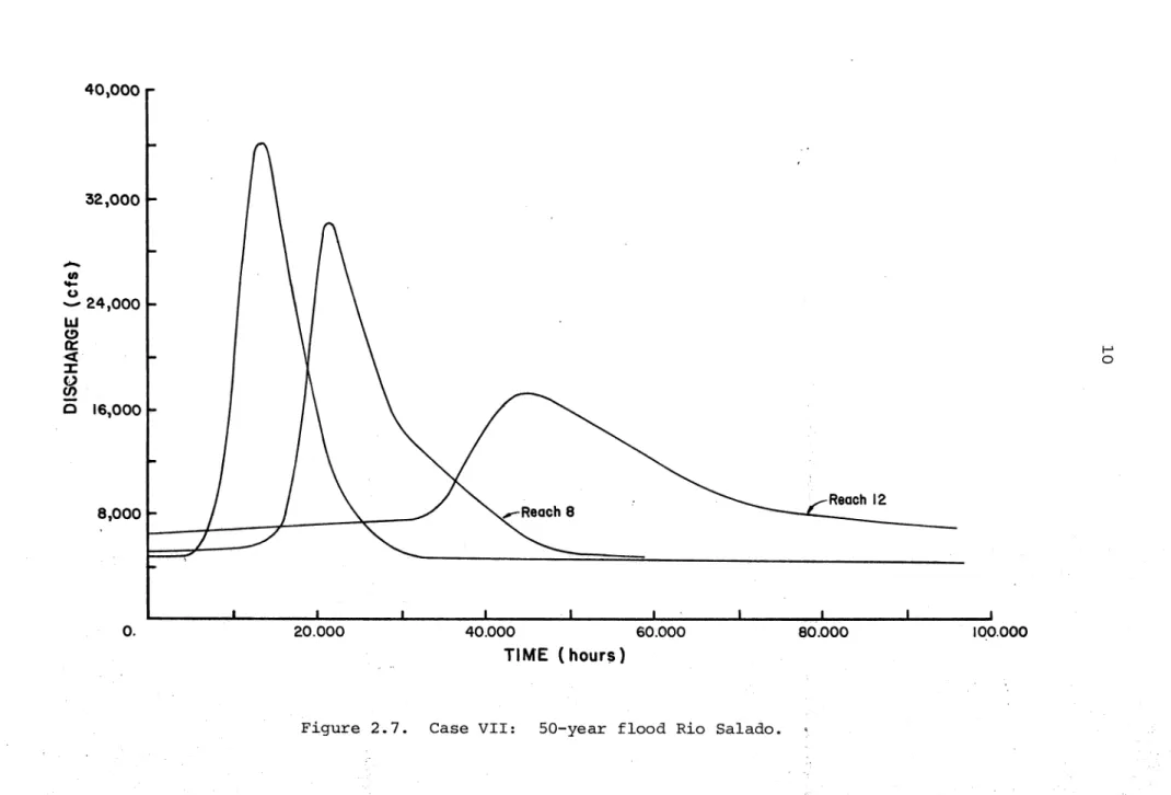
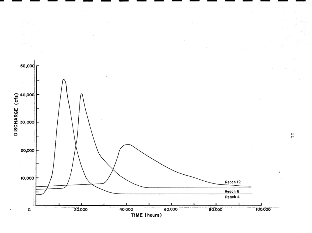
Figure 2.7 Case VII: 50-year flood Rio Salado 10

Figure 2.8 Case VIII: 100-year flood Rio Salado

. . .

11

I

Figure 2.9 Case IX: Standard project flood Rio Salado

. . . .

12

I

Figure 2.10 Index map of Rio Grande Figure 2.11 Superposition of hydrographs • • • • 17 18

I

Figure 2.12 Grain size distribution San Acacia and San

Marcial reaches • • • 20

Figure 2.13 Manning's n-value versus discharge Rio Grande

near Bernardo

. .

. . . .

.

. . .

. . .

. . . .

21

I

I

Figure 2. 14 Manning's n-value versus discharge Rio Grande San Acacia

.

.

.

.

. . .

.

.

.

.

. .

. . .

22

Figure 2.15 Manning's coefficient- Rio Grande floodway at

I

_{Figure 3.1} San Marcial _{Rio Grande Floodway near San Marcial} • • • • • • • • • • • • • • • 23 ₂₈

I

Figure 3.2 Photo of the Rio Grande taken at San Marcial

during the 1937 flood • • • • • • • • • • • • • 30

I

Figure 4.1 Correction factor as a function of velocity

for Bernardo reach

.

. . . .

. . .

. . .

37

Figure 4.2 Correction factor as a function of velocity

for San Acacia and San Marcial

. .

. .

.

. .

.

.

.

.

38

I

I

Figure 6.1 Aggradation at the Rio Puerco confluence- Case I 47

I

I

LIST OF FIGURES (continued)

Page

Figure 6.2 Aggradation at the Rio Salado confluence

-I

Case I

. . . .

. .

.

. . .

. . . .

.

. . . .

48

Figure 6.3 Aggradation at the Rio Puerco confluence

-I

Case I I

. .

.

.

.

. . .

.

. .

51

I

Figure 6.4 Aggradation at the Rio Salado confluence

-Case I I

.

.

. .

. . .

.

.

. . .

52

Figure 6.5 Aggradation at the Rio Puerco confluence

-Case III

. . .

.

.

.

. . .

.

. . .

54

I

Figure 6.6 Aggradation at the Rio Salado confluence

-Case III

. . .

.

.

.

. . .

55

I

Figure 6.7 Aggradation at the Rio Puerco confluence

-Case IV

. . .

. . .

. . .

60

I

Figure 6.8 Aggradation at the Rio Puerco confluence

-Case V

. .

.

.

.

.

.

. . .

.

. . .

. .

61

I

Figure 6.9 Aggradation at the Rio Puerco confluence

-Case VI

. .

. . .

.

.

. . .

. .

62

I

Figure 6.10 Aggradation at the Rio Salado confluence

-I

_{Figure 6. 11} .case VII _{Aggradation at the Rio Salado confluence}

.

. .

. . .

. . .

_-

. . .

66

Case VIII

.

.

.

. .

. . .

.

. .

.

.

.

.

67

Figure 6.12 Aggradation at the Rio Salado confluence

-I

Case IX

.

. .

. . .

.

.

.

. . . .

68

I

I

I

I

I

I

I

vi

I

I

I

I

I

I

I

I

I

I

I

I

I

I

I

I

I

I

I

I. INTRODUCTION 1.1 General

Presented in this report is the hydraulic and geomorphic analysis of the Rio Grande from Bernardo to San Marcial, New Mexico, for major flood events

from the Rio Puerco and Rio Salado tributaries. The study system on the Rio

Grande includes approximately 61 miles of the floodway. The major flood

events studied are the 50-year, 100-year and standard project floods from the

Rio Puerco and Rio Salado watersheds. These two tributaries are heavy

contri-butors to the sediment problem in the main stem, especially during floods. A

separate analysis of these floods was developed to supplement the evaluation

of the long-term response of the Rio Grande. Previous study by Simons, Li &

Associates has evaluated the long-term response of the Rio Grande for various

alternatives of development on the Rio Puerco and Rio Salado watersheds. This

report will provide a more detailed analysis with a finer spatial and temporal resolution as required for short-duration floods.

A three-level approach is conducted to delineate the potential

sedimen-tation problems in the main stem of the Rio Grande resulting from major

floods. A qualitative study of previous floods from the Rio Puerco and Rio

Salado tributaries is conducted based on historical records and photographs. A quantitative study of the nature of deposition at the Rio Puerco and Rio Salado tributaries and in the main stem of the Rio Grande is conducted based on the bed-load regression equations, equilibrium concepts, and alluvial fan

morphology. The third level applies a known-discharge sediment routing model

to evalaute the conditions for the study system. The mathematical model

developed by Simons an? Li for routing sediment by size fractions is used to estimate the general scour and deposition in the study system as a function of

time and discharge. This model uses hydraulic conditions. determined by the

u.s.

Army Corps of Engineers HEC-2 program. The model extends the

conven-tional HEC-2 analysis by recognizing that the channel bed is movable. The

channel geometry is adjusted to simulate the response to scour and deposition

within reaches of the study system. The sediment transport relationships in

this report are consistent with the regression equations for sediment

transport developed previously in this study. The actual relationships are

the Meyer-Peter, Muller bed-load equation and the Einstein suspended bed-load equation which have been calibrated based on known data.

2

Use of the more complex sediment routing model provides a finer :t:esolu-tion of the aggrada:t:esolu-tion/degrada:t:esolu-tion response due to major storms from the Rio

Puerco and Rio Salado tributaries. The effects of these events are quite

significant and will affect long-term conditions in the mainstem. The

deposi-tional character of these tributaries is determined within limits consistant with present state of the art sediment transport technology and consistant with the strong role they play in the hydraulic conditions and sediment

transport of the Rio Grande system below Bernardo.

'1;· .

. ~ . ; ~

~.1'

. .

:1!.

' . ' '

'1:

. .

I

·11

! .-! !

I

I

I

I

I

I

I

I

3

II. DATA SUMMARY

The comprehensive analysis of the alluvial system of the Rio Grande

requires a good data base for all levels of analysis. The important data

needed for this portion of the study can be grouped into the following

categories: hydrology, hydraulics, channel geometry, bed-material size,

resistance to flow, sediment transport, and topographic information. This

data base has been developed in previous reports in this study (see

"Preliminary Evaluation of River Response of the Rio Grande from Bernardo to

Elephant Butte Dam," Simons, Li & Associates, May 8, 1981). The specific

application of this data base to the problem of sedimentation from major

floods is discussed in this chapter. The sediment transport theory and

calibration methods for the mathematical models are presented in a separate chapter.

2. 1 Hydrology

I

The flood hydrographs used in this study include the 50-year, 100-year

and standard project floods as reported by the Albuquerque District of the

I

I

I

I

I

I

I

I

I

I

u.s.

Army Corps of Engineers in 1979 for the Rio Puerco and Rio Salado. Nine cases of flooding from these two tributaries were developed flooding on the main stem. 1. 2. 3. 4. 5. 6. 7. 8. 9.

The following cases were analyzed:

50-year floods from both Rio Puerco and Rio Salado 100-year flood from both Rio Puerco and Rio Salado

Standard project floods from both Rio Puerco and Rio Salado 50-year flood from Rio Puerco

100-year flood from Rio Puerco

Standard project flood from Rio Puerco 50-year flood from Rio Salado

100-year flood from Rio Salado

Standard project flood from Rio Salado

A constant inflow of 5000 cfs from Bernardo was assumed for all cases. The discharges at various points along the mainstem were established using a

full dynamic method of routing water. Results of this routing are shown in

Figures 2.1 to 2.9 at selected river miles. The results show the very

signi-ficant peak discharge attenuation and distortion of the flow from the tribu-taries as they move along the mainstem of the Rio Grande (see page 17 for

-

Cl)

....

( )

-40,000 32,000 LL1 24,000 (!) 0: <l :I: 0

en

c

16,000 8,000

1----f+---..o/

-·o.

20.000

40.ooo

·so.ooo

80.000

TrME

(hours)

Figure 2 .1. Case I: SO~year flood Rio Puerco and Rio Salado.

H::-Reach I) Reach 4

100.000

----~-~---

'--so,ooJ

I

_: i

I

I

48,009 -_II) 1 _! - I

~

I

LL1 j (!) 1 a: 36,000 <[ ~ 0

en

2i

24,ood

12,000' 0.

i

lJ1 '-Reach I 40.000 Tl ME (hours)

300,000 27o:ooo 2,..0,000 210,000

-

....

en u 1ao,oo·o

-

lLI (!) . - - - - -I I I \ \ I \ (J\

a:

<t ~ 0 ~ 120,000

c

0. 20.000 40.000 60.000 80.000 100.000

TIME (hours)

Figure 2.3. Case III: Standard project floods Rio Puerco and Rio Salado.

~~:-

~~---

....

_"'

()

-

11.124,000 C)

a:

<( ::I: 0 tn 8,000

o.

"-... -..J ·----~;r'---;r'---~ Reach 1 ~ 20.000 40.000 60.000 80.000 100.000

TIME (hours

l ·

.. ~

..

-

en ~ () 44,000 - 28,000 LLI (!)

a::

<l :I: 0

en

0

20,000 12,000 0. ro 20.000 40.000 60.000 80.000 100.000

TIME (hours)

:Figure 2.5. .Case V: lQQ .... year flood Rio Puerco.

~~~---~---

_-

_*'

C)

-

w

C) 0::

<t

:X 0 en 0

'

0. ~ Reach II 20.000 40.000 80.000 100.000

TIME (hours)

40,000 32,000

-

Cl)

-

u -24,000 LLI (!) 0:: <t

::r:

0 en

0

16,000 8,000

I

I

I ') --} 7 '

o.

20.000 40.000 60;000

TIME (hour$}

Figure 2.7. Case VII: 50-year flood Rio Salado.

Reach 12 --.-80.000

1qo.ooo

1-' 0 :y "- --

~--

- . . - - - -;--- - : - . . ____ -

--~~~'

-

~---~~·

50,0~

I

-;; 4o,ood

-U I I

i~.J

0 ' CIJ 0 20,000 IO,OOQ

o.

Reach 12 Reach 8 Reach 4 ··---20.000

· 40.ooo

· - ·· .... ··· so.ooo·-.. · ... _, ______ ..

~b~b66

··

TIME (hours)

Figure 2.8. Case VIII: 100-year flood Rio Salado.

. --- .... i

oo.oo(f ...

I-' I-'

200,000 180,000 160,000

-

...

..

140,000 0

-

liJ _120,000 (!) 0:: <( X _100,000

_1-

_{I \ I}

_\

_I

_\

1-' 0

_"'

(/)

-0 80,000 60,000 40,000 20,000 0. . 20.000 40.000 60.000 80.000 100.000

'TIME (hours)

Figure 2.9. Case IX: Standard project flood Rio Salado.

I

I

I

I

I

I

I

I

I

I

I

I

I

I

I

I

I

I

I

13

analysis assumed that the entire valley cross section could convey flow.

This

assumption was further refined for the sediment routing analyses, hydraulic

conditions for the sediment routing analysis are given in the following

section.

2.2 Hydraulics

The hydraulics of the Rio Grande from Bernardo to San Marcial are

complex. The following assumptions have been made in applying the

known-discharge sediment routing model to the Rio Grande. First, only the dynamics

of the floodway are modeled in detail. To accomplish this the discharge in

the floodway was separated from that of the total discharge by running a

series

of discharges for the entire floodway and overbank and for the floodway

alone. Three reaches were defined in this manner between Bernardo and San

Marcial which had similar floodway flow capacities. The floodway can gain or

lose flow to the adjacent floodplain. The interaction of the floodway and

adjacent floodplain will occur at numerous points within these reaches but for simplicity these interactions are assumed to take place only at the junction

of two reaches. The first reach extends from the Rio Puerco to Rio Salado,

the second from Rio Salado to mile 1450.5, and the third from mile 1450.5 to

San Marcial. Equations for computing the amount of discharge in the floodway

are given as follows. Reach 1: QT

<

10,000 cfs then Qf 10,000 cfs

<

QT

<

16,000 cfs then Qf 16,000 cfs

<

QT then Qf Reach 2: QT

<

10,000 cfs then Qf QT 10,000 cfs (QT - 16,000) 0.82

+

10,000 10,000 cfs

<

QT

<

32,000 cfs then Qf

=

10,000 cfs 32,000 cfs

<

QT then Qf (QT- 32,000) 0.82

+

10,000 Reach 3: QT

<

10,000 cfs then Qf

=

QT 10,000 cfs

<

QT

<

68,000 cfs then Qf

=

10,000 cfs 68,000 cfs

<

QT then Qf

=

(QT- 68,000) 0.82

+

10,000

14

where QT total discharge

Qf floodway discharge

I t can be seen from these equations that the floodway reaches a maximum

capacity of 10,000 cfs and then spills to the adjacent floodplain. I t was

found from HEC-2 analysis that for the majority of cross sections in the study system that floodway velocities would exceed a permissible erosion velocity of

three feet per second at a discharge of 10,000 cfs. The levees were then

assumed to overtop at the water surface stage corresponding to a flow of

10,000 cfs. Discharge in the floodway increases beyond 10,000 cfs when the

total cross section stage exceeds the 10,000 cfs stage in the floodway. The

use of 10,000 cfs as the floodway capacity between the levees provides a more conservative aggradation/degradation analysis than the 5,000 cfs capacity

assumed in flood studies. Table 2.1 gives a summary of floodway velocities at

a discharge of 10,000 cfs.

After the levees breach, there will be a range of discharges at which the floodplain and floodway channels are hydraulically separated from each other. This intermediate range of discharges is given by the second equation for each

reach. Once the total discharge becomes large enough, the floodplain and

floodway become hydraulically linked (the water surfaces meet). Discharge in

the floodway under these conditions is given by the third equation for each

reach. Analysis of HEC-2 computation showed that above the linking discharge

(16,000 cfs for reach 1, 32,000 cfs for reach 2, and 68,000 cfs for reach 3) the floodway would convey 82 percent of the total discharge above 16,000 cfs, 32,000 cfs and 68,000 cfs, respectively, for reaches 1, 2 and 3 plus the base capacity of 10,000 cfs.

2.3 Spatial and Temporal Design

The basic spatial representation of the river system is the channel cross

section. Both the number of cross sections in the study system and the amount

of detail within a cross section should be designed to be in accordance with

the sensitivity of the sediment routing analysis. The original cross sections

were modified to reduce the number of points within a cross section and to

reduce the overall number of cross sections for the study system. This was

necessary to reduce computer time to an acceptable level while maintaining accuracy.

I

I

I

I

I

I

I

I

I

I

I

I

I

I

I

I

I

I

I

.1.

i : . '

·1:

. .

I

I

I

I

I

I

I

I

I

15

Table 2.1. Floodway Velocities at 10,000 cfs.

Velocity River Mile (fps) 1425.2 9.88 1426.1 3.98 1427.1 4.89 1428.8 2.39 1430.3 3.56 1431.9 2.74 1433.3 4.22 1434.6 2.62 1436.0 3.64 1437.4 3.42 1439.1 2.68 1440.8 2.47 1442.7 3.52 1444.1 3.40 1445.8 4.53 1447.6 2.20 1448.9 4.61 1450.4 4.11 1452.0 5.21 1452.7 0.84 1453.1 5.05 1454.1 3.02 1455.7 3.69 1457.2 4.07 1458.9 2.06 1460.2 3.99 1462.0 3.77 1463.3 4.31 1464.9 2.37 1466.5 3.72 1468.1 3.05 1469.1 5.18 1470.4 1.25 1471.8 5.94 1472.8 3.86 1473.7 6.83 1474.5 4.52 1475.7 4.28 1477

.o

4.32 1478.3 _3.12 1479.6 _4.02 1481.0 _3.25 1482.3 3.27 1483.1 4.51

16

In performing the sediment routing analysis, a group of cross sections is

considered together as a single reach. The aggradation/degradation process is

then considered using the average properties for a reach. The reason for this

grouping is that the analysis method is designed for determining general

scour. Thus, by grouping a number of cross sections together and considering

their properties as a single unit, local effects confined to a single cross

section are reduced. This allows a more reasonable application of present

state-of-the-art sediment transport theory. The regions of large local

effects are isolated and their additional response determined separately. The grouping of cross sections into reaches must be performed so that

1.

2.

All cross sections in a reach have similar hydraulic and sediment

transport characteristics,

Areas of special concern are represented by a reach, and

3. Sections of the channel which are expected to have different

respon-ses are separated.

Figure 2.10 gives an index map of the Rio Grande system.

The main components of the temporal design of the system are the sediment

and water inflows to the system. Since the sediment routing procedure assumes

a known discharge, the hydrograph and sediment inflow must be divided into

increments of constant flow. Also, since the routing procedure assumes a

known-discharge condition, sediment transport through the system then will be

at steady state conditions. The hydrographs from Rio Puerco and Rio Salado

show a significant unsteadiness in their behavior as they move through the

system. The diffusion of the hydrograph, or spreading out of the flow due to

friction and overbank storage, must be adjusted at locations along the system

to create a pseudosteady-state condition. This is done by superimposing the

peaks of hydrographs along the study reach as illustrated in Figure 2.11. A

slight error may appear on the rising and recession limbs from superposition

showing an increase in discharge in the downstream direction. The error is

negligible with proper discretization of the hydrographs. For modeling

pur-poses, the hydrographs and sediment inflows were divided into 14 time

incre-ments for all cases with these increincre-ments varying in length. The time

increments are generally larger on the recession limbs and shorter near the peak.

I

I

I

I

I

I

I

I

I

I

I

I

I

I

I

I

I

I

I

il

I·

River Mile

I

1425.2 1426.1

I

1427.1 1428.8 1430.3 1431.9

'I

1433.3 1434.6 1436.0

I

1437.4 1439.1 1440.8

:1

1442.7 1444.1 1445.8 1447.6

I

1448.9 1450.4 1452.0

I

1452.7 1453.1 1454.1

I

1455.7 1457.2 1458.9 1460.2

I

1462.0 1463.3 1464.9

I

1466.5 1468.1 1469.1 .1470.4

I

1471.8 1472.8 1473.7

I

1474.5 1475.7 1477.0

I

1478.3 1479.6 1481.0 1482.3

·I

1483.1

II

;I

I

17 Location San Marcial San Acacia Rio Salado Rio Puerco

Figure 2. 10. Index map of Rio Grande.

Reach Definition 12 11 10 9 8 7 6 5 4 3 2 1

IJJ (!)

a::

<t :I: 0 en 0 , , 18

TIME

Hydrograph - Adjusted Hydrographs Accounting for Steady State Assumption.

Figure 2.11. Superposition of hydrographs.

I.

I'

I

I

I

I

. .

·I·

I

•I

i '

I

I

I

I

I

I

I

I

I

I

I

I

I

I

I

I

I

I

I

19 2.4 Bed-Material Size

Bed-material size has a direct effect on the mobility of the bed material

and figures prominantly in sediment transport calculation. Bed-material

samples were determined for the reach from Bernardo to San Acacia and from San

Acacia to San Marcial based on sediment sampling by the

u.s.

Geological Survey

in 1980. Figure 2.12 shows histograms of the grain-size distributions used

for the San Acacia and San Marcial reaches of the river system. Grain sizes

ranging from 1.0 mm to 30. mm are present in both distributions but these

sizes represent less than five percent of the sizes in both reaches.

2.5 Resistance to Flow

Numerous measurements of velocity, depth and width are available at the

Bernardo, San Acacia and San Marcial gage stations. Manning's roughness

coef-ficients were calculated by assuming that uniform flow conditions would be present at the gage site and that the friction slope could be approximated by

the bed slope. Results of this analysis for the Bernardo, San Acacia and San

Marcial (see Figures 2.13, 2.14 and 2.15) indicate that a constant roughness

value can be used over a wide range of discharges. For conservative

assessment of the aggradation/degradation potential a roughness value of

Manning's coefficient of 0.02 was used. This roughness value also gives good

agreement with the stage-discharge relationships at these sites. For the

overbank areas the resistance to flow will increase due to vegetation such as

a:

LLI

z

i:i:

100 80 60

...

z

LLI ~ 40 LLI n. 20 - - Son Acacia

I

- - - Son Marcial

.1

~ 6 h I. /. I I I.

I

I

I

I

I

I

I

I

I

I

I

I

I

I

I I

I

I

I

I

I

/

-

--...

--/ / ·0~----~----~_.~~_.~~---L---~~_.~~~---~--~--~~~~~ 0.01 0.1 1.0 10.0

MEAN GRAIN SIZE

(mm)

Figure 2.12.

Grain size distribution, San Marcial and San Acacia Reaches.

,,~ -~-- .-.--.-~--.. ·.·._

..

-- __ - -- --- . N " 0 'l)

--~·-

-

~

-

..

-5.4

-

4.8

"'

•

₀

_....

)( 4.2

-

I.Lf ;::)

_,

~

3.6

•

z

_3.0 2.4

I

1.8 1.2 0.6 10

-•

-•

•

,.

' '

•

•

• •

•...

100

•

•

•

...

.,

..

_•

_•

...

.

.

...

.

"'-•

.

.

•

•

:

.

_.

:"

_""•.:.

.

_.

_.

,\; ? .

.

+~ ·:~

•

_•

•

•

.

.

":'"--

...._

..

.

.

..

••

---··-·----

•

•

•

•

•

•

•

•

•

•

•

•

•

•

•

•

• •

1000

DISCHARGE (cfs)

Figure 2.13.

Manning's n-value versus discharge

Rio

Grande near Bernardo.

-

- - .

_-_-_-10,000

N

1-'

7.0 6.3 5.6

-

4.9 C\1 I 0 :IC 4.2

-

LIJ ::l ...J

~

3.5 I

z

_2.8 2.1 1.4 0.7 0 I

-•

•

•

•

•

•

_-·---

•

•

•

•

_•

•

10 100

DISCHARGE (cfs)

•

•

•

•

•

•

•

_•

•

•

•

•

•

•

•

----

----

--.--

---•

•

•

•

•

•

•

•

•

•

•

••

• •

•

••

•

•

•

•

•

1000 10,000

Figure 2.14.

Manning's n-value versus discharge Rio Grande San Acacia •

. :-;:

-

...•... · ..

,

-.

··,~

:

.. · · ·

-rv rv

-··

-N I 0 ) (

-

LLJ :::> ..J

~

I

z

-3.9

_•

3.6 3.3

•

3.0 2.7 2.4 2J 1.5

•

1.2

•

•

-•

•

'

_'

•

•

•

•

'

•

•

'·

•

-'

•

•

•

'

•

•

•

•

.

'

..

.

_.

'

_.,.

_.

.

.

_.

.

_.

.

'

_.

.

~·

....__

.

.

.

.

.. ..

--

..--

;

-•

•

•

•

•

•

•

•

•

-0;9~---._ __ _. __ ~~_.~~~---~--~~._ ______ ._ ______ ~~~~~

--10 100 1000 10,000

DISCHARGE (cfs)

Figure 2.15. Manning's coefficient- Rio Grande floodway at San Marcial.

1\)

w

24

III. QUALITATIVE AND QUANTITATIVE ANALYSIS

The principles of fluvial geomorphology can be applied to predict a

river's response over time. These principles give a qualitative prediction

and provide a good understanding of the dominant physical processes affecting

the system. The information gained from a qualitative analysis can be

com-bined with river engineering principles to determine the quantitative response

of the channel. The information gained by this type of analysis provides the

basis for the more rigorous analytical methods.

Much of the information presented in this chapter is based on aerial

pho-tographs and topographic maps. Flood histories as compiled by the Corps of

Engineers in Albuquerque have been useful, especially when sedimentation effects have been reported.

3.1 Flood History from Rio Puerco and Rio Salado

For a qualitative analysis i t is desirable to establish first the

morpho-logic and hydraulic conditions of the river or reach under study. The Rio

Puerco and Rio Salado tributaries exercise a strong control on the mainstem

base levels. Delta or fan deposits from these tributaries will decrease the

river gradient upstream for distances of one to five miles, while immediately

below the deposit, the gradient will steepen (Lagasse, 1980). The flattened

upstream gradient contributes to aggradation in the adjacent floodplain, while downstream sediment transport will increase.

Rio Salado and Rio Puerco carry huge sediment loads during floods.

Limited documentation of the effects of floods from these tributaries and the resulting damage from sedimentation is available for floods in 1929, 1935,

1936, 1941, 1954, 1955, 1965 and 1967. The 1929 flood is reported to have

caused severe aggradation problems at San Marcial. Silt deposits of up to

eight feet occurred at the town of San Marcial. The 1935 and 1936 floods on

the Rio Puerco (28,000 cfs and 24,000, respectively) occurred with no flooding

reported for the Rio Salado. No specific indication of damage due to

sedimen-tation is reported from these floods, but a general trend of aggradation at

Rio Puerco confluence is recorded for the period from 1935-1939. In 1936 the railroad bridge at Rio Salado was raised nine feet to restore the floodway

which had been reduced by aggradation. Aerial photos taken in 1936 of the Rio

Salado-Rio Grande confluence show the alluvial deposit from Rio Salado to be

partially incised by the Rio Grande. It can be assumed that the alluvial

I

I

I

I

I

I

I

I

I

I

I

I

I

I

I

I

I

I

I

I

I

I

I

I

I

I

I

I

I

I

I

I

I

I

I

I

I

I

25

deposit formed in the 1929 flood on Rio Salado had been partially removed by the 1935 and 1936 floods from Rio Puerco.

Major floods in 1941, 1954 and 1955 on the Rio Puerco and Rio Salado

pro-duced only minor sedimentation problems on the Rio Grande. Aggradation

occurred in the reach below the mouth of the Rio Puerco from 1944 to 1962. For the period from 1941 to 1944 there was degradation in the main channel

while the floodplain slowly aggraded. The portion of the floodway below the

mouth of the Rio Puerco degraded about 680 acre-feet per mile from 1936 to 1944 and aggraded about 70 acre-feet per mile from 1944 to 1953.

The maximum recorded flood on the Rio Salado occurred in July, 1965. This flood did not coincide with a major flood flow on the Rio Grande, and

damage in the Rio Grande valley was minor. Range survey information from 1962

to 1972 does not indicate any lasting effect from deposition from this flood

which might have occurred at the confluence. Although the 1965 flood has the

highest peak of record, the flood was of such a short duration that only a small volume of sediment was moved.

From a qualitative standpoint the 1929 floods on the Rio Puerco and Rio

Salado are most important. The very large sediment deposits which formed at

the confluences of these tributaries with the Rio Grande significantly

influenced the gradient of the Rio Grande. The flood history indicates that

large sediment deposits from these tributaries will occur as far downstream as

San Marcial. Range surveys from 1936 to 1972 show that during periods of low

flow, the floodway will tend to aggrade. During periods of high flow there

are large deposits of sediment at the confluence of the Rio Puerco and Rio

Salado. Where the gradient of the Rio Grande has steepened due to these

depo-sits, the floodway channel has tended to degrade during high flow while the

overbank areas have continued to aggrade. Above San Acacia both the

deposi-tion from the tributaries and backwater effect of the diversion dam cause some

sediment deposition. During periods of high flow a large portion of these

sediments will be transported downstream of San Acacia.

Information on the effects of the 1929 flood event is limited, but the evidence available does suggest that the sediment yield and sediment transport

was extremely unusuAl in the Rio Gra~de watershed and river system. A number

of theories can be suggested to possibly explain what happened during the 1929 flood which lead to the unusual sediment deposition at San Marcial.

26

One hypothesis that is possible for the Rio Grande system is that the yield of wash load sized sediments from the tributaries could be significantly

different for an extremely rare event. The present model estimates wash load

from the tributaries using a modified version of the Universal Soil Loss

Equation (USLE). The USLE was developed to estimate mean annual sediment

yield and is based on a large amount of data for eastern agricultural land. Useful modifications and extensions of the equation have been made to account

for non-agricultural lands and sediment yield for single events. The

modifi-cation done by Williams (1973) was utilized and further modified by SLA.

Since the equation is statistically based i t will predict frequent events more

accurately. The possibility exists that the wash load model may significantly

underestimate watershed sediment yield for rare events. For example, an extre-mely dry period preceeding a rare flood can produce an extraordinary washload yield.

Another area which is relatively unstudied is the·influence of high

wash-load concentrations on bed material transport. Simons and Richardson (1965)

established that high concentrations of wash load sediments could alter the fluid behavior, increase the transport rate of sand-sized materials, and lead

to a non-Newtonian type fluid. Also, Colby noted a significant increase in

bed material transport for wash load concentrations up to 200,000 ppm. This

was qualitatively verified by examining the differences of river response due to 1929 and 1965 floods from the Rio Puerco (more washload) and Rio Salado

(less washload) watersheds, respectively. Peak washload concentrations on

the Rio Puerco and Rio Salado are:

Rio Puerco Rio Salado 50-Year Flood 158,000 ppm 56,700 ppm 100-Year Flood 162,000 ppm 57,700 ppm Standard Project 185,000 ppm 64,400 ppm The Rio Puerco washload concentrations could have a significant influence on bed material transport.

Two recent flood events which resulted in extremely large sediment yield

and transport conditions have also occurred recently. These offer some

insight into the behavior of the Rio Grande. Futher study of actual rare

events is needed, however, to understand the actual mechanics of bed material transport when wash load concentrations are in excess of 200,000 ppm.

Laboratory and physical modeling would be required to develop the theory completely.

I

I

I

I

I

I

I

I

I

I

I

I

I

I

I

I

I

I

I

I

I

I

I

I

I

I

I

I

I

I

I

I

I

I

I

I

I

I

27

Recent dramatic floods have raised interesting questions about the

behav-ior of flows with high sediment concentrations. Floods on the tributaries of

the Columbia River after the eruption of Mt. Saint Helens experienced

extre-mely large sediment concentrations mixed with debris. Sediment transport was

very high and the flow exhibited a distinct non-Newtonian nature. The

velo-city distribution and flow profile were substantially different than would be

predicted by current hydraulic and transport equations. Another rare flood

event, this time from rainfall, on the Rio Undauvi in Bolivia occurred in

February 1981. This event was studied by SLA, 1981. Rainfall was more or

less continuous for about a 12-day period. Observed maximum daily rainfall

for this period was on the order of 70 mm. It is thought that watershed

sedi-ment yield may have exceeded a threshold value, thus leading to an unexectedly high washload concentration that could drastically change the movement of bed

material load in the river system. Deposition of bed material in the channel

of the Rio Undauvi reached ten feet in certain locations within a 24-hour period.

Another hypothesis relating to the behavior of the Rio Grande in the San Marcial reach suggests that the nature and importance of sediment yield from

arroyos near San Marcial are very important. Documentation by the SCS of

floods between 1935 to 1937 shows 15 to 20 feet of aggradation in arroyos

adjacent to San Marcial. Photos show deposition reaching the low cord of

bridges over these arroyos and reaching the branches of large trees growing in

these arroyos. The sediment yield from these arroyos for the 1929 flood is

unknown. Additional field study and analysis might reveal the role, if any,

these small drainage areas imposed on the reported deposition at San Marcial in 1929.

The importance of developing a workable hypothesis for deposition at San Marcial can also be seen in the history of channel avulsion in the San Marcial

reach. The channel has avulsed twice since 1900, once after the 1929 event

and again in 1937. Both avulsions occurred after floods from the Rio Puerco.

Avulsions have not resulted from Rio Salado derived floods. Evidence for both

high wash load concentrations and small arroyo sediment yields are therefore

present for further avulsion. Further analysis is required as to which of

these hypotheses offers a better model of the behavior of the San Marcial

reach. Due to lack of current knowledge on the transport mechanism of

28

be probable. The construction of dams on the Rio Puerco and Rio Salado should

provide substantial reduction in probability of the occurrence of such an epi-sodic event.

The Rio Grande system has become much more complex since 1929. The

floodway at San Marcial is substantially different and the aggradation

problems for large floods at this location will also be different. Fi<IUr~-_3~.1

shows the general nature of the fluvial changes which have taken place in the Rio Grand~ channel at San Marcial. The old channel was poorly developed and

the floodplain area heavily vegetated. The present floodway has a much larger

conveyance area which is entirely free of vegetation. The morphology of both

the old channel and new floodway are strongly influenced by the steep bluff

line of the mesa to the south of San Marcial. The old channel and the present

floodway meet at the mesa. A constriction is formed at this location by the

railroad embankment as i t crosses the floodway. The low flow channel within

the floodway below the constriction is well incised at the present time

indi-I

I

I

I

I

I

I

I

cating higher conveyance and flow velocity in this reach. The old channel and

I

new floodway will have different aggradation/degradation responses. Because ·

of the poorly developed nature of the old channel and the dense vegetation in

the overbanks, conveyance and flow velocity were low. For very large flood

events such as the 1929 floods, the constriction caused by the mesa and railroad embankment combined with the low conveyance of the old channel

upstream would create a significant backwater condition. Deposition for the

old channel under these conditions will be quite large. Figure 3.2 is a photo

---·----'--~·--taken at San Marcial during the 1937 flood and shows the area to the east of the old channel to be essentially a non-conveying area.

The present condition of the floodway is much improved over that of the

old channel. The floodway is larger and free of vegetation, and conveyance of

flood water and sediment will be more efficient. Backwater effects will be

less pronounced as a result and deposition in the floodway will be reduced. The floodway and floodplain are separated by a levee, therefore the

interac-tion of these areas will depend on levee breaches. Deposition in the

floodplain will be complex and depend on knowledge of the flow pattern in the floodplain and on the sediment load reaching this area.

The backwater from Elephant Butte Reservoir extends to the downstream

boundary of the study system. The reservoir level during flood events will

not have a significant affect on deposition in the reach above San Marcial.

I

I

I

I

I

I

I

I

I

I

29

I

I

I

I

I

I

I

I

I

I

I

I

I

I

I

I

I

Figure 3 .1. Rio Grande floodway near San Marcial.

,,

.

;

-30

Figure 3.2. Photo of the Rio Grande taken at San Marcial

during the 1937 flood.

I

I

I

I

I

I

I

I

I

I

I

I

I

I

I

I

I

I

I

I

I

I

I

I

I

I

I

I

I

I

I

I

I

I

I

I

I

I

31

The railroad bridge at San Marcial is essentially the upstream boundary of

backwater effects from Elephant Butte reservoir. However, the floodway

chan-nel .velocities immediately downstream o·f the railroad bridge will be high due

to the constricted nature of this reach. The influence of the Elephant Butte

backwater on velocities will be negligible for this reach. As a result some

scour should be expected in this reach, especially since the reach above the bridge is in a depositional mode.

3.2 Alluvial Deposits at the Tributaries

Delta or fan deposits from Rio Puerco and Rio Salado exercise a strong

control over the river base levels. Below Bernardo there are several slope

changes caused by the confluence of tributaries with the Rio Grande. The Rio

Puerco creates a silt plug which decreases the gradient of the Rio Grande from 9.5 feet per mile to 2.7 feet per mile for a distance of approximately five

miles. Just below the Rio Puerco the slope increases to 3.3 feet per mile.

The delta area of the Rio Salado has a more distinct form since the sediment

load is predominantly in the sand size range. The San Acacia diversion is two

miles downstream of Rio Salado. Below San Acacia the slope of the floodway

increases to more than eight feet per mile.

The Rio Puerco and Rio Salado have fairly steep gradients as they approach the Rio Grande, but neither has gradients that would characterize

them as distinct alluvial fans. The Rio Puerco and Rio Salado during high

flows approach the Rio Grande at 20 feet per mile and 24 feet per mile,

respectively. Minimum fan slopes are usually on the order of one percent or

53 feet per mile. The confluence areas of the tributaries are confined by the

valley slopes of the Rio Grande and transport within the confluence area is sufficient to move significant quantities of sediment further down the reach. The celerity of sand waves in the reach above San Acacia is estimated at from

10 to 400 feet per hour (see Appendix A). Thus, bed material from the Rio

Puerco and Rio Salado will travel approximately three miles during a large

flood. Thus, while significant deposition will occur locally at the

confluence of the Rio Puerco and Rio Salado, a large amount of the bed material will be transported and an alluvial fan will be unable to form at

32

IV. SEDIMENT TRANSPORT

A quantitative determination of responses to the existing and the chan-nelized system was made by investigating the nature of the physical processes

more rigorously. The most practical way to represent the phenomenon is

mathe-matically. This chapter deals with the theory and relationships necessary to

achieve a more exact engineering, geomorphic, and physical process simulation model analysis.

4.1 General

The amount of material transported or deposited in a channel reach is the

result of the interaction of two processes. The first is the transport

capa-city of the reach. This is determined in part by the hydraulic conditions

which are a direct result of the water discharge, channel configuration, and

channel resistance. The other major factor is the sediment sizes present.

Smaller particles can be transported at larger rates than larger particles

under the same flow conditions. The second process is the supply of sediment

entering the reach. This is determined by the nature of the channel and

watershed above the study reach and development that i t may be subjected to.

When sediment supply is less than sediment transport, the flow will

remove additional sediment from the channel bed and banks to reduce the

dif-ference. This results in degradation of the channel and possible failure of

the banks. If the supply entering the reach is greater than the capacity, the

excess supply will be deposited, causing aggradation.

4.2 Sediment Transport Capacity

Transport of the bed-material load of a channel is divided into two

zones. The sediment moving in a layer close to the bed is referred to as the

bed load. The sediment which is carried in the remaining upper region of the

flow is referred to as suspended load. The total bed-material load is the sum

of the two quantities. The turbulent mixing process and the action of gravity

on the sediment particles cause a continual transfer between the two zones.

Although there is no distinct line between the zones, the definitions are made

in order to aid in the mathematical description of the process. A third type

of load, the wash load, is also defined. It consists of fine particles that

are not present in the bed in appreciable quantities, and will not easily settle out.

I

I

I

I

I

I

I

I

I·

I

I

I

I

I

I

I

I

I

I

I

I

I

I

I

I

I

I

I

I

I

I

I

I

I

33

Sediments of different sizes will experience different rates of

transport. Therefore, the transport capacities for a range of sediment sizes

are determined and totaled to produce an acceptable determination of total

transport capacity. The total transport capacity for a channel section is

(1)

In Equation 1 1 T is the top width of the channel, _cf is a calibration

fac-tor, P. is the fraction of one sediment

~ size, qbi is the bed load

transport rate per unit width for the ith size, and qsi is the suspended

load transport rate for the ith size. Based on measured sediment transport

data at Bernardo, San Acacia and San Marcial, a calibration factor was

deter-mined for each of these reaches. A comparison of the uncorrected sediment

transport as given by the theory and the power function relationship of water discharge versus sediment discharge, indicated that the correction factor was a function of velocity.

4.3 Flow Conditions Determination

Velocity and depth of flow are required to calculate the sediment

transport capacity. Two methods were used to determine hydraulic conditions:

(1) the normal depth calculation, and (2) water surface profile calculations

given by HEC-2. Development of bed-material transport rate calibration

fac-tors and hydraulic conditions at the gaging stations were based on the normal

depth assumption. Velocity and depth were computed using Manning's equation

with the known channel geometry, and the assumption that the energy slope equals the bed slope.

HEC-2 calculations were used to determine hydraulic conditions for the

sediment routing model. Average hydraulic conditions based on the HEC-2

results are used to determine sediment transport within subreaches of the study reach.

4.4 Bed-Load Transport Capacity

I

The Meyer-Peter, Muller equation is an accepted and commonly used

bed-load transport equation. I t was adopted for thls study because of its

appli-I

cability to the conditions that exist in the study system. The equation is

I

I

34 1"2.85 (T ) 1. 5

qb

=

T

/Py

0

c

s

(2)

in which

T

=

0.047

_{(y s - y) d}

c

s

( 3)

In Equations 2 and 3,

qb is the bed-load transport rate in volume per unit

width for a specific size of sediment,

T

c

is the critical tractive force

necessary to initiate particle motion,

p

is the density of water, ys is

the specific weight of sediment, y

is the specific weight of water,

and

d

is the size of sediment.

s

The boundary shear stress acting on the grain is

T

0

=

1 f v2

8

p 0

(4)

where

p

_{is the density of the flowing water and f}

·is

the Darcy-Weisbach

0

friction factor.

The friction factor was determined based on the Chezy

rough-ness coefficient and the tractive force equation.

Equation 4 becomes

which reduces to the following expression for the friction factor:

f

0

The Chezy roughness coefficient can be expressed as a function of the

Manning's roughness coefficient, where

C

=

1.486 R 1/6

n

4.5

Suspended Load Transport Capacity

The suspended load is determined by using a solution developed by

Einstein.

This method relies upon an integration of the sediment

con-centration profile as a function of depth.

The nature of .the profile is

determined using turbulent transport theory.

The sediment profile is assumed

to be in equilibrium, and therefore the rate at which sediment is transported

upward due

to

turbulence is exactly equal to the rate at which

gra~ity

is

I

I

I

I

I

I

I

I

I

I

~I·

' .

I

I

I

1-I

I

I

I

I,

I

I

35

transporting sediment downward. If the sediment concentration is known at one

point, then the entire concentration is determined. The point of known

con-centration is assumed to be the upper limit of the bed-load layer. The

resulting equation is in which depth of of flow, parameter qs the

v

[(-_{0 *+ 2.5) I 1 + 2.5 I 2 ]} 11.6 ( 1-G) w w-1 G

is the suspended load, _qb is the bed

bed layer,

_u.

is the shear velocity,

load,

v

is

I1 and I2 are the Einstein integrals and w

given by

(5)

G is the relative

the mean velocity is a dimensionless

(6)

In Equation 6,

v

_s

is the fall velocity of the sediment particle and K is

the Karman constant (assumed 0.4).

I 1 and I 2 are integrals which cannot be evaluated directly. One must

either use tables or numerical techniques. In the computer routine used to

determine transport capacity, these integrals are evaluated using a numerical technique developed by SLA personnel.

4.6 Calibration

II

Based on measured data, regression equations of sediment transport as a

I

I

I

function of discharge were computed for Bernardo, San Acacia and San Marcial

(2). These equations for high flows in these reaches are:

Q

1.80 Qbs= 0.0121 Q

=

0.51 Q1.36 bs Bernardo San Acacia San Marcial

Stage-discharge relationships are known for each location and therefore the

hydraulic conditions could be determined. Normal depth was assumed using the

bed slope at the site to approximate the friction slope. This gave the

- 1 85 10-6 5 "67 qbs- • x

v

-5 3.86 qbs= 8.58 x 10 v -5 3.86 qbs= 7.81 x 10 V 36 Bernardo San Acacia San Marcial

The theoretical unit sediment transport rate was determined for the same

hydraulic conditions at the gage sites. The ratio of actual unit transport

versus the theoretical transport was computed and graphed as a function of

velocity. Figures 4.1 and 4.2 show the correction factor for the theoretical

unit transport for Bernardo, San Acacia and San Marcial. The correction

fac-tor for San Marcial is similar to San Acacia but is approximately ten percent

less.

cf = o.o762 v" 705 Bernardo

cf 1.87V-0 "88 San Acacia

cf 1.10 v- 0 • 88 San Marcial

The sediment transport relationships based on theoretical considerations are thus consistent with the regression equations for sediment transport developed previously in this study.

··.·1··

I : ' .

·.:·I'

!I

' '

II

!.•I'

I

lit

f

.•.

II

i I

(1,

\ l

ll:

I .

lit

:1•

. .

I

,I

:I

I

:I

I

.

I

I

1:1

I

II

1.1

II

I

.I

··I·

il:

\1,

6 2

Figure 4.1.

37

•

•

VELOCITY (ft/sec)

Correction factor as a function of velocity

for Bernardo reach.

10 8 7 6 5 4

c,

3 2 38 -088

c,=

1.87 V . (San Acacia)

c,=

1.70 V -o.88 (San Marcial)

2 3 4 5 6 7 8 9 10

VELOCITY

{ft/sec)

Figure 4.2.

Correction factor as a function-of velocity

for San Acacia and San Marcial.

:I!

;II

;1:

' '

1:

,1'

. '

.li

:1r·

'II

' )

1.

,1{

It

. " \ .·· ' .

~.1' ~.

' I ·; \

'.lr

. .l