SIMS 2011
the 52
nd
International Conference of
Scandinavian Simulation Society
Västerås, Sweden
September 29-30, 2011
52nd Scandinavian Simulation
and Modeling Society
conference
Mälardalen University, Västerås
September 29-30, 2011
2011-09-29
09:15-12:00 Mälardalen University, Room Beta
Welcome
09.15-09.25 Rector Karin Röding
Keynotes:
Chairman Key-note speaker: Erik Dahlquist09.25-10.15 Smart adaptive systems in nonlinear multivariable control and diagnostics
Prof. Esko Juuso
Oulu University, Finland
10.15- 11:05 Energy at Iceland from a modeling perspective
Mr. Jonas Ketilsson
R&D manager, Iceland energy agency, Iceland
11:05-11:10 Short break
Session
Hydropower
Chairman session on Hydro power: Mika Liukkonen, East Finland University
11:10- 11:35 The effect of compressibility of water and elasticity of penstock walls on the behavior of high head hydro power stations
Telemark University college, Porsgrunn, Norway
11:35-12:00 Modelling and control of a high head hydropower plant Wenjing Zhou, Behzad Rahimi Sharefi, Bernt Lie, Bjørn Glemmestad Telemark University college, Porsgrunn, Norway
12:00-13:00 LUNCH (with SIMS board meeting) Room: Kåren 13:00-18:00 Mälardalen University, Room Kappa
Session
Water
Chairman session on Water treatment: Esko Juuso, Oulu University, Finland
13:00-13:25 Modeling of aluminum in water treatment process
Jani Tomperi and Esko Juuso
University of Oulu Pelo Marja,Finnsugar, Finland
13:25 - 13:50 Considering culture adaptations to high ammonia concentration in ADM1
Wenche Bergland, Deshai Botheju, Carlos Dinamarca, Rune Bakke Telemark University college, Porsgrunn, Norway
13:50-14:15 Dynamic modelling approach for detecting turbidity in drinking water Petri Juntunen,Mikka Liukkonen, Markku Lehtola, Yrjö Hiltonen University of Eastern Finland, Kuopio, Finland
14:15-14:40 Simulation of digestate nitrification based on cow manure Deshaij Botheju, Yanni Qin, Knut Vasdal, Rune Bakke Telemark University college, Porsgrunn, Norway
14:40-15:05 Trend analysis in dynamic modeling of water treatment
Esko Juuso
University of Oulu, Ilkka Laakso, StoraEnso Fine paper, Oulu, Finland
Session
Energy conv
Chairman session on Energy conversion: Rune Bakke, Telemark Univ College
15:35-16:00 Modeling and control of gas lifted oil field with five oil wells
Roshan Sharma and Bjørn Glemmestad
Telemark University College
Kjetil Fjalestad
Statoil, Porsgrunn, Norway
16:00-16:25 Stability Analysis of AGC in the Norwegian Energy System Ingvar Andreassen and Dietmar Winkler
Telemark University College, Porsgrunn, Norway
16:25-16:50 Comparison of Control Limit Generation Approaches in Desulphurization Plant Monitoring
Riku-Pekka Nikula and Esko Juuso, University of Oulu, Anton Laari Helsinki Energy, Porkkalankatu, Finland
16:50-17:15 Towaards multi fuel SOFC plants
Masoud Rokni, Lasse Clausen and Christian Bang-Møller, Technical University of Denmark, Lyngby, Denmark
17:30 - 18:00 SIMS Annual general assembly 19:00 Dinner at Djäkneberget Restaurant
2011-09-30
08:30-11:55 Mälardalen University Room Milos
Keynotes:
Chairman key notes: Erik Dahlquist 08:30-09:20 New trends in AutomationMr. Erik Oja
Senior Vice President, head of Process Automation Division, ABB AB
09:20-10:10 Process industry center in linköping: Use of modeling for automation and control Prof. Alf Isaksson
Linköping University and ABB Corporate Research
10:10-10:40 Coffee break
Session Diagnosis
Mälardalen University Room Kappa
Chairman session on Diagnostics: Prof. Rebei bel Fdhila, ABB Corporate Research and MDU
10:40-11:05 On-line application of diagnostics and maintenance on demand using simulation models
Elena Tomas Aparicio, Björn Widarsson, Erik Dahlquist Mälardalen Univ, Sweden
11:05-11:30 Modeling Software for Advanced Industrial Diagnostics
Mika Liukkonen, Mikko Heikkinen, Yrjö Hiltunen, Teri Hiltunen, FosterWheeler, Jari Kapanen, Andritz
Univ Eastern Finland
11:30-11:55 Water contents of wood and peat based fuels by analysing the domain NMR data Ekaterina Nikolskaya and Risto A. Kauppinen
Univ of Bristol UK Leonid Grunin Mari
State Technical University
Yoshkar-Ola, Russia, Mika Liukkonen and Yrjö Hiltunen, Eastern Finland University, Finland
11:55-12:55 Lunch
12:55-16:10 Mälardalen University Room Kappa
Session Energy systems
Chairman session on Energy systems: Eva Thorin, MDU
Carlos Pfeiffer
Telemark University College, Porsgrunn, Norway
13:20-13:45 Simulation of a Bubble Plume in a Water Vessel With and Without Internal Liquid Recirculation
Rebei Bel Fdhila
Mälardalen University and ABB Corporate Research, Sweden
13:45-14:10 Dynamic modelling of a pulp mill with a BLG plant - effects in the chemical recovery cycle Christian Hoffstedt and Niklas Berglin,
Innventia, Stockholm, Sweden
14:10-14:45 Retention time and nutrient tracking inside a digester for biogas production Johan Lindmark and Eva Thorin, Rebei Bel Fdhila
Mälardalen University, Västerås, Sweden
Session Solar and others
Chairman session on applications and tools: Fredrik Wallin, MDU
14:45-15:10 Developing a computer program for the estimation of the incoming sun beam by defining a special coeficient factor for Denizli, Turkey
G. Uckan, H. K. Ozturk, E. Cetin Pamukkale University, Denizli, Turkey
15:10-15:35 OMSketch — Graphical Sketching in the OpenModelica Interactive Mohsen Torabzadeh-Tari, Jhansi Reddy Remala, Martin Sjölund, Adrian Pop, Peter Fritzson Linköping University, Linköping, Sweden
15:35-16:00 Etiology of Rey generator stator core failure and study of its rehabilitation integrity
Kourosh Mousavi Takami
Pasad Parang Co., Tehran, Iran
# Authors Title 1 Erik Dahlquist, Elena Tomas Aparicio
and Björn Widarsson
On-line application of diagnostics and maintenance on demand using simulation models
4 Johan Lindmark, Rebei Bel Fdhila and
Eva Thorin
Retention time and nutrient tracking inside a digester for biogas production
5 Mika Liukkonen, Mikko Heikkinen, Teri
Hiltunen, Jari Kapanen and Yrjö Hiltunen Modeling Software for Advanced Industrial Diagnostics 6
Ekaterina Ekaterina Nikolskaya, Mika Liukkonen, Risto Kauppinen, Leonid Grunin and Yrjö Hiltunen
WATER CONTENTS OF WOOD AND PEAT BASED FUELS BY ANALYSING TIME DOMAIN NMR DATA
7 Roshan Sharma, Kjetil Fjalestad and Bjørn Glemmestad Modeling and control of gas lifted oil field with five oil wells 8 Rebei Bel Fdhila Simulation of a Bubble Plume in a Water Vessel With and Without Internal Liquid
Recirculation
9 Riku-Pekka Nikula, Anton Laari and Esko Juuso Comparison of Control Limit Generation Approaches in Desulphurization Plant Monitoring
10 Behzad Rahimi Sharefi, Wenjing Zhou, Bjørn Glemmestad and Bernt Lie
THE EFFECT OF COMPRESSIBILITY OF WATER AND ELASTICITY OF PENSTOCK WALLS ON THE BEHAVIOR OF A HIGH HEAD
HYDROPOWER STATION
11 Carlos Pfeiffer Modeling, Simulation and Control for an Experimental Four Tanks System using ScicosLab
12 Wenjing Zhou, Behzad Rahimi Sharefi, Bernt Lie and Bjørn Glemmestad Modelling and control of a high head hydropower plant
13 Jani Tomperi Predictive model for residual aluminum in a
water treatment process
15 Ingvar Andreassen and Dietmar Winkler Stability Analysis of AGC in the Norwegian Energy System
17 Wenche Bergland, Deshai Botheju, Carlos Dinamarca and Rune Bakke Considering Culture Adaptations to High Ammonia Concentration in ADM1 18 Christian Hoffstedt Dynamic modelling of a pulp mill with a BLG plant - effects in the chemical recovery cycle 19 Petri Juntunen, Mika Liukkonen, Markku J. Lehtola and Yrjö Hiltunen DYNAMIC MODELLING APPROACH FOR DETECTING TURBIDITY IN DRINKING WATER
22 Gokhan Uckan, Engin Çetin and Harun Öztürk
DEVELOPİNG A COMPUTER PROGRAM FOR THE ESTİMATİON OF THE INCOMMİNG SUN BEAM BY DEFINING A SPECİAL COEFİCİENT FACTOR FOR DENİZLİ/TURKEY
24 Mohsen Torabzadeh-Tari, Jhansi Reddy Remala and Peter Fritzson OMSketch — Graphical Sketching in the OpenModelica Interactive Book, OMNotebook 25 Deshai Botheju, Yanni Qin, Knut Vasdal
and Rune Bakke
Simulation of digestate nitrification based on cow manure
27 Esko Juuso and Ilkka Laakso Trend analysis in dynamic modeling of water treatment 28 Masoud Rokni, Lasse Clausen and Christian Bang-Møller TOWARDS MULTI FUEL SOFC PLANTS (full paper) 29 Kourosh Mousavi Takami Etiology of Rey generator stator core failure and study of its rehabilitation integrity
Paper 1
Title: On-line application of diagnostics and maintenance on demand using simulation
models
Erik Dahlquist, Elena Tomas Aparicio, Björn Widarsson
Mlardalens Hgskola, Sweden
Keywords: Diagnostics, modelling, simulation, boiler, CFB, decision support, BN
The need for early fault detection and effective maintenance operations in the industry makes
us think about developing tools that that can handle the uncertainty of the processes and
improve the maintenance scheduling. Among other decision support tools, Bayesian
Networks (BN) is a method that can handle the uncertainty in industrial processes. If we add
on-line physical models to this method, a significant tool for plant personal to detect and
analyze possible process faults can be obtained.
The aim of this project was to develop and demonstrate an application for diagnosis and
decision support that is implemented and running on-line. The application was implemented
in a Circulating Fluidizing Bed (CFB) at Mälarenergi AB.
First a model in Modelica language was built and verified towards process data. The
differences between measured and simulated values for different variables were given as an
input into a Bayesian Network model where the probability for different faults within the
process was determined.
The advantage of the application is that the combination of model based diagnostics and
decision support can be used to schedule equipment and sensor maintenance. Moreover the
application is used on-line which allows evaluation of the system under real circumstances.
Results from running the system shows that several different type of faults could be
determined simultaneous. 16 different variables were followed and analysed in parallel.
On-line application of diagnostics and maintenance on demand using simulation models
Elena Tomas Aparicio and Erik Dahlquist, Mälardalen University, Vasteras, Sweden, Björn Widarsson, Fvb, Vasteras, Sweden
Abstract:
The need for early fault detection and effective maintenance operations in the industry makes us think about developing tools that that can handle the uncertainty of the processes and improve the maintenance scheduling. Among other decision support tools, Bayesian Networks (BN) is a method that can handle the uncertainty in industrial processes. If we add on-line physical models to this method, a significant tool for plant personal to detect and analyze possible process faults can be obtained. The aim of this project was to develop and demonstrate an application for diagnosis and decision support that is implemented and running on-line. The application was implemented in a Circulating Fluidizing Bed (CFB) at Mälarenergi AB. First a model in Modelica language was built and verified towards process data. The differences between measured and simulated values for different variables were given as an input into a Bayesian Network model where the probability for different faults within the process was determined. The advantage of the application is that the combination of model based diagnostics and decision support can be used to schedule equipment and sensor maintenance. Moreover the application is used on-line which allows evaluation of the system under real circumstances. Results from running the system shows that several different types of faults could be determined simultaneous. 16 different variables were followed and analyzed in parallel.
Key words: Modeling, diagnostics, BN, modelica, power plant
Introduction
In industrial processes there is an increasing need for fault detection, decision support and risk assessment in order to prevent disturbances and performance problems. Moreover an effective maintenance work is an essential condition to make use of resources in an optimal way. Different features for optimization, control, diagnostics and decision support are being developed in order to have a better control of the process. Process diagnostics tools are able to identify the possibilities for improvements, describe the current situation of the process and indicate the areas where improvements and cost savings can be made [1], [2], [3]. Process diagnostics methods have been discussed also in a Värmeforsk (Thermal Engineering Research Association) project [4].
Heat and power processes have high demands on safe and efficient operation routines, therefore these processes are excellent candidates to study in this context. These processes are controlled and supervised through a big number of signals which means that the probability for error in the measured values is high. Simulation software is widely used in the industry i.e. to evaluate the configuration of the system before applying changes in reality. However, the simulation is not an error detection or optimization tool in itself. The combination of simulation models with statistical models results in a powerful on-line tool for different applications as diagnosis, optimization, Model Predictive Control (MPC) and decision support [5]. A Värmeforsk (Thermal Engineering Research Association) project describing Dynamic Data reconciliation was published in 2009 [6], other projects describing this methods can be found in [7] and [8].
A Bayesian Networks model describes a process that contains uncertainty. Different works using Bayesian Networks (BN) as decision support are described in [9] and [10]. Moreover two Värmeforsk projects are dealing with it [11], [4]. The step between the data processing and the decision support is treated in this project. A similar project can be seen in [12]. Other statistical models that are commonly used are ANN (Artificial Neural Networks) and this can be seen in [13].
There are many studies regarding diagnostics and on demand based maintenance, for example in [14],
however, the combination of model based diagnostics and physical models and decision support regarding maintenance with Bayesian Networks has not been described before.
Model based diagnostics
Model based diagnostics is a method of isolating faults. Having a model that represents a system it is possible to simulate scenarios with data from the process and compare the results from the real process with the simulated results. This type of fault diagnosis provides information about possible errors. The advantage of model based type fault isolation is that it is based in the design of the system and not in probabilities. The combination of a model based diagnostics and probability based tools like Bayesian Networks can result in an excellent tool for fault isolation. Bayesian Networks are widely applied in aerospace and automotive industries [15]. Bayesian Networks are based on Bayes’ probability law and can be applied in many fields; diagnosis, prediction, risk managements, warning, modelling and sensor measurement [17]. The networks represent the probabilistic relationship between several variables. From the Bayesian Networks model the probability of occurrence of some error can be detected and warn the process operators of an abnormal situations. Moreover from the analysis it is possible to predict the need for maintenance operations.
Simulation model
The simulation model developed is a dynamic physical model. Process data like fuel flow, fuel composition, air flow and similar are fed to the model as input. From these the model predicts the variable values in the boiler, the exhaust gas train and the steam system. The measured values for the same values are then compared to the calculated ones and the deviation is trended.
The implementation of the system has been at Boiler 5 at Mälarenergi. This is a Foster Wheeler CFB boiler located in Västerås, Sweden (see Figure 1). It is a biomass fuelled 157 MWth boiler that
produces 540°C/173 bar steam with intermediate superheat of 540°C/41 bar. Boiler 5 was commissioned in 2001 and connected in parallel with boiler 4 (coal-dust fired boiler). Boiler 5 operates at the same pressures and temperatures as boiler 4 as they share a turbine.
Figure1. Overview of Boiler
The fuel is a mixture of different biomass types: recycle wood, dry woodchips, trunk wood, saw-dust, bark, GROT (Branches, tops and roots), peat, Salix and ash from other furnaces. The fuel fed into the furnace is a result of different combinations of the mentioned biomass. A sample of each load is sent to the lab to obtain the elementary analysis and analysis of different contaminants. The fuel is fed through four feeding screws and the same numbers of screws are found in the bottom of the furnace to
remove the ashes. The ash is as well removed at the bottom of the integrated recycle heat exchanger (INTREX). Sand is continuously blown into the boiler in order to keep the bed material constants. The furnace contains two separators called cyclones where the flue gases are separated from the bed material (sand and ashes). The bed material ends up in the INTREX. The INTREX consists of two super-heaters: high pressure super-heater 3 (HPSH3) and intermediate pressure super-heater 2 (IPSH2). The super-heaters are places into two separate bubbling beds fluidized by high pressure air [12]. The steam temperature is as in the convection super heaters regulated by water injectors. When the boiler is operated at low loads there is not much bed material circulating through the cyclone and ending up in low solids circulation through the INTREX. In order to maintain the solids circulation trough the INTREX internal circulation from the furnace into the INTREX is used.
The convection part consists of three super-heaters, in order: high pressure super-heater 2 (HPSH2), high pressure super-heater 1 (HPSH1), intermediate pressure super-heater 1 (IPSH1). Injection water into the super-heaters controls the steam temperature.
The calculation sequence starts with initializing all constants, parameters and variables to zero or an initial value originally set in the program, i.e. the starting values. Thereafter the input data required for executing the calculations is entered. The input data are the boiler features, i.e. heat exchanger areas, U-values, flow rates, temperatures and concentrations, as well as other parameters and constants that are of interest for the calculations. The mass and energy balance equations as well as the reactions like combustion, heat transfer, fouling are calculated simultaneously for the complete model. The model has been developed in the DYMOLA/Modelica environment and has 22 blocks or modules as seen in (Figure 2). The equations are described in [6].
Figure 2. Boiler 5 model in DYMOLA.1.Sand source, 2.Fuel source, 3.Boiler, 4. Ash sink, 5.Air source, 6.INTREX (HPSH3/IPSH2), 7.Cyclone, 8.HEX convection, 9.HPSH2, 10.HPSH1, 11.IPSH1, 12.Economizer, 13.HEX air gas, 14.Flue gas sink, 15.Air source, 16. Feed water source, 17.IP turbine, 18. Hp turbine, 19.Steam sink, 20.Feed water source into HPSH2, 21.Feed water source into HPSH1, 22.Feed water source into IPSH1. By using physical models it is possible to compare the measured data to the data obtained from the simulation and give these deviations as input to a decision support tool with Bayesian Networks that will result in the probability for wrong measurement in the instruments as well as process faults. As
the equations for the complete system are solved simultaneously all parts of the processes are interlinked and affecting each other. Thus a fault in one sensor or one process part will affect all the others more or less. By following the trend for all variables we can make an intelligent guess that the variable that differs the most are probably the faulty one. As the diagnostics is relating to probabilities we therefor assume that this has the highest probability to be faulty. The second largest deviation then has the second highest probability etc. An alert may be sent to the maintenance and operator staff, which will do e.g. instrument recalibration or increase soot blowing etc. The true fault is then used to tune the BN to increase the prediction power by time. As we are primarily looking at trends of deviations the modelling fault becomes less important. If we have a bias it will not affect the diagnosis more than marginally. Other parameters or variables like the U-value of the heat exchangers will show up as faults, but can be correlated to e.g. soot blowing. The value just after soot blowing will be the most relevant from the model verification point of view. For heat exchangers with high fouling rates it may be a good idea to vary also the U-value in a similar way as we are varying the fuel composition.
System aspects
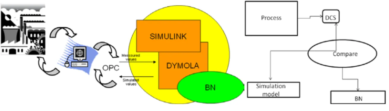
The simulation model is interfaced with Matlab/ Simulink that will get the historical data from the process server. In the same way the results from the simulation will be stored in the process database through Matlab/ Simulink. Figure 3 shows how the on-line application works.
Figure 3. Application overview and Simulation in parallel with the process.
Data from the process is stored in the process database and is visualized in the operators display. OPC (Object link embedment for Process Control), which establishes the communication between plant data and plant equipment. A DYMOLA object is created in Matlab, which can be run using Matlab OPC server against ABB 800xA-environment at Mälarenergi. The results from the simulation are sent to the Data base and the difference between the simulated and the measured data is used as input data into a Bayesian Networks model.
Results and discussion
The model was tuned towards the real process by comparing simulation results to process data. This was performed during May and up to mid June2010 when the plant was closed for the season. When the plant was starting up in September again the system was working and tests were made on-line during first the period 20-23rd September and later 24th September to 4th October continuously without
any stops.
The first variable studied was steam temperature after HPSH2. During the first 24 hours the deviation between predicted and measured temperatures shows a stable temperature difference of 11 °C between the simulated and the meassured data. This deviation can be due to a different fuel composition or a slightly different heat transfer than anticipated. The important fact is that the difference is relatively
constant. The downgoing peaks that are seen in Figure 4 after 36 hours, after 48 hours and the last day can be due to operation upsets or problems during the heat transfer operations.
Figure 4. Difference between simulated and measured data for the variable steam temperature after HPSH2, situated just after the cyclone separator. 10 oC means a relative error of 1.2 %.
The rapid deviation indicates a problem for the operators to act directly. That the problem comes back could indicate that there are problems with fouling, and might need other actions like more frequent soot-blowing. We have not had possibility to really check the true cause, so at this moment we only can discuss possible explanations. By elongated tests, we hope to get a chance to verify a true cause later on. Principally the problem also could be poor sensor measurement. By checking if other sensors related to this one in the steam system behave in the same way, we can conclude that the problem is thermo-mechanical. On the other hand if they do not correlate, the problem may be the temperature meter. Principally there is no difference in these analyses if the deviation is large or small between the predicted value and the measured as long as the relation is constant. A problem still is that fouling is affecting especially the first heat exchangers, where there is a lot of dust. When we have frequent soot blowing we need to keep track on these and the time since last blow. This is for the actual heat transfer. If we look at the long term fouling, that is more or less irreversible fouling, this can be followed long term as an average value, or as the value just after last blow.
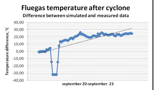
The second pair of variables is shown in Figure 5 and 6. In Figure 5 we see the flue gas temperature after the separator (principally a less efficient cyclone). In Figure 6 we see the temperature before the separator. As the flue gas is a continuum, these two should correlate. To some extent we see a correlation, but not a very strong one. This then indicates that the peaks seen are not related to varying fuel quality, but other type of effects. It is often not easy to identify the relations between different faults and the causes of these. Still, we can make assumptions which we can try to verify by systematic measurements and using the simulator to show what could be expected. The following could be an explanation: 1)The temperature in the flue gas after the separator is first increasing, which could be due to different heat transfer rate in the heat exchangers in the top of the separator the first 48 hours, but stabilizing thereafter. 2) It could also be a drift in a temperature sensor, which is then stabilizing. The strong peak after 18 hours may indicate some mechanical problem in the circulating fluidizing bed with respect to the fluidization. 3) A third cause could be due to combustion high up in the bed due to changes in particle size in the fuel during some period giving after-burning in the top of the separator. It is not selfevident which possible reason is most probable, but as the temperature is stabilising the temperature sensor is probably not the problem.The peak after 18 hours is another problem than the one causing the continuous increase in temperature. Fine fuel particles should have given a much faster increase and thus the most probable of the possible reasons is fouling of heat exchanger surfaces reducing the cooling of the gas. In Figure 6 we have the corresponding temperature before the separator. Here we can see a long term deviation of the temperature indicating a fouling of the temperature meter, and a possible future need for cleaning. We also see that there are several peak deviations indicating spontaneous burning high up in the bed now and then close to the sensor, but probably smoothened out so that this is not seen after the separator.
Figure 5. Difference between simulated and measured data for the variable flue gas temperature after cyclone. 10 oC means a relative error of 0.9 %.
In the simulation we assume a homogenous flow of gas through the exhaust gas channels, but in reality this may be much less stable than assumed. This probably can explain some of the differences. Still, this also can give information about the stability of the flow patterns in the real boiler, which might be of interest to study how e.g. different fuels can effect the flow pattern, as well as where the combustion take place. As fine particles can pass on with the exhaust gas and burn higher up in the boiler or even in the separator it might effect the fouling at different position in the exhaust gas system.
Figure 6. Difference between simulated and measured data for the variable flue gas temperature before cyclone. 10 oC means a relative error of 0.9 %.
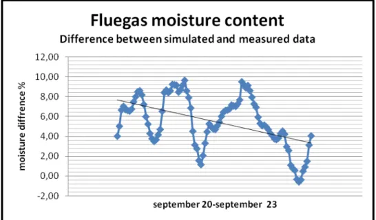
The temperature of the flue gases after the cyclone increases over the studied period of time, while the temperature of the flue gases before the cyclone does not show any corresponding trend. This can indicate combustion in the actual separator. The difference between simulated and measured data for the variable fluegas moisture content, represented in Figure 7, shows an oscillating trend that indicates an alarming behaviour in the several hour to day time-perspective. This variation can be due to changes in the fuel composition, changing load, variations in the air flowrate (poor control),
instabilities in the boiler bed or error in sensor meassurement. The plant was operated under different loads during the four days period (see Figure 8 , from 125 to 165 MW). We don´t see a strong correlation between load and moisture. Concerning moisture measurement we don´t have detailed information as it was not measured frequently. Although the simulation also takes into account varying load, the solids management together with gas strokes with varying conditions is not seen in the simulation and could principally also explain variations.
However, it is possible to see that the difference is being reduced in the long term perspective, over several days. It could be varying moisture content in the fuel or even relation between C and H content in the fuel. More H gives more H2O at combustion. It is not evident which alternative is the correct
one, but the identification of the problem and some alternatives is a good starting point for further investigations. The first dip correlates in time to the temperature dip in temperature after the separator while the lasts dips correlate to disturbances in both steam temperature and temperature dips in temperature before the separator. As it is not correlating to the temperature after the separator it may indicate disturbances in the flow pattern in the exhaust gas channel causing a non-homogenous flow of moisture passing the sensor.
Figure 7. Difference between simulated and measured data for the variable fluegas moisture content.
The analysis made above is an example of how the difference between the values predicted from the model compared to measured values can be used to analyse and diagnose different type of short term or long term problems, both with respect to measurements as such, as well as thermo-mechanical problems in the actual process. In Figure 8 we see the curves together with the boiler load during the time period September 20- September 23. What we can conlude is that there seems to be a correlation between load on the boiler and the temperature before the cyclone, while there is no correlation between the moisture content and the other variables and the load. During the period September 24 to October 4 we made the calculations every one minute without taking the average over the hour. In figure 9 we see the results from this period comparing simulated data to measured data. The bottom curve is the boiler load measured as the fuel feed rate in kg/s. Above that is the temperature before the cyclone, steam temperature after HPSH2, flue gas temperature and at the top flue gas temperature after the cyclcone. As can be seen in the figure the moisture content is not varying . For the gas temperatures we see that these gives lower measured temperatures than predicted at lower loads but higher than predicted at higher loads. The steam temperature after HPSH2 goes the opposite direction. One possible reason can be that we get different heat transfer at HPSH2 at the different loads as the fouling is higher at the higher load. For the higher than expected exhaust gas temperature it may also be due to combustion higher up in the system at the higher load. It might also be that the fuel composition is different at higher loads – dryer or finer particles, or just that the residence time in the bed is lower.
In the next section we will see how this reasoning can be structured in a Bayesian network, which gives the possibility to enhance the knowledge about what is going on inside the boiler in a structured way.
Figure 8 Boiler load vs. Variables during September 20- September 23.The bottom line is flue gas temp before the cyclone at “time 40”, the one above the flue gas temperature after the cyclone, then the moisture content in the flue gas, the steam temperature after HPSH2 and the curve at the top finally is the boiler load (MW).
Figure 9. The second testperiod September 24 to October 4. Comparison between simulation and measured data every minute for all variables except for the fuel feed rate which is in [kg/s]. The curve at the bottom is the flue
gas temperature after the cyclcone. Above that is the temperature before the cyclone, steam temperature after HPSH2, flue gas moisture and at the top we have the boiler load measured as the fuel feed rate in kg/s.
The possible causes to the deviation between predicted and meassured values are configured in a BN and the probability for the different causes is later determined from experience.
Diagnostics results using Bayesian Networks
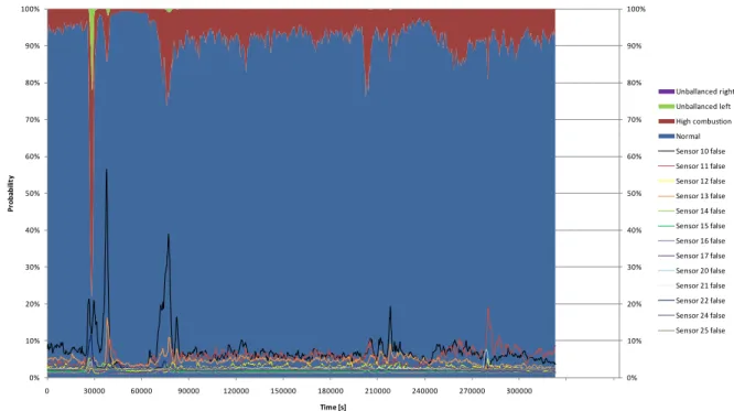
A test run of the Bayesian network with about 4 days of boiler operation September 20-23 gives the results seen in Figure 10. This time period was selected for testing the BN diagnostic system. The boiler was operating at varying load during the test period with loads between 70-90 % of nominal load because there was a time with low heat demand and operation without the steam turbine. The boiler is then cycled during the day, which gives a good indication if the model gives relevant values that correspond to the dynamics.
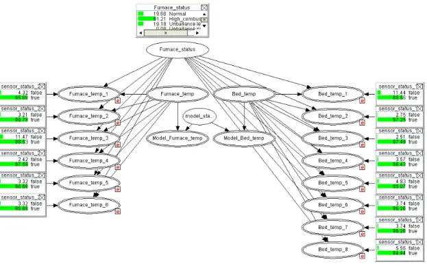
0% 10% 20% 30% 40% 50% 60% 70% 80% 90% 100% 0% 10% 20% 30% 40% 50% 60% 70% 80% 90% 100% 0 30000 60000 90000 120000 150000 180000 210000 240000 270000 300000 Pr ob ab ilit y Time [s] Furnace status Unballanced right Unballanced left High combustion Normal Sensor 10 false Sensor 11 false Sensor 12 false Sensor 13 false Sensor 14 false Sensor 15 false Sensor 16 false Sensor 17 false Sensor 20 false Sensor 21 false Sensor 22 false Sensor 24 false Sensor 25 false
Figure 10. Probability for different type of faults in the CFB boiler for 16 variables as a function of time. Variables with the highest probability for faults are the same ones as seen in figures 8-11.
The coloured area in the graph shows the probability distribution of the node “Furnace status”. “Normal” dominates most of the time, but “High combustion” seems to be quite probable during short time periods. The problem with combustion high up in the boiler is mainly related to fine fuel particles and it can be discussed where the limit is when it becomes a real problem. There is also an indication of unbalance at the left side. Unbalances are usually caused by uneven fuel distribution and it is very interesting in a maintenance perspective. Process data from this time reveals short fuel feeder stops caused by problems in the fuel feeders.
The lines in the graph show the probability of faults in each of the 16 sensor signals. It is clear that some of them have a far more varying fault probability than others. In this situation, it can be interesting to investigate if sensor 10, 11 and 13 is correctly mounted and not disturbed by e.g. air nozzles.
The probability calculations are made by the program HUGIN where the correlation between different variables and the deviation between measured and simulated data are used as input data. The plot in Figure 10 also is one of the presentation views in the HUGIN program.
In figure 11 we see the display from Hugin for the time = 5 when there is very low probability for “high combustion”. There is a 95% probability for normal operations. In Figure 12 we see the presentation from the diagnostic system using the BN where there is a 20 % probability for normal operations but 63 % probability for “high combustion”. In Figure 13 finally we see that the operation looks more normal again. Here we have 78 % probability for normal operation again.
Figure 11. BN at t=5 with 95 % probability that furnace status is in state normal(not high combustion).
Figure 12. BN at t=27900 with 20 % probability that furnace status is in state normal (61 % probability for high combustion).
The boiler load is low when the analysis in Figure 16 is made and the situation here is probably caused by a problem with fuel feeding, causing uneven distribution of fuel.
Figure 13. BN at t=203 400 with 78 % probability that furnace status is in state normal.
The load is in this case normal and the situation with higher temperature in the separator is probably caused by combustion of fine fuel material high up in the furnace.
Conclusions
From the results and discussions we can conclude that it is possible to operate a system on-line where a simulator with a complex physical model is running all the time continuously and calculating predicted values for the different variables in the boiler frequently. We have shown that the model can handle varying loads (Figure 8 and 9, 120-170 MW ) and determine different type of upsets and faults (Figure 4- 7). The deviations have been fed to a Bayesian Network, where the probability for different type of faults is calculated from a BN correlating faults and reasons for the faults in a structured way (Figure 10-13). This BN configuration has to be determined for each specific plant, but the structure is principally the same. The cause of different faults is normally general for a certain type of equipment like a heat exchanger, a cyclone/separator, a fluidized bed etc. The advantage of the application is that the combination of model based diagnostics and decision support can be used to schedule equipment and sensor maintenance. Moreover the application is used on-line which allows evaluation of the system under real circumstances. Results from running the system shows that several different type of faults could be determined simultaneous. Refinement of the probability for the different measurements in relation to different causes are later performed by feeding back knowledge to the BN.
Acknowledgments:
We want to thank Varmeforsk (Thermal Engineering Research Association) for the financial support and valuable inputs from the reference group members. We also want to thank the staff at Malarenergi AB, and especially Peter Karlsson.
References:
[1]
Venkatasubramanian V, Rengaswamy R, Yin K, Kavuri S N; "A review of process fault detection and diagnosis Part I: Quantitative model-based methods",Computers and Chemical Engineering 27, pp 293-311, 2003.
[2]
Venkatasubramanian V, Rengaswamy R, Yin K, Kavuri S N; "A review of process fault detection and diagnosis Part II: Qualitative models and search strategies", Computers and Chemical Engineering 27, pp 313-326, 2003.[3]
Venkatasubramanian V, Rengaswamy R, Kavuri S N, Yin K; "A review ofprocess fault detection and diagnosis Part III: Process history based methods", Computers and Chemical Engineering 27, pp 327-346, 2003.
[4]
Widarsson B¸ Karlsson C, Nielsen, T, ”Bayesian Networks applied to process diagnostics”, Värmeforsk 882, Stockholm October 2004, ISSN 0282-3772.[5]
Avelin A, Jansson J, Dotzauer E. “Use of combined Physical and Statistical Models for On-line Applications in the Pulp and Paper Industry”, Mathematical and Computer Modeling of Dynamical Systems: Methods, Tools and Applications in Engineering and Related Sciences, 1744-5051, v15-5, p. 425 – 434, 2009.[6]
Dahlquist E, Widarsson B, Lilja R, “Dynamisk dataåterförening - kvalitetssäkring av signaler”, Värmeforsk 1050, Stockholm March 2008, ISSN 1653-1248.[7]
Karlsson C, Avelin A, Dahlquist E, ”How to make better use of all the process data collected in process industry and power plants”, 6th Eurosim Congress on Modeling and simulation, , Ljubljana, Slovenia, September 2007.[8]
Karlsson C, Dahlquist E;”Process and Sensor diagnostics”, Värmeforsk 834, Stockholm October 2003, ISSN 0282-3772.[9]
Weidl, G., Madsen, A.L. and Dahlquist, E. (2002), “Bayesian Networks for Root cause analysis in process operation”, European Journal of Operational Research, Special issue on “Advances in Complex System Modeling”.[10]
Widarsson B, Dotzauer E; “Bayesian Networks-based early-warning for leakage in recovery boilers”, Applied Thermal Engineering, v.28-7, p. 750-764, May, 2008.[11]
Widarsson B, Dotzauer E, Dahlquist E; “System för tidig läckagevarning i sodapanna”, Värmeforsk 986, Stockholm, December 2006, ISSN 1653-1248.[12]
Man Cheol Kim, Poong Hyun Seong; “An analytic model for situation assessment of nuclear power plant operators based on Bayesian inference”, Reliability Engineering & System Safety, Volume 91, Issue 3, March 2006, Pages 270-282[13]
Giovanni Cerri_, Sandra Borghetti, Coriolano Salvini, “Neural management for heat and power cogeneration plants“, Engineering Applications of Artificial Intelligence 19 (2006) 721–730[14]
Ciarapica F.E. , G. Giacchetta: Managing the condition-based maintenance of a combined-cycle power plant: An approach using soft computing techniques. Journal of Loss Prevention in the Process Industries 19 (2006) 316–325[15]
Struss P, Provan G, de Kleer J, ; ”Special issue on Model-Based Diagnostics”, IEE Transactions on Systems, Man and Cybernetic part A:Systems and Humans, Volume 40, Issue5, , 870-873, September 2010.[16]
Jensen, F V, "Bayesian Networks and decision graphs"; Springer-Verlag 2001 ISB 0-387-95259-4.[17]
Norsys Software Corp., Netica Tutorial, Norsys Sotware Corp.,http://www.norsys.com/tutorials/netica/nt_toc_A.htm, 2010-12-02
[18]
Fritzon, P., 2007, “Modelica – A unified Object-Oriented Language for Physical Systems Modeling, Language Specification Version 3.0”, The Modelica Association.[19]
Dynasim AB, 2004-2009, 20090308, www.dynasim.com/dynasim htm[20]
Modelon AB , Ideon Science Park , SE-22370 LUND, Swedenhttp://www.modelon.se/.[21]
Otter, M. and Elmquist, H., 2001; Modelica – Language, Library, Tools, Workshop and EU-Project RealSim.Paper 4
Title: Retention time and nutrient tracking inside a digester for biogas production
Johan Lindmark, Rebei Bel Fdhila, Eva Thorin
Mälardalen University, Sweden
Keywords: Biogas, Mixing, Digester, CFD, Retention time, Nutrition
A large proportion of today’s biogas plants are continuous stirred tank reactors (CSTR) and
they are usually assumed to be perfectly mixed. Based on this assumption the retention time
of the biogas plants and the organic loading rate are estimated. However, there can be large
inconsistencies in the mixing parameters leading to local variations in the mixing pattern and
in mixing intensity. These variations can lead to an uneven distribution of nutrients and
microbiological activity inside the digester.
The digester is the heart of the biogas process where the organic material is broken down in
steps to simpler compounds and finally to the energy rich gas methane. By controlling the
environment for the microorganisms inside the digester the fermentation process can be
improved with an increased capacity as a result. The mixing inside the digester is one of the
most important measures of control available.
Several investigations have shown that the mixing inside the digester has a direct effect on the
biogas yield and that the result is affected by the dry solid content of the mixture. At low dry
solid content the mixing could possibly be handled by the naturally occurring mixing and only
small improvements can be made by increasing the mixing.
Mixing becomes more important at higher total solid content and can affect the gas yield
considerably. Previous studies, using a manure slurry with a total solid content of 10% as
substrate, have shown that increased mixing can improve the gas yield by 29%, 22% and 15%
compared to an unmixed digester by mixing with slurry recirculation, impeller mixing and gas
injection respectively. Higher total solid contents can of course also lead to other problems in
an unmixed digester like sedimentation or problems with a flouting layer.
In this study the retention time and dispersion of the feed inside the digester at the Växtkraft
biogas plant in Västerås, Sweden, is studied using Computational Fluid Dynamics (CFD) to
understand the effect that the mixing has on the process. This work provides the distribution
of nutrition and how the nutrient disperses inside the digester. The impact of mixing is
evaluated by comparing experiments and simulations of the flow and mixing intensity with
simulations of the nutrient content inside the digester.
Retention time and nutrient tracking inside a digester for biogas production
J. Lindmark1, R. Bel Fdhila1,2, E. Thorin1
1Mälardalens University, Energy division, School of Sustainable Development of Society and Technology,
Västerås, Sweden; 2ABB AB, Corporate Research, SE - 721 78, Västerås, Sweden
Corresponding Author: J. Lindmark, Mälardalens University, School of Sustainable Development of Society and Technology, Box 883, 721 23 Västerås, Sweden: johan.lindmark@mdh.se
Abstract. A digester is practically a black box with too few possibilities to study what is going on inside. The continuous stirred tank reactor (CSTR) is a common digester design for biogas production which puts a high demand on the mixing configuration. This type of digester design is often assumed to be perfectly mixed which influences operational decisions e.g. residence time which can lead to problems in the process and low capaci-ties. Chemical tracer methods have been used to study the mixing at biogas plants to give valuable information on retention time, active volumes and short-circuiting in plants already in operation but it is time-consuming and costly to make these types of evaluations. In this work the retention time and dispersion of the feed inside a di-gester is studied using a Computational Fluid Dynamic (CFD) model. A scalar is injected in the simulation to mimic the tracer method and to see the effect that the mixing has on dispersion of nutrient in a pneumatically mixed digester. The conclusions from this study are that large dead and stagnant zones can be found in the di-gester, as much as 30 %. The mixing configuration studied is limiting the dispersion of nutrient to 30 – 40 % of the digester because of the barrier that the column of bubble produces. One way to improve the dispersion could be to have two or more injection points. It takes the nutrient/feed around 125 seconds to follow the entire circula-tion path of the mixing and return to the starting point around the gas injectors.
Keywords: CSTR, CFD, HRT, biogas, mixing, digester, feed, nutrition, tracer
1 Introduction
A large proportion of today’s biogas plants are continuous stirred tank reactors (CSTR) (De Baere 2010, Weil-and 2010) Weil-and they are usually assumed to be perfectly mixed. Based on this assumption the retention time of the feedstock in the biogas reactor as well as the organic loading rate is estimated. However, there can be large in-consistencies in the mixing leading to variations in the mixing pattern and in mixing intensity (Karim et al. 2007, Lindmark et al. 2008). These variations can lead to stagnant zones, sedimentation, flotation and short-circuiting in the digester as well as an uneven distribution of nutrients and microbiological activity.
The digester is the heart of the biogas process where the organic material is broken down in steps to simpler compounds and finally to the energy rich gas methane. By controlling the environment for the microorganisms inside the digester the fermentation process can be improved with an increased biogas yield as a result. However, the biological process is complex and controlling it is a challenge.
The mixing inside the digester has been shown to be an important control measure of the process. Several inves-tigations have shown that the mixing has a direct effect on the biogas yield but there are many contradicting opinions on how the mixing should be designed for best results. There are studies that show positive effects both from increasing (Karim et al. 2005a) and decreasing (Stroot et al. 2001) the mixing. High mixing intensities and shear have been shown to have negative effect on the microorganisms and the formation of flocks inside the digester (McMahon et al. 2001, Whitmore et al. 1987, Dolfing 1992).
The effects of mixing on the mass transfer and the digestion process are strongly connected to the content of total solids, viscosity and rheological properties of the digestate (Karim et al. 2005a, Karim et al. 2005b, Karim et al. 2005c) and this puts a high demand on the mixing equipment used (Yu et al. 2011). At low dry solid content the mixing could possibly be handled by the naturally occurring mixing and only small improvements can be made by increasing it
(
Karim et al. 2005a)
. Mixing becomes more important at higher total solid content and can affect the gas yield considerably. Previous studies, using a manure slurry with a total solid content of 10% as substrate, have shown that increased mixing can improve the gas yield by 29%, 22% and 15% compared to an unmixed digester by mixing with slurry recirculation, impeller mixing and gas injection respectively(
Karim et al. 2005b)
. High total solid contents can of course also lead to other problems in an unmixed digester like sedimentation or problems with flotation.The digester is basically a black box with few or no possibilities to evaluate the result of the mixing. The hydrau-lic retention time, the dispersion of the feed, stagnant zones and short-circuiting can be analyzed by using a trac-er method. In this method you add a chemical tractrac-er (e.g. lithium chloride) that is mixed with the injected liquid and by analyzing the concentration of this tracer at the outlet conclusions of the mixing quality can be drawn. This method is time-consuming and costly and that is why the use of a Computational Fluid Dynamic (CFD)
model has been proposed by many researchers as an alternative to this method (Meroney and Colorado 2009, Terashima et al. 2009).
In this study the retention time and dispersion of the feed inside a digester is studied using a CFD model. A trac-er is injected in the simulation to see the effect that the mixing has on disptrac-ersion of nutrient. This work provides information on how the distribution of nutrition looks like and short-circuiting effects in a pneumatically mixed digester.
2 Computational model
To simulate the movement of the fresh feed inside a digester the volume of fluid (VOF) approach was chosen. A two phase gas/liquid, transient and turbulent model was built to visualize and analyze the local process changes at different time instants. The geometry of the digester was built, specifying appropriate boundary conditions at inlets and outlets. A passive scalar was injected through the liquid inlet as a tracer to be able to follow the disper-sion of nutrient/feed inside the digester.
2.1 Digester Geometry
The simulated digester is a cylindrical CSTR with a radius of 8.5 m and a height of 19.5 m and a total liquid volume of 4 000 m3. Mixing of the liquid is done pneumatically by compressing biogas and distributing it through 12 injection pipes that release the gas at the bottom, in the center of the digester, the gas is then recov-ered at the top. The liquid inlet is situated near the bottom close to the side wall and the outlet at the bottom at the center of the digester. The inlet and outlet pipes were added as small sections of cuboids to facilitate that a good mesh quality could be produced.
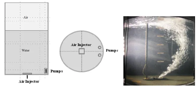
Figure 1. Illustration of the geometry that was used in the simulations. The left showing the shape of the digester with the
positioning of the liquid outlet (centre) and liquid inlet (on the right hand side). The right picture is showing the top view of the digester bottom and the 12 gas injection points as well as the angles of the liquid inlet and outlet. The gas is injected facing out from the centre through the injection pipes and the liquid is pumped in and sucked out directed towards the centre.
The mesh was built up as a mixture of hexahedral and of tetrahedral cells, dividing the entire domain in 436 000 individual volumes in a structured way. A finer mesh was built at the bottom around the liquid inlet and outlet as well as around the gas injection pipes for better resolution in these areas where the gradients are high and the flow changes can be fast.
2.2 Boundary conditions
The gas inlets are all set to mass flow inlets with a specified mass flow rate. The liquid inlet and outlet are mod-eled as velocity inlets with the same fixed value to ensure that the introduced liquid is extracted. The gas outlet was set as a pressure outlet to allow the gas to be removed from the digester. The surface of the digestate was simulated as a free surface with a meniscus between the liquid and gas filled headspace. The boundary condi-tions are presented in Table 1.
Table 1. Boundary conditions.
Boundary Type value
Gas injection pipes Mass flow inlet 0.01747 kg/s Liquid inlet Mass flow inlet 1.349 m/s Liquid outlet Mass flow inlet -1.349 m/s
Gas outlet Pressure outlet -
Digester walls No slip -
2.3 Mathematical model
The VOF model was used to be able to track the two immiscible fluids using a single set of momentum equa-tions. This model is used when the position of the interface between two fluids is of interest like in this case. The numerical solution can show the dispersal pattern of the feed and how much time it takes for the feed to reach the liquid outlet and be removed from the system.The turbulence is modelled using Reynolds stress model.
The model was set up using the physical properties of water because of the high water content (above 95 %) of the digester and the uncertainties in the property of the digestate. Thicker digestate puts a much higher demand on the mixing configuration and by using the properties of water we can see the imperfections in the mixing before they are magnified by higher TS. The physical properties of air were used for the properties of the in-jected gas.
To be able to track the flow of incoming feed a passive scalar in the liquid phase was injected through the liquid inlet after 327 seconds of the simulation and the concentration of the scalar in the digester are be tracked as it is mixed with the digestate. By analyzing the scalar in the different time steps the accumulation and deficiency of nutrients inside the digester can be visualized and recorded. Short-circuiting of the flow, leading to loss of fresh feed and nutrients, can be recorded at the vicinity of the liquid outlet.
2.4 Convergence
The flow is naturally transient however a stable solution is reached at approximately 5 minutes physical time. The flow was then frozen and the scalar was injected in a continuous manner with the liquid feed. At the inlet a scalar constant value of 1.0 was used.
3 Results and discussion
3.1 Mixing dynamicsThe nutrient will follow the liquid circulation pattern which is produced by the mixing equipment and will be dispersed throughout the domain. To understand the mechanisms of the nutrient dispersion there is a need to study how the mixing is functioning and the flow field it produces. In the pneumatic configuration studied the gas is injected at the bottom and the buoyancy of the gas will cause the bubbles to rise towards the surface while transferring momentum to the liquid. The injected gas can be seen in figure 2 like a plume of rising bubbles. The coarse mesh that we use influences certainly the size of these created bubbles or even gas pockets. The smaller the mesh cells the better accuracy of the gas bubbles description. However, we need to keep the mesh size under control to have a reasonable simulation time.
Figure 2. Tracking the flow of bubbles as volume fraction of gas in the liquid. The left figure is showing the bubbles or gas
pockets path at the vertical mid-plane and the right figure is showing the volume fraction of gas in the tank at 5, 10 and 15 m from the bottom with the red colour representing the highest fraction of gas (5%) and blue the lowest (only liquid).
The results of the mixing and the flow fields can be seen in Figure 3, showing the velocity vectors and velocity contours inside the entire domain of the digester. The results clearly show that there is a good vertical circula-tion. There is a high liquid speed produced in the centre of the digester, up to 1 m/s, and there is a recirculation of liquid along the sides of the digester. However, there are areas that virtually have no mixing and large areas with very low liquid speed. There are some turbulent areas where numerous vortices are formed close to the free surface of the liquid and also at the bottom. The flow field ranges from a speed of 0 m/s to 1 m/s. The really high flows can be seen in the stream of bubbles while the periphery only has a speed of a couple of cm per second and totally stagnant zones in some places. The grey circle at the top of the digester outlines the meniscus of the di-gester and the vectors above that line illustrates the gas phase with the gas outlet in the centre of the top wall.
Figure 3. velocity vectors and velocity contours of the liquid phase. The figure is showing the velocity vectors in the digester
to see in which direction the liquid is flowing with fixed vector size (top left) and also showing the real size of the vector (top right). The figure is also showing the velocity contours with (bottom left) and without filling (bottom right). The colour
indi-cates a liquid speed range is between 0- 1 m/s (blue – red).
3.2 Tracking the dissolved nutrient
Tracking the dissolved nutrient inside the digester by means of the CFD tracer method shows a good vertical mixing of nutrient (Fig 4) as suggested by the mixing dynamics and earlier studies (Lindmark et al. 2008). How-ever, the configuration of the feed/nutrient injection (from the left side in this figure) leads to an uneven distribu-tion of nutrient. The scalar was first injected after 327 seconds of mixing so that the flow fields had time to stabi-lise and in this figure the nutrient dispersal can be seen at different time instants (from left to right). The second time illustrated (at 487 seconds) is approximately the time were the nutrient has made its way back to the injec-tion point
Figure 4. The scalar tracer at different time instants, shown as concentration of the scalar in the digestate. The figure shows
the distribution of the nutrient at 407 (T1), 487 (T2) and 543 (T3) seconds from left to right. Showing the dissolved nutrients path through the digester with the red colour representing the highest concentrations and blue the lowest (0-0.05).
To get more details on the nutrient dispersal the range of concentration was changed to 0 - 0.01 at time T3 and
also viewed in the z-direction at 2, 5, 10 and 15 m from the bottom (Fig 5). From this it can be concluded that the nutrient is only dispersed efficiently in around 30 - 40% of the digester and the rest of the volume is under-nourished. Overloading could possibly be a problem in the areas where we have the dispersion of nutrient since there will be an accumulating effect.
Figure 5. Dispersion and accumulation in the digester. Contours of the scalar concentration in the range 0 – 0.01.
Using a scalar as a tracer in the simulations has both benefits and drawbacks. Using a scalar is very similar to the use of the tracer method which means that it is accepted by the industry but it also gives a wide range of data concerning the dispersion of nutrient that the tracer method never could do. In the CFD simulation we can study the concentration of nutrient at every moment of the process and every part of the digester and visualize the results. When working with a passive scalar and using an imposed velocity boundary condition at the outlet, we need to set in advance a value for the scalar at that boundary. This means that the exact time when the scalar starts to be evacuated at the outlet is difficult to find out and evaluate operating parameters like e.g. the retention time. Because of this it is more appropriate to study dynamics in the system than for operational data like hy-draulic retention time (HRT) and solid retention time (SRT) even though some conclusions about them can be drawn. By studying the concentration changes of the scalar at the gas injectors (positioned around the liquid
outlet) the turn over time can be seen as well as some effects of short-circuiting flows inside the digester (Figure 6). There is a stable concentration of the scalar around the gas injectors directly from the time of injection which is caused by short-circuiting and it is 1.15 % of the scalar mixed with the liquid that probably will be removed from the digester through the liquid outlet. At T = 452 there is a rapid increase in the concentration of the scalar after it has gone through the entire digester and returned to the source of the mixing, the turn over time. The turnover time of the scalar is consequently near to 125 seconds and the path the scalar will take can be seen in the velocity vectors in Figure 3.
Figure 6. Turn over time of the digester. This figure shows the volume fraction of the scalar around the gas injectors changes
with time.
From an engineering point of view it is very hard to control a biological process because there are so many fac-tors influencing the process. There has been some work done to evaluate the effects of mixing both by microbi-ologists and engineers but there is as of yet no coherent picture on what actions to take to get the improved di-gestion process that everyone is aiming for.
The impact of mixing on parameters like temperature, pH and retention time in the digester seems to be a good starting point from which to analyze the effects of the mixing imperfections. One of the main possibilities for control is the addition of fresh feed but because of mixing imperfections we can have overloaded and undernou-rished zones in the digester at the same time even if the organic loading rate to the digester itself is adequate. There is also the possibility that inhibiting substances can accumulate in the digester and that inconsistencies in temperature and pH can form within the digester with local effects on the microorganisms. All these parameters have been extensively studied and there is a good theoretical basis from which to draw conclusion. By consider-ing mass transfer, physical properties and the mixconsider-ing in the digester the effects of the different parameters can be studied in every part of the digester, as a matrix.
Vesvikar and Al-Dahhan (2005) suggests that all areas with a mixing below 5 % of the maximum is stagnant or dead zones which has negative effects on the biogas plants capacity to produce biogas. In this simulation around 30 % of the total volume would fall under that category (two darkest shades of blue in figure 3). Except for the effect of mixing on mass transfer they also mean that these zones lead to the degradation of digester performance by increase in pH and temperature.
It is also possible to study the temperature range inside the digester through simulations but the pH is directly connected to the microbiological activity and the concentration of nutrient which makes it harder to predict. However, valuable information on the dynamics of the digestion could be gained by studying it.
4 Conclusion
There are large dead and stagnant zones in the digester and according to the preliminary simulations made on mixing dynamics result say it can be around 30 %.
The mixing configuration is limiting the dispersion of nutrient to 30 – 40 % of the digester because of the barrier that the column of bubble produces. One way to improve the dispersion could be to have two or more injection points.
It takes the nutrient/feed that is pumped in to the digester around 125 seconds to follow the entire circulation path of the mixing (Fig 3) and return to the zones around the gas injectors.
5 Acknowledgement
This study was funded by the European Regional Development Fund through the project Regional Mobilizing of Sustainable Waste-to-Energy Production (REMOWE) which is a part of the Baltic Sea Region programme.
6 References
Dolfing, The energetic consequences of hydrogen gradients in methanogenic ecosystems, FEMS Microbiol. Ecol. 101 (1992), 183–187
Karim, K., Varma, R., Vesvikar, M., and Al-Dahhan, M.: Flow pattern visualization of a simulated digester. Water Research, 38(17) (2004),3659-3670.
Karim, K., Klasson, K.T., Hoffmann, R., Drescher, S.R., DePaoli, D.W., Al-Dahhan, M.H., Anaerobic digestion of animal waste: Effect of mixing. Bioresource Technology, 96(14) (2005a), 1607-1612
Karim, K., Hoffmann, R., Klasson, T., Al-Dahhan, M.H. Anaerobic digestion of animal waste: Waste strength versus impact of mixing. Bioresource Technology 96 (16) (2005b), 1771-1781
Karim K., Hoffmann R., Klasson K.T., Al-Dahhan M.H., Anaerobic digestion of animal waste: Effect of mode of mixing, Water Research, 39 (15) (2005c), 3597-3606.
Karim, K., Thoma, G. J., and Al-Dahhan, M. H.: Gas-lift digester configuration effects on mixing effectiveness. Water Research, 41(14) (2007), 3051-3060.
Liang Yu, Jingwei Ma and Shulin Chen, Numerical simulation of mechanical mixing in high solid anaerobic digester, Bioresource Technology, 102 (2) (2011), 1012-1018
Lindmark J., Bel Fdhila R., Thorin E., On modelling the mixing in a digester for biogas production. In Proceed-ings of MATHMOD 09, 6th International Conference on Mathematical Modelling, Vienna, Austria, 2009. McMahon, K.D. , Stroot, P.G., Mackie, R.I., and Raskin, L., Anaerobic codigestion of municipal solid waste and biosolids under various mixing conditions-II: microbial population dynamics, Water Res. 35 (7) (2001), 1817– 1827.
Meroney, R.N., Colorado, P.E.CFD simulation of mechanical draft tube mixing in anaerobic digester tanks Water Research, 43 (4) (2009), 1040-1050
Terashima M., Goel R., Komatsu K., Yasui H., Takahashi H., Li Y.Y., Noike T., CFD simulation of mixing in anaerobic digesters, Bioresource Technology, 100 (7) (2009), 2228-2233.
Stroot, P.G., McMahon, K.D., Mackie, R.I., Raskin, L., in press. Anaerobic codigestion of municipal solid waste and biosolids under various mixing conditions-I. Digester performance, Water Res. 35(7) (2001), 1804–1816. De Baere, L., Mattheeuws, B., and Velghe, F. (2010). State of the art of anaerobic digestion in Europe, 12th World Congress on Anaerobic Digestion, October 31st –November 4th, Guadalajara, Mexico.
Vesvikar, M.S., Al-Dahhan, M., Flow pattern visualization in a mimic anaerobic digester using CFD. Biotech-nology and Bioengineering 89 (6) (2005), 719–732.
Weiland, P., Biogas production: current state and perspectives, Applied Microbiology and Biotechnology, 85 (2010), 849–860.
Whitmore, T.N., Lloyd, D., Jones, G. and Williams T.N., Hydrogen-dependent control of the continuous anae-robic digestion process, Appl. Microbiol. Biotechnol. 26 (1987), pp. 383–388.