Application of game theory in Swedish raw material market: Investigating the pulpwood market

Application of game theory in Swedish raw

material market

Investigating the pulpwood market

Rami Al-Halabi

Dokumenttyp – Självständigt arbete på grundnivå

Huvudområde: Industriell organisation och ekonomi GR (C) Högskolepoäng: 15 HP

Termin/år: VT2020

Handledare: Soleiman M. Limaei Examinator: Leif Olsson

Sammanfattning

Studien går ut på att analysera marknadsstrukturen för två industriföretag (Holmen och SCA) under antagandet att båda konkurrerar mot varandra genom att köpa rå material samt genom att sälja förädlade produkter. Produktmarknaden som undersöks är pappersmarknaden och antas vara koncentrerad. Rå materialmarknaden som undersöks är massavedmarknaden och antas karaktäriseras som en duopsony. Det visade sig att Holmen och SCA köper massaved från en stor mängd skogsägare. Varje företag skapar varje månad en prislista där de bestämmer bud priset för massaved. Priset varierar beroende på region. Både SCA och Holmen väljer mellan två strategiska beslut, antigen att buda högt pris eller lågt pris. Genom spelteori så visade det sig att båda industriföretagen använder mixade strategier då de i vissa tillfällen budar högt och i andra tillfällen budar lågt. Nash jämviktslägen för mixade strategier räknades ut matematiskt och analyserades genom dynamisk spelteori. Marknadskoncentrationen för pappersmarknaden undersöktes via Herfindahl-Hirschman index (HHI). Porters femkraftsmodell användes för att analysera industri konkurrensen. Resultatet visade att produktmarknaden är koncentrerad då HHI testerna gav höga indexvärden mellan 3100 och 1700. Det existerade dessutom ett Nash jämviktsläge för mixade strategier som gav SCA förväntad lönsamhet 1651 miljoner kronor och Holmen 1295 miljoner kronor. Dynamisk spelteori visade att SCA och Holmens budgivning följer ett mönster och att högt/lågt bud beror på avvikelser från Nash jämviktslägets sannolikhetsdistribution. Nash jämviktslägets råder ifall sannolikhetsdistributionerna vid låg budgivning är 68,6 procent för SCA och 66,7 procent för Holmen. Detta gav indikatorer för icke samarbetsvilliga spel. Slutsatsen är att om två spelare (kvarnar) når Nash-jämvikten, kommer ingen spelare att vinna mer genom att bara ändra sin egen strategi.

Nyckelord: Spelteori, Herfindahl-Hirschman index (HHI), duopsony,

Abstract

The research aims to analyze the market structure of two companies in the forest industry (Holmen and SCA) with the assumption that these companies compete at buying raw materials and selling products. The product market in this study is the paper market under the assumption that both companies operate in a concentrated product market. The raw material market that one investigates in this study is the pulpwood market under the assumption that it is a duopsony. What this study has concluded is that Holmen and SCA buy pulpwood from lots of different self-managing forest owners. Each company creates a monthly pricelist where they decide the bid price of pulpwood. The amount varies depending on the region. Both SCA and Holmen chooses between two strategic decisions, either to bid high or to bid low. Through game theory, it has been clear that each company uses mixed strategies as they sometimes give high bids and sometimes give low bids. The Nash equilibrium for mixed strategies have been calculated mathematically and analyzed through the dynamics of game theory. As for the market concentration, the product market has been investigated through the Herfindahl-Hirschman index (HHI). Porter's five-force model was used to analyze the industry competition. The results showed that the product market is concentrated as the HHI tests gave High index scores between 3100 and 1700. In addition, there existed a Nash equilibrium in a mixed strategy that gave SCA expected payoff 1651 million SEK and Holmen 1295 million SEK. The dynamic game theory showed that SCA and Holmen's bidding follows a repeating trajectory and that the high/low bidding is due to deviations from Nash equilibrium probability distribution. The Nash equilibrium situation prevails if the probability distribution at low bidding is 68.6 percent for SCA and 66,7 percent for Holmen. This provided indicators for a non-cooperative game. The conclusion is that if two players (mills) reach the Nash equilibrium, no player will gain more by changing only their own strategy.

Keywords: Game theory, Herfindahl-Hirschman index (HHI), duopsony,

Preface

This study has been inspired by the previous work of my supervisor Dr. Soleiman Mohammadi Limaei. Therefore, I would like to express my sincere thanks to his excellent guidance in this research.

Content

2.2.1 The theory of the firm ... 5

2.2.2 Pulp and paper industry ... 6

2.2.3 Competitive and Non-competitive markets ... 6

2.2.4 Porter's five forces ... 6

2.2.5 Market structure ... 8 2.2.6 Cartel... 8 2.2.7 Payoff calculation ... 9 2.2.8 Herfindahl-Hirschman Index ... 9 2.3 Regression analysis ... 9 2.3.1 Multiple regression ... 10 2.3.2 Hypothesis testing ... 10 2.3.3 Goodness of fit ... 10 2.4 Game theory ... 11 2.4.1 Game definition ... 11

2.4.2 Strategic game and Extensive game ... 12

2.4.6 Mixed strategy Nash equilibrium ... 13

2.4.7 Best response functions in two-player two-action games ... 13

2.4.8 Duopsony game ... 14

2.4.9 Cases in duopsony games ... 15

2.4.10 The expected payoff in a mixed strategy ... 15

2.4.11 Expected payoff hypothesis ... 15

2.5 Previous research ... 16 3 Method ... 17 3.1 Overall method ... 17 3.2 Excel ... 17 3.3 Draw.io ... 17 3.4 Data collection ... 17 3.5 Selections of variables ... 18 3.5.1 Dependent variable ... 18 3.5.2 Independent variables ... 18 3.6 Herfindahl-Hirschman Index ... 18 3.7 Regression model ... 19

3.7.1 Formulating the profit equations ... 19

3.8 Expected payoff equation and Nash equilibrium ... 20

3.8.1 Expected payoff hypothesis test ... 20

3.9 Dynamics of the mixed strategy game ... 20

3.10 From data to a Game theory application ... 21

3.11 Method discussion ... 22

3.11.1 Reliability ... 22

3.11.2 Validity ... 22

3.12 Ethical and societal aspects ... 23

4 Results ... 24

4.1 SCA regression data ... 24

4.2 Holmen regression data ... 25

4.3 SKOGEN regression data ... 26

4.8 SCA regression results ... 30

4.9 Equations ... 31

4.10 Game theory applications... 32

5 Discussion ... 36

6 Conclusion ... 39

7 Further research ... 39

Terminology

Microeconomics

Microeconomics deals with the behavior of various distinct economic units. These units can consist of consumers, workers, investors, landowners, and companies. Microeconomics enlightens how and why these units make financial choices. Another significant component is by what means industrial units cooperate to form more significant groups, markets, and

industries [1]. Industry

An industry is an assembly of corporations that together sell the same or similar products. The sector has its effect on the supply side of the market [1].

Market

A market is an assembly of buyers and sellers who collectively determine the price of goods [1].

Buyers and Sellers

Buyers consist of consumers who purchase items or services and corporations that buy work, capital, and raw materials. Sellers are corporations that sell items and services but also land or resource owners who sell resources or land to other corporations [1].

Arbitrage

Once someone buys low-priced from one area to later sell much more expensive somewhere else is called arbitrage [1].

Payoff

A payoff can be seen as a favorable value related to action-based outcomes. E.g., profit or rewards that the company generates by lowering prices and increasing quantity or buying cheap and selling high [1].

Prices

In a market economy, the price is determined through interactions between consumers, workers, and companies. These interactions occur in a market. The equilibrium price is the price in which the quantity supplied equals quantity demanded [1].

Acronyms

PPI

Industrial Organization Pulp and Paper Industry HHI VNM EBITDA MSEK Kton MR ha Herfindahl-Hirschman Index Von Neumann-Morgenstern

Earnings before interest, taxes and depreciation and amortization

Millions of SEK Kiloton

Multiple regression hectare

1 Introduction

On the market's supply side, an oligopoly arises as a market structure when the market has only a few sellers and many buyers. The intense market concentration of these few sellers is similar to a monopoly situation where there are only one seller and many buyers. Something that one rarely discusses is the market structure on the demand side of the so-called "mirror market." The mirror market for a market considered as a monopoly is called a monopsony. There exist only one buyer and many sellers in the monopsony market. The mirror market for a market viewed as an oligopoly is called oligopsony. This market consists only of a few buyers and many sellers.

Oligopoly competition has a significant role in industrial organization (IO), yet the mirror concept oligopsony seems to be rarely mentioned. Two reasons seem to explain this, partly because there is a lack of interest in the buyers' market power and because it is not considered to give any unique modeling problems relative to the sellers' market power [3].

1.1 Background

A lot of Sweden's lands consist of forests. Sweden's total area is 40.8 million hectares (ha), and 57 percent is productive forest land. A significant share is owned by private forest owners and is usually inherited from generation to generation. The forest industry is of immense importance to the Swedish economy [4].

Sweden is one of the world's largest exporter of pulp, paper, and sawn timber. With a relatively small population, Sweden can still be seen as a forest nation due to its efficient production. The forest industry utilizes millions (cubic meters) of domestic raw materials. Approximately half of the raw materials is sawn timber, and the other half is pulpwood [5]. Wood markets are divided into three types of markets roundwood, pulpwood, and saw timber. Pulpwood and saw timber are two separate submarkets of the roundwood market [6]. Wood is acquired according to two different types of agreements. The market of delivered wood, which means that the forest owners (sellers) harvest and drive the wood to a pickup point. The buyer collects it by road and transports it to the industry. Payment is made agreeing to a pricelist offered by the buyers. The second market is the market of the felling mission. It is similar to the market for delivered wood, but the difference is that the buyers themself are responsible for harvesting. The cost of the crop is subtracted from the payment [7].

1.2 Corporate information 1.2.1 SCA

SCA has three paper mills. Munksund paper mill, Ortviken paper mill, and Obbola paper mill. Munksund has a total capacity of 400,000 tons per year [8]. Ortviken has a full capacity of 756,000 tons per year [9]. Obbola has a full capacity of 450,000 tons per year [10]. The mills are located in three different parts in the north of Sweden (Figure 1).

Figure 1. The location of SCA:s paper mills. The dark green area represents forests that supply SCA's paper mills with raw materials [11].

1.2.2 Holmen

Holmen has two paper mills. Braviken paper mill and Hallsta paper mill. Hallsta has a total capacity of approximately 800,000 tons per year [12]. Braviken has a full size of roughly 600,000 tons per year [13]. The mills are located in two different parts in the middle and south of Sweden (Figure 2).

Figure 2. The location of Holmens paper mills. The yellow area represents the southern region, and the orange area represents the middle region. Both regions provide the raw material for Holmen's paper mills [14].

1.3 Overall purpose

The purpose of this study is to investigate and analyze the market structure of the forest industry's raw material market in Sweden and to measure market concentration in Swedish pulp and paper industries (PPI).

1.4 Delimitations

This study is restricted to examining two industry's SCA and Holmen under the assumption of duopsony. The raw material market is limited to the pulpwood market. The purchase of raw materials is restricted to two geographical regions in Sweden (Va sternorrland and Ha lsingland). Data is

1.5 Goal

The goal of this study is to investigate the raw material market by constructing a two-person, non-zero-sum game between two competing companies in Sweden. The expected results are that the product market is concentrated and that the pulpwood bids of each company may influence profits and that there exists a Nash equilibrium either in pure strategy or in a mixed approach. The report will answer the following questions:

• What is the degree of competition in the paper market? • What are the properties of the pulpwood market under the

duopsony assumption?

1.6 Contribution

The main research object is the duopsony game theory model, usually used for duopoly market analysis. The research method is an efficient science literature investigation, and the structure of the paper is based on the works of Mohammadi Limaei and Lohmander that made similar forest industry investigations but with different empirical data. The paper is also influenced by the work of VNM, Nash, Cournot, and many more authors who have contributed substantially to the development of game theory and its application.

2 Theory

This chapter mentions various theoretical methods, tools, and definitions used in the field of microeconomics and game theory.

2.1 Problem description

The pulpwood market in Sweden is functioning in some cases under imperfect competition. It is because of the high concentration of buyers on the demand side. At the same time, the supply side is more split between a lot of sellers [6]. This notion has led to the assumption that the market structure is an oligopsony or a regional monopsony [15].

Market demand for forest raw materials has been observed to be concentrated in the hands of a few industries the low rate of competition gives the assumption of an imperfectly competitive market on the demand side. Such cases provide the companies (buyers) pricing power over the forest owners (sellers), and the equilibrium price is smaller than the one forest owners would get in a competitive market. Imperfect competition, e.g., monopsony (only one buyer), duopsony (only two buyers), and oligopsony (few buyers) can have negative impacts on the market because it provides the condition for buyers to engage in illegal collusions. Buyers that collude can perform price-fixing by controlling demand and acting together as a monopsony. In non-cooperative situations, companies still can affect prices by bidding lower prices to benefit from arbitrage to maximize profits. They can also offer a higher price to increase purchases so that overall sales increase. Being able to manipulate in this way can be considered unethical to the forest owners as they cannot determine the price of the raw material, and their economic welfare is dependent on the choices of the industries.

2.2 Microeconomics 2.2.1 The theory of the firm

The theory of the firm is grounded on the assumption that corporations seek

to maximize their profits. The concept assumes that organizations pick a certain amount of input, e.g., raw material, to get a certain amount of output. It also addresses how decisions depend on the price of the input and what price they can get for the output [1].

2.2.2 Pulp and paper industry

The pulp and paper industry (PPI) produce pulp, paper, and other

cellulose-based products. Pulpwood is made to a paste (pulp), which is the primary raw material for paper making. The industrial process is pulping, papermaking, and paper finishing [16].

2.2.3 Competitive and Non-competitive markets

A competitive market has many buyers and sellers; in such conditions, no individual buyer or seller can influence the price [1]. Non-competitive

markets are not evenly fragmented. It means that either supply or demand

is concentrated. Such circumstances lead to corporation control or domination either by one or a few sellers on the supply-side or by one or a few buyers on the demand side. Corporations operating in such markets have the power to influence the price, either directly or indirectly [17].

2.2.4 Porter's five forces

Porter's five forces is a basic analyzing model within microeconomics used

in industrial organization (IO) to understand the degree of competition in an industry and cooperate strategy development. A graphical representation of Porter's five forces is shown in Figure 3.

2.2.4.1 The treats of new entrants

Existence of barriers to entering a market. i.e., obstacles that prevent anyone from entering an industry such as (patents, rights, etc.). Market segments that attract have high barriers and low exit barriers. It means that not everybody can enter and does that do not perform well can exit quickly. Industry profitability is another factor that attracts new competition to industry [18].

2.2.4.2 Bargaining power of buyers

The buyer's bargaining power is the buyer's ability to put pressure on a seller. The buyer power is high if the buyer has many options. Some factors that may affect the buyer's power are the buyer's market concentration related to the seller's market concentration, buyer's information availability, and forced down prices [18].

2.2.4.3 Bargaining power of sellers

Sales of raw materials, components, labor, and services can be used as a power source for a seller over a buyer if there are few substitutes available on the market [18].

2.2.4.4 Threat of substitutes

The existence of differentiated products on the market, i.e., products that are out of the ordinary, can influence the buyers to switch to other options. Factors that may affect this are available substitutes on the market and the seller's market concentration related to the buyer's [18].

2.2.4.5 Industry rivalry

The industry rivalry describes the competition between industry members [18]. E.g., the competition to increase market power in order to influence the product price or raw material price.

2.2.5 Market structure

Market structure is related to the market power of organizations [19].

Market power is a firm's capability to influence the price of a particular item, either as a seller or a buyer [1]. An illustration of market power related to the market structure is shown in Figure 4.

Figure 4. Market power and market structure relation

2.2.5.1 Monopoly and Oligopoly

A monopoly consists of only one seller and several buyers. An oligopoly has few sellers and many buyers, e.g., duopoly (two sellers). A monopolist faces zero competition when supplying items, and an oligopolist faces little competition. Monopoly and oligopoly power exist on the supply side of the market. It allows a monopolist and oligopolist to set the selling price of products higher than the equilibrium price [1][20].

2.2.5.2 Monopsony and Oligopsony

A monopsony consists of only one buyer and several sellers. An oligopsony has few buyers and many sellers, e.g., a duopsony (two buyers). Monopsony is the mirror market of a monopoly. An oligopsony is the mirror market of an oligopoly. Monopsony and oligopsony power exist on the demand side of the market; this power gives a monopsonist and oligopsonist the ability to buy items less than the equilibrium price [1][20].

2.2.6 Cartel

In a cartelized market, some or all corporations collude to be able to take control of different market elements to maximize their joint profits. A cartel is often recognized as oligopoly's colluding to act like a monopoly or oligopsony's conspiring to form a monopsony [1].

2.2.7 Payoff calculation

It is possible to compute the profit for each player through the following equation 𝑇𝑜𝑡𝑎𝑙 𝑅𝑒𝑣𝑒𝑛𝑢𝑒 (𝑇𝑅) − 𝑇𝑜𝑡𝑎𝑙 𝐶𝑜𝑠𝑡 (𝑇𝐶) where 𝑇𝐶 = 𝐹𝑖𝑥𝑒𝑑 𝐶𝑜𝑠𝑡 + 𝑉𝑎𝑟𝑖𝑎𝑏𝑙𝑒 𝐶𝑜𝑠𝑡 [1].

TR = 𝑃(𝑃𝑠, 𝑄𝑝) (1)

VC = 𝐹(𝑃𝑝, 𝑄𝑝) (2)

𝜋𝑝= 𝑃(𝑃𝑠, 𝑄𝑝) − 𝐹(𝑃𝑝, 𝑄𝑝) (3)

π represent net profit, F functions for the variable cost, P is the product price function, 𝑄_𝑝 is the production capacity, 𝑃_𝑠 is the product price and 𝑃_𝑝 is the cost of raw materials. Assume that 𝑇𝐶 = 𝑉𝐶.

2.2.8 Herfindahl-Hirschman Index

Herfindahl-Hirschman Index (HHI) is a mathematical tool used to measure

market concentration and can be formulated as:

𝐻𝐻𝐼 = 10 000 ∑𝑛𝑖=1𝑠𝑖2 (4)

Where the i: the firm's share of the total industry sales is 𝑠𝑖 (the square puts

increasing weight on larger firms). Based on the formula Herfindahl-Hirschman Index (HHI) ranges from 1 to 10,000, HHI numbers close to 10,000 indicates a highly concentrated monopolistic market. HHI numbers close to 1 suggests a lot of small equally-sized market participants in a very competitive market. HHI between 1,500 and 2,500 indicates a moderately concentrated market, a value above 2,500 indicates a concentrated market [21][22].

2.3 Regression analysis

The study of regression analysis in economics deals with the construction and use of models of economic relations. Something crucial to this construction is the use of data. Regression describes linear relationships between given quantitative variables (variables of observed values). It is a descriptive technique that attempts prediction and forecasting by fitting linear trends to time-series data [23][24].

2.3.1 Multiple regression

Suppose an economist tries to explain variations in sales of a product. The economic theory specifies that both price and quantity will affect sales.

𝑆 = 𝑓(𝑃, 𝑄) (5)

S indicates sales, P is the price, and Q is the quantity. A general model as a single algebraic equation such as:

𝑍 = 𝑓(𝑅1, 𝑅2, 𝑅3… 𝑅𝑛) + 𝜀 (6)

Where Z is the dependent variable. The independent variables or regressors 𝑅₁, 𝑅₂, 𝑅₃… 𝑅_𝑛 are expected to be correlated to the dependent variable Z. 𝜀 can be seen as the error as the independent variables do not precisely describe the dependent variable. Suppose that 𝑓(𝑅₁, 𝑅₂, 𝑅₃… 𝑅_𝑛) is linear in the unknown parameters [21]. Therefore assume that:

𝑓(𝑅1, 𝑅2, 𝑅3… 𝑅𝑛) = 𝛼0+ 𝛼1𝑅1+ ⋯ + 𝛼𝑛𝑅𝑛 (7) The sales example as a linear model:

𝑆 = 𝛼0+ 𝛼1𝑃 + 𝛼2𝑄 + 𝜀 (8)

2.3.2 Hypothesis testing

Hypothesis testing can be used in regression analysis to investigate which

independent variables regressors will include in the final model. The p-value checks whether the model should reduce regressor or not. If the p-value is below 0.05, then the regressor is considered statistically significant and can be included in the model. If it is significantly above 0.05, the regressor will not include in the model, and the hypothesis is rejected [25].

2.3.3 Goodness of fit

𝑅2 _{(coefficient of determination) is a statistical measure of the proportion of}

variance in the dependent variable that can be explained by the independent variables in the model. The goal is to have as high 𝑅2 _as

possible. The disadvantage of 𝑅2 _{is that it does not decrease if the number}

of variables increases, which means that it prefers a model with more independent variables even if they do not contribute to any explanatory value. However, adjusted 𝑅2 _{decreases if the numbers of variables that add}

2.4 Game theory

Game theory can be perceived as a collection of analytical tools intended to

aid the understanding of circumstances that occur when decision-makers interact. The elementary norms that inspire the game theory are that decision-makers perform rationally and reason strategically [26][27]. Game theory can be applied in several different situations, e.g., companies competing for trade, politicians competing for votes, animals fighting for food, bidders competing for an auction.

2.4.1 Game definition

Von Neuman is said to be the father of game theory and describes in the

theory of games and economic behavior with Morgenstern a game as the entirety of the instructions which defines it. Each specific case at which the game is played agreeing to the fixed guidelines, from beginning to end, is termed a play. Moves are elements of the game. Each movement is an optional choice amongst numerous alternatives made by a player. A game can be of one-person, two-person or n-person, and of zero-sum (one player payoff is the other players lost payoff) or non-zero-sum (one player gains more payoff than the other player and wins). Each player chooses their

strategy, which decides their outcomes at will and decide whether to

execute it or not. The rules of the game are absolute for every player involved and cannot be violated [28].

2.4.2 Strategic game and Extensive game

Strategic game or sometimes called normal form games is a model for

decision-making where each decision-maker selects a plot of the act at the beginning of each game. Each player chooses their strategy, and all decisions are at the same time. Each player's moves are not known to another player until they are executed, i.e., every player has imperfect information. Extensive

games differ from strategic games. Players can consider their strategy not

only at the opening of the game but during the game or as soon as decisions need to be made. An extensive game can have both perfect or imperfect information [26][27].

2.4.3 Perfect and imperfect information

When a game has perfect information, each player knows about the other player's moves beforehand. The players in such games have more clear strategies. Imperfect information is the exact opposite. No player knows beforehand anything about the other player's plans [26][27].

2.4.4 Two-person game

Non-zero-sum games are among the most common occurrences in real economic events, especially in competitive events on the market. A zero-sum two-person game means that one player wins all the payoff, and the other player loses all the payoff [28]. E.g., in a case where the payoff gain is 10, one player is awarded ten and the other player -10. The sum of both player's payoff will together equal zero. The non-zero-sum does not have the condition that the sum of payoffs for both players should equal zero at the end of the game; therefore, one wins more than the other but does not necessarily imply that one wins everything and the other loses everything.

2.4.5 Solution concept

John Nash shaped the idea of an equilibrium state named after him Nash

equilibrium, which is a widespread solution concept in the theory of games.

There are at least two players in a game. Each player can assume the other player's moves and choose their plan according to what is most rational. If all players follow this concept, they will eventually reach a state in which no players have reason to change their strategy. Nash demonstrated that all finite n-player games, non-zero-sum and non-cooperative games encompass a Nash equilibrium in mixed strategies [29].

2.4.6 Mixed strategy Nash equilibrium

In short, a mixed strategy Nash equilibrium is a stochastic equilibrium state in a strategic game with Von Neumann-Morgenstern (VNM) preferences. Each player is allowed to choose a probability distribution over a range of actions rather than limiting the players to select one deterministic step, and such probability distribution is called a mixed strategy. A mixed approach assigned with the probability distribution of 1 to the action is called a pure

strategy [27].

2.4.7 Best response functions in two-player two-action games

In all two-player games where the players have two actions, the player's best response is the same type: either of pure strategy or mixed strategies. Suppose that two players in a game have two activities each, A and B for player one and C and D for player two. Suppose that A is assigned probability p, and B is assigned probability 1-p. For player 2, suppose that C is assigned probability q, and D is assigned probability 1-q. Both player's choices are independent of each other, so when each player uses mixed strategies A(p), B(1-p), and C(q), D(1-q), there are four possible outcomes of the game. (A, C) occurs with the probability pq, (A, D) occurs with the probability p(1-q), (B, C) occurs with the probability (1-p)q, and finally (B, D) occurs with the possibility (1-p)(1-q) [27]. These four outcomes are shown in figure 5.

Figure 5. shows probabilities of the four possible outcomes that can occur in a two-player two-action strategic game where player 1's mixed strategy probability distribution is [p, (1-p)] and player 2's

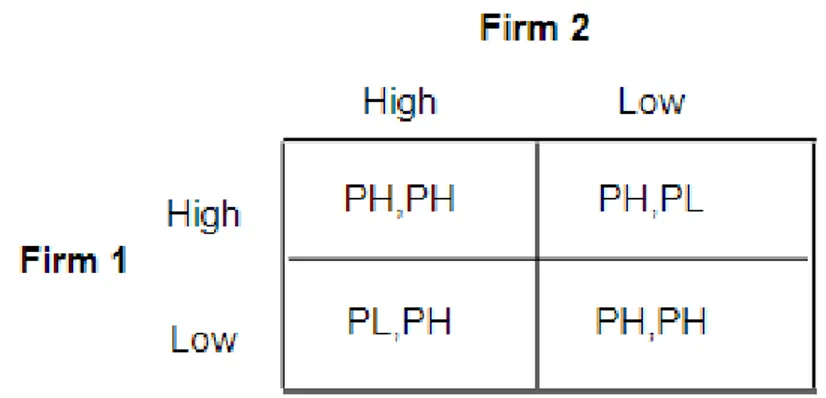
2.4.8 Duopsony game

A duopsony game is a type of two-player two-action game that can have a mixed strategy or pure strategy outcomes. Two companies produce the same product and buy the same kind of raw material. Each company chooses either to offer a low price (PL) for the raw material or a high price (PH). This is shown in figure 6. Every company wants to achieve the highest possible payoff for themself. The payoff outcome is based on what the company chooses to bid and how much of the raw material the company produces and sells [30].

2.4.9 Cases in duopsony games

Different situations can arise in the forest industry raw material market. The first case can be that the companies choose to cooperate in buying the raw material. In such circumstances, companies collectively bid low to push down the price of raw materials. The extra profit can be shared amongst them secretly. Both companies can hide their cooperation by offering different levels of low. In the second case, companies can choose not to cooperate. In such cases, the price of raw materials is high and remains high until one of the companies can no longer survive on the market. After that, the price falls, and the survivor's market power is increased, and the price remains low until a new competition arises. In the third case, none of the companies cooperate because they lack trust for each other or that both are aware that the government might find out about their conspiracy and punish them. Therefore, both companies are better off by agreeing with the law [30].

2.4.10 The expected payoff in a mixed strategy

It is possible to compute expected payoff for each player through combining profit equations (3) with the best response functions to formulate equation (9) and (10). The equations are similar to those described by Mohammadi Limaei and Lohmander [30].

𝐸𝐴= 𝜋𝐴1𝑋𝑌 + 𝜋𝐴2𝑋(1 − 𝑌) + 𝜋𝐴3𝑌(1 − 𝑋) + 𝜋𝐴4(1 − 𝑋)(1 − 𝑌) (9)

𝐸𝐵= 𝜋𝐵1𝑌𝑋 + 𝜋𝐵2𝑌(1 − 𝑋) + 𝜋𝐵3𝑋(1 − 𝑌) + 𝜋𝐵4(1 − 𝑋)(1 − 𝑌) (10)

2.4.11 Expected payoff hypothesis

Assume a game where the players should determine whether to bid high or to bid low. The players will mix strategies if the expected payoffs are the same. Suppose two players in a game that wish to maximize their profits. Player one can bid high with probability p, and player two can bid high with probability q. Assume that player one can bid low with probability 1 – p and player two can bid low with probability 1 – q. Suppose that player one and payer two are indifferent between offering high bid and low bid. If both players sometimes play high and sometime play low as best response, then it exists a p and q such that the expected payoff of playing high and the expected payoff of playing low is the same [31][32][33].

𝐸1(𝐻) = 𝐸1(𝐿) (11)

2.5 Previous research

Cournot, the author of today's theory of competition, such as monopoly and oligopoly, conducted a duopoly model in which the solution is comparable with the Nash equilibrium [34]. Zermelo and Borel demonstrated that if both players in chess use pure strategy, there exists at least one equilibrium outcome [35]. Von Neuman and Morgenstern studied numerous mathematical applications of game theory of different forms with appropriate logic in various fields, such as economic and sociological problems [28]. Nash introduced a new solution concept and is the most commonly used equilibrium state in modern game theory [29]. Borel made the initial efforts in mathematical applications of game strategy in zero-sum, symmetric, restricted two-player games [36].

In recent years, game theory has been applied to investigate competition in the forest industry. Lohmander applied game theory in a two-player non-zero-sum game where each player wants to optimize their profits either through a pure or mixed strategy based on the last observed frequency of the other player's action. A doupsony game is applied between two competing sawmills. The dynamic solution appears to be a circular trajectory [37]. Mohammadi Limaei applied dynamic game theory to investigate sawn wood and pulpwood market under a duopoly assumption between mills in northern Iran. Results indicated that the two competing mills use a mixed strategy in setting product selling prices [38]. Mohammadi Limaei and Lohmander applied dynamic game theory to investigate the timber market as a duopsony assumption between two mills in northern Iran. Results indicated that the two competing mills used mixed strategies in the raw material market when bidding to purchase timber from forest owners [30]. Mohammadi Limaei applied dynamic game theory to investigate the pulpwood market under a duopsony assumption between two mills in northern Iran. Results indicated that the two competing mills use mixed strategies when bidding to purchase the pulpwood from forest owners [39].

3 Method

This chapter describes a method overview, how data has been collected, and how data has been processed, structured, and analyzed. This section describes the mathematical tools and models that have been used to investigate the issues and a brief model discussion.

3.1 Overall method

This paper is based on literature that consists of scientific research, that is, scientific publications, such as papers and articles in scientific journals. The empiricism consists of statements from scientific publications and the company's own annual and interim reports as well as information from websites. The study is grounded on quantitative research, which bases its results on numerical data. The literature search was done with databases such as Google Scholar through carefully selected keywords such as "game theory," "forest industries," "duopsony," and "Nash equilibrium." By combining different keywords, suitable articles were found.

3.2 Excel

Excel was used to structure the data in tables. The regressions were implemented in Microsoft Excel 2019 through one of Excel's inbuilt tools called "data analysis."

3.3 Draw.io

Draw.io was used to create figures and models in order to facilitate understanding of different theoretical parts and to explain how different theories come together through process modeling.

3.4 Data collection

In order to carry out the regression analysis, quantitative data for the regressors were mainly obtained from _{annual reports, interim reports,} presentations, and websites. The data used to measure the market concentration was collected from Sweden's central bureau of statistics (SCB). Bidding price or raw material costs were obtained from a forest association called SKOGEN with over 8600 members who continuously update the forest industry companies' pricelists.

3.5 Selections of variables

This section explains the choice of regressors and how they have been intended to be used in the regression model.

3.5.1 Dependent variable

The main goal for all companies, according to one of the essential theories of the IO "theory of the firms" is to maximize profits. According to economic theory. The profit is measured by taking total revenue minus total costs. In this report, revenue and variable costs have been used as dependent variables to calculate the profit as EBITDA (Earnings before interest, taxes, depreciation, and amortization). Fixed charges have been excluded since it does not have a significant impact on the result in higher sale quantities.

3.5.2 Independent variables

The variables in the model have been selected by considering which factors that affect the revenue and variable costs. The regressors are the product price, raw material price, and product quantity.

3.5.2.1 Product price

The product price indicates the equilibrium price or market clearing price for paper.

3.5.2.2 Raw material price

Raw material price indicates the bids that the companies place to purchase pulpwood from the forest owners.

3.5.2.3 Quantity

Quantity indicates the amount of paper that each company produces from purchased raw material.

3.6 Herfindahl-Hirschman Index

HHI-score was used to identify the company's size in relation to the whole industry through market shares and thus investigate and measure market concentration. This was done by taking the sum of squared market share for all firms in a given market multiplied by 10,000 equation (4). The scores were then demonstrated in a graph showing how the HHI index had varied during a specific time period.

3.7 Regression model

Regression analysis was applied to the retrieved quantitative data taken from the company's reports to identify correlations between the quantitative data and thus develop a linear relationship which was formulated into equations

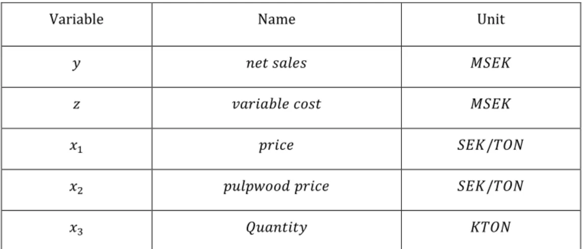
The basic model was based on the inclusion of all defined variables. The model was then evaluated by statistical tests to investigate which variables should be included in the final model. The included variables are shown in table 1.

Table 1: Describes the model variables

Variable Name Unit

𝑦 𝑛𝑒𝑡 𝑠𝑎𝑙𝑒𝑠 𝑀𝑆𝐸𝐾

𝑧 𝑣𝑎𝑟𝑖𝑎𝑏𝑙𝑒 𝑐𝑜𝑠𝑡 𝑀𝑆𝐸𝐾

𝑥1 𝑝𝑟𝑖𝑐𝑒 𝑆𝐸𝐾/𝑇𝑂𝑁

𝑥2 𝑝𝑢𝑙𝑝𝑤𝑜𝑜𝑑 𝑝𝑟𝑖𝑐𝑒 𝑆𝐸𝐾/𝑇𝑂𝑁

𝑥3 𝑄𝑢𝑎𝑛𝑡𝑖𝑡𝑦 𝐾𝑇𝑂𝑁

3.7.1 Formulating the profit equations

According to equation (8) the equation for net sales and the equation for variable cost can be formulated as:

𝑦 = 𝛼0+ 𝛼1∙ 𝑥1+ 𝛼2∙ 𝑥3+ 𝜀1 (15)

𝑧 = 𝛽0+ 𝛽1∙ 𝑥2+ 𝛽2∙ 𝑥3+ 𝜀2 (16) According to equation (3) the profit equation can be formulated as:

3.8 Expected payoff equation and Nash equilibrium

The profit equation (17) can be used to construct the expected payoff equations (9) and (10). Nash equilibrium probabilities in mixed strategy can be determined by derivation of each payoff equation with respect to the probability distribution variables X and Y set to zero and finally solved for X and Y [30]. 𝜕𝐸𝐴

𝜕𝑋 = 𝜋𝐴1𝑌 + 𝜋𝐴2(1 − 𝑌) − 𝜋𝐴3𝑌 − 𝜋𝐴4(1 − 𝑌) = 0 (18) 𝜕𝐸𝐵

𝜕𝑌 = 𝜋𝐵1𝑋 + 𝜋𝐵2(1 − 𝑋) − 𝜋𝐵3𝑋 − 𝜋𝐵4(1 − 𝑋) = 0 (19)

When the Nash equilibrium probability's (N_x, Ny) are calculated, then no player

has further reason to change strategy [30], and the Nash equilibrium expected payoff can be determined through these probabilities.

𝑞 = 𝑁𝑦 𝑤ℎ𝑒𝑟𝑒 𝜕𝐸_𝜕𝑋𝐴= 0 and 𝑝 = 𝑁𝑥 𝑤ℎ𝑒𝑟𝑒 𝜕𝐸_𝜕𝑌𝐵= 0 (20)

3.8.1 Expected payoff hypothesis test

The expected payoff hypothesis can then be tested for indifference by plugging the value of p and q into expected payoff equations (12) and (14). If the p and q contribute to indifference, then the expected payoff is a valid estimation.

3.9 Dynamics of the mixed strategy game

Both players have two possible choices when buying raw material either to bid high or to bid low. The game is about examining what the player's strategic action will be based on what the other is doing. The dynamic game was applied to gain an analytical understanding of the pulpwood market under the assumption that the market structure was characterized as a duopsony. It was assumed that the players did not have complete information. However, the players could observe the frequencies of the decisions made for the other player. This makes the bidding in the raw material market to follow a particular trajectory [30][37].

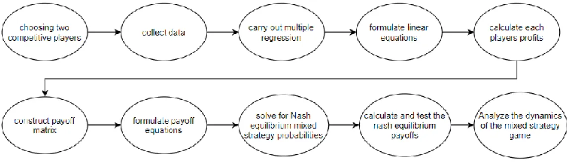
3.10 From data to a Game theory application

A dynamic two-person non-zero-sum game was constructed, which is a repeated game that involves two-player that compete for the payoff. The competition included two companies, player A (SCA) and player B (Holmen). Both players compete against each other to buy raw materials from forest owners and to sell it refined at a product market. The payoff matrix was made by combining Figures 5 and 6 and equation (17).

Each player's profit function is based on equations derived from regressions equations (15)(16)(17). Expected payoff equations (9) and (10) were then formulated based on several profit equations derived through equation (17). The Nash equilibrium probabilities were calculated mathematically through partial derivates of the payoff equations, equation (18) and (19), and the Nash equilibrium expected payoff results were calculated and tested through equation (12) and (14). Finally, the dynamics of the game where analyzed. The whole process is shown in figure 7.

3.11 Method discussion

The ability to criticizing quantitative studies is of great importance. One should not only focus on the final result but also on how well the researches have strived to increase the quality of the study. In quantitative analysis, this may be achieved by measuring validity and reliability. Validity refers to how accurately a particular concept has been measured in quantitative research, and reliability refers to the consistency of a measure [40]. A high validity also implies high reliability because it increases the overall trustworthiness of the study in general.

3.11.1 Reliability

A measurement has high reliability if it produces approximately the results when repeated several times [40]. This study has high reliability because it is based on models that have a proven linear relationship between data, and only the highest correlations are included; thus, a similar study with similar data would give the same results. The study is inspired by the work of Mohammedi Limaei and Lohmanders, and even two other studies carried by only Mohammadi Limaei that have a similar approach; thus, this approach has been tested more than three times before and produced identical results. For example, the mathematically proven movement pattern or trajectory used to analyze the markets are similar to theirs but with different Nash equilibrium values.

3.11.2 Validity

The study is based on several sources that highlight the science of game theory. The game theory concept is based on the book "A course in game

theory" by Osborne and Rubinstein and "theory of games and economic behavior" by Neumann and Morgenstern. Nash equilibrium theory is based

on the book "equilibrium points in n-person games" written by Nash himself. The study as a whole is inspired by a similar scientific publication, "A game theory approach to the Iranian forest industry raw material market" by Mohammadi Limaei and Lohmander, which draws identical conclusions [30]. Primary sources regarding the concepts have been used to strengthen the validation. Hypothesis tests were used to validate the model by looking at the p-value. The P-value for the coefficients less or equal to 0.05 was considered significant. The goodness of fit was also used to validate the model by identifying the coefficient of determination and adjusted coefficient of determination with the highest correlation, i.e., which is closest to 1. The expected payoff hypothesis was formulated to test for indifference to see if the Nash equilibrium probabilities results were valid.

3.12 Ethical and societal aspects

The elementary ethical moralities of every researcher are intellectual uprightness, which must be existing in all phases of scientific work: from theory, methodology, analysis, and explanation of the results [41].

The study uses high-quality data to ensure increased scientific awareness and credibility. The choice of literature, methodology, statistical tests, analysis of the results hold honesty, criticism, and transparency.

What motivated this study from an ethical perspective was the unfair, one-sided prices that can be set by the buyer in the raw material market since the sellers of pulpwood do not have the ability or power to freely determine the price. In a concentrated product market, a similar situation exists, but vice versa. In this case, it is the seller who has the power to put unreasonably high prices on consumers. What also motivated this investigation from a societal perspective was the possibility for cartel formations and cooperative behavior in imperfect markets because it often leads to higher prices and worse product offerings and harms the competition, consumers, and the economy.

4 Results

4.1 SCA regression data

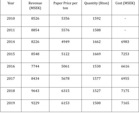
Regression data was gathered from SCA, such as total revenue, the paper price per ton, delivered quantity, and cost of production (Table 2) from SCA interim and annual reports [42].

Table 2: Collected data from SCA

Year Revenue

(MSEK)

Paper Price per ton

Quantity (Kton) Cost (MSEK)

2010 8526 5356 1592 - 2011 8854 5576 1588 - 2014 8226 4949 1662 6983 2015 8548 5122 1669 7253 2016 7744 5061 1530 6616 2017 8434 5678 1577 6955 2018 9643 6315 1527 7175 2019 9229 6153 1500 7165

4.2 Holmen regression data

Required data for regression analysis was gathered from Holmen, such as total revenue, the paper price per ton, delivered quantity, and cost of production (Table 3). Holmen interim and annual reports [43].

Table 3: Collected data from Holmen

Year

Revenue (MSEK)

Paper Price per

ton Quantity (Kton) Cost (MSEK)

2010 8142 4701 1732 7913 2011 8631 5159 1673 7629 2012 8144 4933 1651 7282 2013 7148 4541 1574 6720 2014 6247 4787 1305 5522 2015 6148 4640 1325 5634 2016 5431 4789 1134 4761 2017 5408 4842 1117 4781 2018 5571 5377 1036 4905 2019 5757 5780 996 4866

Required data for regression analysis was gathered from SKOGEN, such as bidding price or raw material costs, and displayed in a graph to show the bidding pattern (Figure 8). SKOGEN [44].

4.3 SKOGEN regression data The bids from 2010 to 2020 (Figure 8).

Figure 8. Collected data from SKOGEN and price bid graph

The price difference (Figure 9) was calculated and displayed in a graph to show deviations.

4.4 Price difference

The price difference between the bids from both companies (Figure 9).

2010 2011 2012 2013 2014 2015 2016 2017 2018 2019 2020 SCA Real Price

Västernorrland 321 357 314 271 272 272 269 264 259 316 296 Holmen Real Price

Hälsingland 309 361 298 271 250 250 248 264 264 326 296 321 357 314 271 272 272 269 _{264 259} 316 296 309 361 298 271 250 250 248 264 264 326 296 0 50 100 150 200 250 300 350 400 SE K

/ton SCA Real Price

Västernorrland Holmen Real Price Hälsingland 12 -4 16 0 22 22 22 0 -5 -10 0 -20 -10 0 10 20 30 2010 2011 2012 2013 2014 2015 2016 2017 2018 2019 2020 SE K /TO N

Required data to measure HHI was gathered from SCB, such as total industry revenue and total industry members. SCB, according to business economics [45].

4.5 Herfindahl-Hirschman data

The Total paper industry revenue and total members of the paper industry are shown in Table 4.

Table 4. Collected SCB data

Year Revenue (MSEK) Number of companies

2010 21 626 335 2011 22 143 329 2012 21 950 329 2013 21 441 320 2014 21 722 303 2015 22 234 289 2016 22 450 288 2017 23 449 282 2018 24 806 285

Graphical representation of the market concentration based on the data from Table 4 is shown in Figure 10. HHI scores have varied over the years. The future prediction is displayed in a trend line.

4.6 Herfindahl-Hirschman Index graph

The HHI-scores over the years are shown in Figure 10.

Figure 10. HHI-scores 0 1000 2000 3000 4000 2010 2011 2014 2015 2016 2017 2018 H H I SCO R E YEAR

Herfindahl-Hirschman Index

4.7 Holmen regression results

The regression results and hypothesis test for Holmen (Table 5) are based on revenue data as a dependent variable and price per ton and quantity as independent variables.

Table 5: Regression results when the dependent variable is revenue and hypothesis test results for Holmen

The goodness of fit results for Holmen based on the same regressions described in Table 5 is shown in Table 6.

Table 6: Goodness of fit test results

Goodness of fit

R-square 0,995536

Adjusted R-square 0,994261

Observations 10

Standard error 94,59642

The regression results and hypothesis test for Holmen (Table 7) are based on production cost data as a dependent variable and pulpwood price per ton and quantity as independent variables.

Table 7: Regression results when the dependent variable is production cost and hypothesis test results for Holmen

The goodness of fit results for Holmen based on the same regressions described in Table 7 is shown in Table 8.

Table 8: Goodness of fit test results

Coefficients P-value

Intercept -5903,34 1,87E-05

Price per ton 1,177384 5,19E-06

Quantity 4,970996 1,99E-09

Coefficient P-value

Intercept -2720,14 1,1E-07

Pulpwood price 10,359711 4,24E-08

Quantity 4,3285536 1,3E-12

Goodness of fit

R-square 0,9994639

Adjusted R-square 0,9993108

4.8 SCA regression results

The regression results and hypothesis test for SCA (Table 9) are based on revenue data as a dependent variable and price per ton and quantity as independent variables.

Table 9: Regression results when the dependent variable is revenue and hypothesis test results for SCA

The goodness of fit results for SCA based on the same regressions described in Table 9 is shown in Table 10.

Table 10: Goodness of fit test results

The regression results and hypothesis test for SCA (Table 11) are based on production cost data as a dependent variable and pulpwood price per ton and quantity as independent variables.

Table 11: Regression results when the dependent variable is production cost and hypothesis test results for SCA

Coefficients P-value

Pulpwood price 9,7545896 0,003222

Quantity 2,8095114 0,000423

The goodness of fit results for SCA based on the same regressions described in Table 11 is shown in Table 12.

Table 12: Goodness of fit test results

Goodness of fit R-square 0,9998073 Adjusted R-square 0,7497591 Observations 6 Standard error 119,49234 Coefficients P-value

Price per ton 1,1122586 0,000177

Quantity 1,5857371 0,015719 Goodness of fit R-square 0,9994159 Adjusted R-square 0,8326519 Observations 8 Standard error 241,90297

4.9 Equations Holmen equation:

Based on the results from Tables 5 and 7, the final equation:

𝜋𝑝= (1,18 ∙ 𝑃𝑠+ 4,97 ∙ 𝑄𝑝 − 5903) − (10,36 ∙ 𝑃𝑝+ 4,33 ∙ 𝑄𝑝− 2720) (21)

SCA equation:

Based on the results from Tables 9 and 11, the final equation:

4.10 Game theory applications

Figure 11 shows the payoff matrix. X equals the probability that SCA goes for a low bid. (1-X) equals the likelihood that SCA goes for High bid. Y equals the likelihood that Holmen goes for a low bid. (1-Y) equals the probability that Holmen goes for the high bid. P_A and P_B is the pulpwood price (SEK per ton), P_s is the paper price (SEK per ton), π is the EBITDA (MSEK), and Q represents the quantity (Kton).

Holmen Low High Y (1-Y) 𝑷𝑨=260 𝑸𝑨=1577 𝑷𝑨= 260 𝑸𝑨=1527 Low X 𝑷𝑩=260 𝑸𝑩=1117 𝑷𝑩=265 𝑸𝑩= 1036 𝑷𝒔=5500 𝑷𝒔= 5500 𝑷𝒔= 5500 𝑷𝒔=5500 SCA 𝝅𝑨=1631 𝝅𝑩=1328 𝝅𝑨=1692 𝝅𝑩=1223 𝑷𝑨=265 𝑸𝑨=1530 𝑷𝑨=265 𝑸𝑨=1500 High (1-X) 𝑷𝑩=260 𝑸𝑩=1134 𝑷𝑩=265 𝑸𝑩=996 𝑷𝒔=5500 𝑷𝒔=5500 𝑷𝒔=5500 𝑷𝒔=5500 𝝅𝑨=1639 𝝅𝑩=1339 𝝅𝑨=1676 𝝅𝑩=1199

Expected payoff and Nash equilibrium

ESCA= 1631XY + 1692X(1 − Y) + 1639Y(1 − X) + 1676(1 − X)(1 − Y) (23) SCA wants to know if it can increase payoff by increasing or decreasing X. ∂ESCA

∂X = 1631Y + 1692(1 − Y) − 1639Y − 1676(1 − Y) = 0 (24) ∂ESCA

∂X = 3𝑌 − 2 = 0 (25)

SCA has no reason to change X if Y = 0.667

EHolmen= 1328YX + 1223Y(1 − X) + 1339X(1 − Y) + 1199(1 − X)(1 − Y) (26)

Holmen want to know if it can increase payoff by increasing or decreasing Y. ∂EHolmen

∂Y = 1328X + 1223(1 − X) − 1339X − 1199(1 − X) = 0 (27) ∂EHolmen

∂Y = 7𝑋 − 4.8 = 0 (28)

Holmen has no reason to change Y if X = 0.686

Ny= 0.667 where ∂E_∂XSCA= 0 and Nx= 0.686 where ∂EHolmen_∂Y = 0 (29) The mixed Nash equilibrium probabilities are Y = 0.667 and for X = 0.686

Expected payoff calculation

𝐸𝑆𝐶𝐴(𝐻) = 𝐸𝑆𝐶𝐴(𝐿) (30)

1631 ∙ 0.667 + 1692 ∙ (1 − 0.667) = 1639 ∙ 0.667 + 1676 ∙ (1 − 0.667)

≈ 1651 𝑀𝑆𝐸𝐾 (31)

The expected payoff for SCA is equal to 1651 MSEK.

𝐸𝐻𝑜𝑙𝑚𝑒𝑛(𝐻) = 𝐸𝐻𝑜𝑙𝑚𝑒𝑛(𝐿) (32)

1328 ∙ 0.686 + 1223 ∙ (1 − 0.686) = 1339 ∙ 0.686 + 1199 ∙ (1 − 0.686)

≈ 1295 𝑀𝑆𝐸𝐾 (33)

Dynamical game theory

Both companies use mixed strategies to choose between low or high bid. Suppose SCA and Holmen are assigned probability X and Y, individually, to select a low offer. The mixed strategy Nash equilibrium is (0.667, 0.686). There is no guarantee that the various companies have complete information about each other, i.e., awareness of each other's costs and revenues. But what both companies can observe are each other's bids in respective price lists.

Each director observes the mixed strategy frequency of the other, and the expected marginal profits could be derived trough (∂ESCA

∂X 𝑎𝑛𝑑

∂EHolmen

∂Y ). In

case the marginal profit of SCA: s mill is strictly positive (zero or purely negative), SCA increases (leaves unchanged, decreases) X. In the case, the marginal profit of Holmen is purely positive (zero or strictly negative), Holmen increases (leaves unchanged, decreases) Y. Based on the assumption that the rate of change of X and Y is proportional to the expected marginal profits, that is, both SCA and Holmen have the same relation between the rate of change and expected marginal profit. Assume that 𝐶1 𝑎𝑛𝑑 𝐶2 is the rate of change for SCA and Holmen respectively and that

𝐶1 = 𝐶2 [30][37].

Equation (25) can be re-expressed as:

𝑋̈ = 𝐶1∙ ∂EA

∂X (34)

or 𝑋̈ = 𝐶1∙ (3𝑌 − 2) (35)

Equation (28) can be re-expressed as:

𝑌̈ = 𝐶2∙ ∂EB

∂Y (36)

Or 𝑌̈ = 𝐶2∙ (7𝑋 − 4.8) (37)

This gives the resulting mixed strategy trajectories in Figure 12, which shows the trajectories repeatedly looping from the region a to d with the Nash equilibrium at the center. Mohammadi Limaei and Lohmander show the mathematical dynamical framework and proof of this mixed strategy trajectory [30].

Figure 12. Mixed strategy trajectory

Region a: X>0.686, Y<0.667. Holmen often give low bids, and SCA often

offers high bids. As Holmen often gives low bids, SCA finds it profitable also to bid low, so SCA decides to bid low more often; thus, the system moves to region b.

Region b: X>0.686, Y>0.667. Both companies give low bids. Holmen

understands that it may be more profitable to bid high more often, thus Holmen bids high and the system movies to region C.

Region c: X<0.686, Y>0.667. Holmen often give high bids, and SCA often

offers low bids. SCA finds it profitable to go for high binds more often; thus, the system moves to region d.

Region d: X<0.686, Y<0.667. Both companies give high bids. Holmen finds

it profitable to give low bids more often; thus, the system once again moves to the region a.

5 Discussion

This chapter talks about SCA and Holmen's regional competition for raw materials and the HHI results. It also talks about the regression results, the equation development and discusses the dynamic duopsony game.

Competition in the pulpwood market

We look at Porter's five forces when analyzing competition in the paper industry. These five forces are sellers' market power, buyers' market power, whether it is easy for newcomers to enter an industry, and if there are threats from substitutes. That is, products that can offer a better solution and replace the existing products. This study focuses on two of these five forces. It is buyer and seller market power, but we will discuss all forces in this part.

In a non-competitive market, there may exist market concentration either on the buyer side (demand side) or on the seller side (supply side). If the buyer side is concentrated, then we say that the buyer has market power, and if the seller side is focused, we assume that the seller has market power (Figure 4). Market power means that a buyer or a seller can adapt the market to increase their benefits. If a company has both buyer power and seller power, then they can exploit the imbalance in the market by buying cheap and selling expensive. This process is called arbitrage [1]. Companies with a lot of strength can shape cartels by cooperating. It means that they can together take full control over a market. In the supply-side companies can dominate what should sell, how much should sell, and at what price to sell it. Looking at the demand side, companies can dominate what to buy, how much to buy, and at what cost to buy it. We say they act in unison to get monopoly or monopsony power. If a company has power in raw material and has power on a product market, then it can have both monopolistic and a monopsonistic power at the same time [17][20]. It is a dream condition or the ultimate state for businesses. In reality, if we look, for example, in the raw material markets, different outcomes can occur. One case is that companies cooperate, thus buying the raw materials cheaply by offering low prices. In other cases, companies can choose not to work together, then one company offers a higher bid than the other, thus forcing the other to bid high as well [30]. We look deeper into this when analyzing the dynamics of the pulpwood market through dynamical game theory.

We are investigating the competition in the pulpwood market and the paper market as we know that SCA and Holmen are two large companies in the paper industry that refines pulpwood. We know that both SCA and Holmen each month submit a price list, which includes biddings for pulpwood. The

should cost. If they did not have such authority, then the forest owners would instead be the ones to put a price for what they want in payment for their raw materials like in a normal competitive market. This statement reinforces our assumption that the pulpwood market is concentrated. We assume that it is a duopsony by the selection of two areas in Sweden that Holmen and SCA have strong buyer influence in (Va sternorrland and Ha lsingland). It leaves us to ponder how concentrated the paper market is. In response to this, we use the HHI method. An HHI between 1,500 and 2,500 represents a reasonably focused market. An HHI over 2,500 means that the market is concentrated for sure. The results showed that HHI varies between 3100 and 1700. It indicates that the paper market is highly concentrated, but over time, it has begun to become less concentrated (Figure 10). The paper market is slowly going from being non-competitive to becoming more competitive. While HHI has declined over the years, the number of companies in the paper industry has also declined (Table 4). The threat from new entrants cannot be behind why the paper market is moving towards a competitive market and the reason why SCA and Holmen are losing their monopolistic power. The only logical answer is that the whole industry's revenue is becoming more evenly distributed over time to already existing members of the industry. Threats from substitutes are also not believed to be behind the reduction in the market concentration since we can see that deliveries of paper have gradually decreased each year. One theory is that digitalization is behind the decrease as magazines and newspapers have become increasingly electronic over the years, e.g., because of social media, etc. Another factor that we believe had influenced the HHI value is the split that took place in 2017 when SCA was divided into two companies [46].

Regression analysis

We use regression analysis to produce correlations between data obtained from annual reports and interim reports and other data sources. Through these relationships, we created multivariable profit equations that can give realistic EBITDA values.

Under the regression analysis, we tested all regressors to increase the validity of the model. Only the variables with a p-value below 0.05 were added to the model.

For Holmen, the intercept was also included because it gave a better p-value and a higher adjusted coefficient of determination (R-square). The goodness

For SCA, the intercept was not added. Because excluding the intercept gave better p-value and higher R-square. The goodness of fit of the first regression yielded 83% R-square, and the second regression yielded 75%, which is acceptable. The first regression was based on eight observations and had a high standard error, and the second regression was based on six observations and had a better standard error. SCA did not give the same precision compared to Holmen. It is because annual reports and interim reports for some years lacked clear information about revenue and costs. Game theory analysis

The payoff matrix became a two-person non-zero-sum game that analyses the event between 2017 and 2019. We used the actual quantities for these years. However, SCA had a higher selling price on paper than Holmen. The reason behind this is that SCA considers kraft liner to be a paper product, and because kraft liner is a bit thicker than standard paper, the price will be higher. An average value (5500 SEK per ton) was calculated to minimize the price difference that comes from kraft liner.

In 2017 there was no price difference for pulpwood between Holmen and SCA. In 2018 however, the difference was 5 SEK per ton, and in 2019 the difference was 10 (Figure 9). We took the average difference between 2017 and 2019, which gave us 5. Thus, we chose to vary the price of pulpwood by 5 (the low cost of 260 SEK and high cost 265 SEK) in the payoff matrix (Figure 11).

We could assume that the players were using a mixed strategy because both companies bid high sometimes and low sometimes. We could also assume that the bidding followed a trajectory because the prices showed a repeating pattern (Figure 8). An attempt was made to find a Nash equilibrium because Nash claimed that there always existed an equilibrium in a mixed strategy game [29]. It was done through partial derivatives of the expected payoff equations (equations 25 and 28). When the probabilities that made neither Holmen nor SCA interested in changing their strategy were derived, we realized that there existed a Nash equilibrium. To verify that these probabilities were actual equilibrium probabilities, we inputted them in a simplified equation (equations 31 and 33) to test whether these probabilities made the companies indifferent between choices of strategy. The result showed indifference when the expected payoff for SCA is 1651 MSEK, and the expected payoff for Holmen is 1295 MSEK.

Finally, we used dynamic game theory to analyze the dynamics of the game as the players use mixed strategies and to describe the cases when the Nash equilibrium is not reached. We followed Mohammadi Limaei and