Relationship
between
Real
Estate Industry and Stock
Market in China
MASTER
THESIS WITHIN: Economics NUMBER OF CREDITS: 30
PROGRAMME OF STUDY: Economic analysis AUTHOR: Zeyu Di
Master Thesis in Economics
Title: Relationship between Real Estate Industry and Stock Market in China Authors: Zeyu Di
Tutor: Almas Heshmati Date: 2020.05.18
Keywords: real estate; stock market; causal relationship; asset allocation; economic area; portfolio; Chinese provinces
Abstract
Each individual is both a consumer and an investor in the market. It is the common goal of every investor to achieve a high return on investment through the portfolio of profit maximization. As a result, the ratio of assets in a portfolio has become a hot topic. In China, real estate and the stock market are two main markets favoured by both individual and institutional investors. And there is a significant economic link between the two markets. Therefore, their mutual relationship and long-term and short-term causality can provide good guidance for investors. This paper studies the causality and correlation between stock trading volume and real estate trading volume in 31 provinces of mainland China. The empirical results in this paper is based on a panel data from 2000 to 2016 and divides 31 provinces into three different economic regions. The panel unit root test and the Pedroni co-integration test were carried out. The Hausman test was used to select among different estimation methods. Panel Mean Group is found the most suitable analysis method. It is found that the main industries in different provinces may affect the short-term causal relationship between real estate and the stock market. But in the long run, the causal relationship between real estate and the stock market is two-way and stable.
Table of contents
1. Background of real estate and stock market in China ... 1
2. Introduction ... 3
3. Literature review ... 5
3.1 Theories related to housing-stock market relationship ... 5
3.2 Empirical studies of housing-stock market relationship ... 7
3.2.1 Research suggesting stocks will affect real estate ... 7
3.2.2 Research suggesting real estate will affect stocks ... 9
3.2.3 Evidence of long-term equilibrium and two-way causality relationship ... 9
3.2.4 The influence of "special time" factor on housing-stock market relationship ... 11
4. Data and description of variables ... 13
5. Methodology ... 17
6. Estimation Procedure... 20
6.1 Descriptive statistics ... 20
6.2 Correlation test ... 20
6.3 Panel autoregressive distributed lag (ARDL) estimation method ... 21
5.4 Discussion of the estimation result ... 26
7. Conclusion and Recommendations ... 27
7.1 Summary and recommendations ... 27
7.2 Limitation of this study and suggestions for future research direction ... 28
References ... 31
Appendix ... 34
List of appendix tables Table 1 Definition of all the variables ... 34
Table 2 Descriptive statistics of key variables over time ... 35
Table 3 Pearson correlation coefficient matrix of all variables ... 36
Table 4 Summary of the optimal lag of all the variables for different provinces .... 37
Table 5 The result of Pedroni cointegration test ... 38
Table 6 Summary of 3 different estimation method and Hausman test ... 39
Table 7 Causal relationship in the short-run between real estate and stock market in 31 provinces of China ... 40
List of Figures
Figure 1 Summary of literature on the relationship between real estate and stock market ... 12 Figure 2. Summary statistics of main variables and control variables, 2000-2016
... 16
List of Abbreviations
CHSOR Commercial housing sales
NSR Aggregate stock market for domestic investors INSR Aggregate stock market for international investors GDP Gross Domestic Product
RGDP Real GDP. The value calculated by the nominal GDP and the GDP deflator GDPPC GDP per capita
This thesis investigates the relationship between stock market and real estate market in different provinces in China by studying the influence of transaction amounts in different stock markets on comprehensive commodity housing prices. According to Liow (2006), both the stock market and real estate are very important components for the country. The stock market shows the economic situation of enterprises and listed companies, as well as the investment demand of investors, with stock indexes and trading transactions. For both companies and individuals, real estate is an indispensable and rigid asset. Liow also notes that when the economy is booming, the benefits to companies and manufacturers can lead to a boom in the stock market. With the supply and demand ratio unchanged, real estate prices will rise accordingly. Therefore, there may be a long-term or short-term relationship between the stock market and the real estate market.
1. Background of real estate and stock market in China
In China, commercial housing is not only one of citizens’ rigid demand, but also the commodity property of real estate is infinitely magnified (China building industry press, 2009). Also, a considerable number of citizens have commercial housing as the first choice for investment. However, as a traditional investment choice, stocks are still one of the most popular investment markets (Wang, 2015). He also mentioned that real estate and stocks are two economic commodities held by most Chinese households. In other words, portfolios of stocks and real estate are extremely popular in China. For individuals, we can freely allocate funds between real estate and the stock market. For companies, especially public corporates, they hold both property and shares. According to Chen, Han and Wu (2012), the net profit of enterprises, stock market value and real estate prices also have a mutual influencing relationship. At the national level, the Chinese government formulate corresponding monetary policies to conduct control on the stock market and real estate (Guo et al., 2013). Because the monetary policy will affect the real estate and stock market through the reserve requirement ratio. Therefore, the stock market and real estate, as two major sectors in the economy, may interact directly or indirectly.
The property market has been an important part of China's economy. Glaeser and Gyourko (2005) investigated the Chinese real estate market under the "reform and opening up" policy between 1970 and 2000. During this period the housing prices in some coastal cities had soared; but for the rest of China, such as the western and middle area,
the prices are lower, and supply is plentiful. Since the beginning of the 20th century, China's economy has entered an era of rapid development. At the same time, the real estate industry is developing particularly fast. Since 2003, the value of China's real estate has increased tenfold, contributing 6.87% of China's GDP in 2018 (CEIC, 2020). Real estate market is a comprehensive market, it contains raw materials, tangible capital and intangible capital. Therefore, the real estate market is thriving so much because of the development and help from other industries and other fields.
China's real estate market is fundamentally different from that of western countries. According to Glaeser et al. (2017), the real estate market of China has the characteristics of high vacancy rates, and the ownership of land belongs to the government. Individuals are only allowed to own a home for 70 years, and since the policy was enacted and implemented less than that, it is unclear whether the government will reclaim the right to use the land when it expires. But the government's policy on real estate development since 2003 has not stopped, especially in coastal cities where the real estate market has been flourishing. Fang, Gu, Xiong and Zhou (2015) pointed out that in the second decade of 2003, the average annual growth rate of housing prices in 40 major Chinese cities was 13%, while the net price of land increased fivefold during this period.
In the same way, the stock market in China also had a remarkable development directly from 2000 to 2020, but compared with the real estate market, it was not smooth. According to Trading Economics (2020), China's stock market reached its peak nearly 20 years ago in 2007 and fluctuated periodically in the following decade. The stock market in China is a comprehensive and complex system. According to Kang, Liu and Ni (2002), the investment behaviour of individuals and institutional investors will affect the price fluctuation of the stock market. In that case, Chinese investors' expectations of the stock market are still rising year by year. In addition, Chinese stock market capitalization of GDP growing from 3.93% in 1992 to 36.98% in 2003 (Wong, 2006). The capitalization of the stock market has been accelerating. Wong also claimed that Chinese stock market is characterized by its use as a financing vehicle for state-owned enterprises under undisclosed financial controls. At the same time, the rights and interests of shareholders cannot be fully protected. But even so, citizens and institutional investors are more likely to put 'hot money' into stocks.
2. Introduction
There are 31 provinces and municipalities in China, and which have different level of development and dominant industry. But, obviously, the economy of every province and municipality is affected by the stock and real estate markets. Therefore, it is very interesting to see whether the same relationship between real estate and the stock market can be observed in the case of such differences in research samples. Under such differences, the long-term or short-term relationship between houses and stocks may be regionalized, so the same long-term or short-term relationship is likely to emerge in a certain region of China inducing the need for different state policies. In addition, this thesis will mention two different stock markets, one for domestic investors and one for foreign investors. The two stock markets are not exactly the same in trade of volume, market power, and company type. And the investment cycle of international investors is generally longer than that of domestic investors. Therefore, the impact of the two stock markets on the real estate market is different.
Some previous research focused on the relationship between financial leverage and real estate market in China (Liu and Lei, 2017). There are also studies of housing price movements based on real estate stock prices. For instance, Yang (2005) conducted a research based on the housing price and the price of real estate stocks in Sweden and found a long-term equilibrium relationship between those two. However, Okunev, Wilson and Zurbruegg (2002) devoted to the relationship between the Australian real estate market and the stock market. They found that the fluctuation of stock price would cause the fluctuation of real estate price, and the influence was "rapid". Liow (2006) used the Autoregressive Distributed Lag (ARDL) model to study the dynamic relationship between the real estate market and the stock market in Singapore. Liow found that the real estate market would affect the stock market in the long run, but in the short run, the fluctuation of the stock market would significantly affect the real estate market. However, few literatures have studied countries by region, and few have introduced indicators of other industries as control variables in the specified model. It is possible to overestimate the impact of the stock market on real estate. China is a policy-oriented country and markets can be less responsive to the economy. This means that governments can achieve much better economic results than the market itself, by providing incentives in a given
region or at a given time. In other words, in China, good news and good products in the market are largely related to government policies, rather than the market itself. Even regions with the same level of economic development may react differently to the economy under the influence of policies. Hence, in order to allow to capture heterogeneity in effects, this paper will divide China into three economic areas: eastern, middle and western, expecting to see different relationships between real estate markets and stocks in different regions. Furthermore, this paper will introduce new control variables, such as the number of medical institutions, consumption level and foreign exchange income from tourism and so on, which may influence local housing prices.
The purpose of this thesis is to explore the relationship between the real estate market and the stock market in different provinces (and municipalities) of China. As mentioned earlier, stocks and real estate contribute a significant portion of China's gross domestic product (GDP), and there is a long-term equilibrium between them. Whether this holds true for all provinces, however, is unclear. Some Chinese scholars point out that the stock market affects the price of real estate in the short run, while the price of real estate affects the value of the stock market in the long-term at the national level. But for different provinces, this correlation should not be universal. Therefore, this paper will focus on exploring different relationships in different provinces and expect to find more interesting and heterogeneous connections from the same relationships. For instance, provinces with the same conclusion may come from different economic regions; or these provinces have the same major industries.
This thesis will integrate the methods and viewpoints of previous relevant literatures as the theoretical basis, and on this basis, explore and study the relationship between the real estate market and the stock market. The real estate market and the stock market are two mature and highly developed markets. The autoregressive distributed lag (ARDL) method in the dynamic heterogeneity panel will be used to explore the house-stock relationship. In this paper, while exploring the correlation relationship between the two markets, it is possible to observe that the real estate market has predictive capability over the stock market, and vice versa.
Rest of this research is outlined as follows: the second section will contain literature review and theoretical basis, and the third section will include methodology. This is
followed by a description of the data and a correlation test, with a brief overview of the reasons for selecting these variables. Then for the empirical research section, including results and analysis. The last part is the conclusion. The potential limitations and pitfalls of this thesis are also mentioned before the conclusion.
3. Literature review
3.1 Theories related to housing-stock market relationship
Since there are relatively few literatures on the housing-stock relationship in different regions of a country, this part tries to start from the starting point of how the real estate market and the stock market establish the economic relationship. Markowitz (1959) believed that the portfolio included all types of asset sets held by investors. This collection of assets should include not only a variety of securities, but also assets or items with investment attributes. As a result, stocks and fixed assets can make some form of portfolio that can be held by investors. Markowitz also pointed out that according to the "rational economic individual" hypothesis, the goal of capital asset portfolio model (CAPM) is to minimize risks while maximizing returns. The ratio of assets in a portfolio is therefore not static, but a dynamic process.
This paper holds that real estate and stocks are two special commodities with investment attributes, with different nominal prices. The substitution effect works when their relative returns change. Mankiw (2020) mentioned in his latest edition of the book that the change of commodity price may influence consumers to choose to buy similar goods, and the substitution effect will prompt consumers to make the behaviour of profit maximization. Therefore, for investors whose main goal is to maximize returns, funds will flow freely between the two markets; and investors are more inclined to invest their funds in the market with higher yields. Similarly, Lin et al. (2011) studied the housing-stock relationship of six different Asian economies, and they believed that these two investment methods were mutually substituted.
Keynes (2018) mentioned the wealth effect, pointing out that wealth has a great variety of types, but currency is one of the most important forms. At the same time, his monetary theory included several types of tradable financial assets, such as stocks and bonds.
Keynes thought that the change of wealth is directly reflected in the change of currency, which will affect the investment portfolio of investors and the consumption behaviour of consumers in a short term. Therefore, when investors hold both financial asset investment and fixed asset investment, there is mutual influence between those two.
Kiyotaki and Moore (1997) studied the respective roles of real estate assets and stock assets in the credit process and proposed the theory of credit expansion effect. In their point of view, real estate and stocks can be accepted as collateral in the loan process by various financial institutions, so that these institutions can adjust the amount of loans by the value of the mortgage assets. When stock prices or property prices rise, the total assets of borrowers holding these assets increase, reducing the risk of loans. Therefore, when they apply for a loan, the financial institution will give them more. When a loan is granted, the borrower's cash flow increases, and some assets may be invested in the stock market and the real estate market, which in turn may lead to a potential increase in the price of both assets. Thus, the credit expansion effect provides an explanation for the alternating rise and fall of real estate and stock prices.
From a macroeconomic perspective, the stock and real estate markets are linked by other macroeconomic factors, such as monetary policy, inflation and interest rates. According to Ba, Tan and Zhu (2009), on the premise of free capital flow, real estate and stocks are highly complementary. The real estate volatility is relatively small but the liquidity is low, on the contrary, the stock price volatility is large but the liquidity is strong. They point out that, provided the money supply is adequate and capital flows freely, the return on capital invested in different sectors should be close to the same. As a result, holders of capital withdraw from low-yielding investments and consider investing in higher-yielding investments. It is worth noting that due to the high value and low liquidity of real estate, it is difficult for investors to withdraw capital in time and allocate to the stock market. However, there are few barriers to exit in equities compared with real estate. Therefore, Ba et al. (2009) believes that the adjustment of the stock market to the housing market should be relatively rapid, while the impact of the housing market on the stock market has a long-time lag.
3.2 Empirical studies of housing-stock market relationship
At present, the academic circle has no clear standard on how to study the relationship between the real estate market and the stock market. Most scholars use time series methods for analysis, such as vector autoregression (VAR), and study whether there is a cointegration relationship between them. There are also some researches based on panel data, using fixed effects model or random effect model to study the interaction between the two; or use the dynamic heterogeneity panel and error correction model (ECM) to study the causal and long/short term relationships between those two. In addition, several researchers use nonlinear models to analyse the relationship between the two markets. However, different analytical methods do not lead to completely different conclusions. For some countries, there is a long-term and two-way interaction between housing and equity; in others, the estimated relationship is short-term and one-way.
3.2.1 Research suggesting stocks will affect real estate
First of all, the results of a considerable number of researchers show that stock prices will affect real estate prices. Fluctuations in stock prices can lead to fluctuations in real estate prices. This view is referred to in this article as the "conventional wisdom". The research of Gyourko and Keim (1992), covering the first quarter of 1978 to the fourth quarter of 1990, analysed the risks and returns of real estate companies in two different stock exchanges (New York Stock Exchange NYSE and American Stock Exchange AMEX) in the United States. They argue that estimating the value of real estate is more complicated and a lengthy process than the stock market. However, when real estate companies are securitized, different types of listed real estate companies will react more quickly to changes in stock prices. Their research does not clearly point out the long-term or short-term relationship between housing and stock, but they claim that the real estate market price is significantly affected by the change of stock index, while the real estate price has a very limited impact on stock knowledge.
Similarly, Chen (2001) used bivariate VAR model and multivariate VAR estimation to analyse the real estate and stock market of Taiwan between 1973 and 1992. Chen believes there is a correlation between the price fluctuations of these two assets and that their prices may be related to bank loans and central bank interest rates. But what can be directly
observed is that in this stage, the stock price will significantly affect the real estate price in Taiwan.
In addition, Green (2002) mentioned that the fluctuations of the stock market may affect the real estate market from the perspective of consumption. Green (2002) used the home price index and the Russell index1 from several American cities to represent the housing market and the stock market, respectively, and conducted a simple Granger causality test. He argues that the wealth effect of the stock market varies widely among the U.S. cities. So there is no general correlation between stocks and real estate. But to be sure, stock prices have a positive effect on real estate prices in northern California. It is worth noting that both the studies of Chen (2001) and Green (2002) focus on a specific region. Therefore, their conclusions may not apply to the real estate and stock markets of the whole country, but they are still of reference value.
Okunev et al. (2002) not only fully caters to the traditional views, but also complements them. By analysing the real estate and stock markets in Australia between 1980 and 1999, they found that real estate and stocks do not necessarily influence each other, but there is a one-way causal relationship. When the linear causality test is used, the price change of the stock market will affect the real estate price. When the nonlinear causality test is used, the stock market will still affect the real estate market in a one-way way.
Furthermore, Yang (2005) analysed the monthly data of Swedish real estate market and stock market from 1980 to 1998 by establishing ECM model, and concluded that there was a cointegration relationship between those markets. In fact, the period is in the main real estate cycle, real estate prices are rising trend is quite obvious. Therefore, Yang chose the real estate price index to represent the real estate market, and the stock index to describe the stock market. It is worth noting that due to the small sample size of this study, Yang added a constant trend rather than a time trend to the VAR model. Finally, he points out that the real estate and the stock market show a long-term equilibrium relationship, and the stock price has an indicative effect on the real estate investors.
1 The Russell 2000 Index is a small-cap stock market index of the smallest 2,000 stocks in the Russell
3.2.2 Research suggesting real estate will affect stocks
Shen and Lu (2008) believes that there is a close relationship between the price of real estate and the violent fluctuations of stock prices in China. They used the Johnsen cointegration test, the analysis of variance, and the Granger causality test to empirically study the Chinese stock market and real estate market. They found that between 1998 and 2007, the increase in real estate prices had a significant effect on the rise in stock prices, while the increase in stock prices had a slight effect on the rise in real estate prices. There is a gap of about two quarters between the rise of real estate price and the increase of stock price. Therefore, it can be considered that in mainland China, the mutual influence of stock and real estate exists, but the lag period is long.
According to Lu and Dong (2017), both the real estate market and the stock market are playing an essential role in economic development of China, and there is a certain correlation between price fluctuations and stock price fluctuations. They started from whether the policy can be implemented or not, divided the stages according to the intensity of real estate regulation policies, constructed VAR model for each stage, and conducted comparative analysis of Granger causality test, impulse response and variance decomposition. Lu and Dong believes that although changes in stock prices play a leading role in the causal relationship between the two, the impact of housing prices on stock prices is more significant.
3.2.3 Evidence of long-term equilibrium and two-way causality relationship
However, there might be also a two-way causality or long-term equilibrium between real estate and the stock market. In different countries and regions, the relationship between those two markets may be different. Even in same country or area, different time can present different housing-stock relationship. So the relationship between the two markets is dynamic. According to Stone and Ziemba (1993), Japanese real estate prices peaked in 1991 and accounted for almost 20% of global wealth. Similarly, Japanese stock market peaked in 1989. But by early 1992, Japanese stock market was down 60 percent and land prices were falling rapidly. There are similar and violent fluctuations between real estate and stocks. Stone et al. (1993) selected the land price index and stock index of Japan from 1950 to 1980 and analysed this period of steady development. In Japan, they argue, there is a consistent trend between the two markets, and the stock market lags behind the
property market. This finding contradicts the traditional conclusion that stocks affect house prices in the short term.
In addition, Quan and Titman (1997) reached a conclusion similar to that of Stone et al. (1993). Quan and Titman argues that previous research on the relationship between real estate and the stock market has underestimated the volatility of real estate prices by relying too much on time series models. In their study, they used a single regression method to analyse stock and property data from 17 countries between 1977 and 1994. The study pointed out that there was no correlation between real estate and equities in the United States, Australia or Canada during this period. This conclusion contradicts most research. In some countries, however, the relationship between equity returns and fixed asset rents is significant, then affecting property prices. However, the coefficient of the variable representing commercial housing is significant in all the 17 countries, so there is a correlation in the same direction between real estate and stocks.
The same direction of movement between real estate and equities also applies to the American market. According to Jud and Winkler (2002), based on the American residential price and the S&P 500 index, they used the fixed-effect model to analyse the two variables. In fact, the fluctuation of house prices is not only related to the fluctuation of stock prices, but also affected by other factors, such as population and construction cost. But what is certain is that the boom in the stock market will be a powerful boon to the property market, and that the wealth effect will lag. Jud and Winkler believe that the real estate market will change in the same direction with the change of stock index, and there is a long-term equilibrium relationship between those two markets.
Furthermore, Green (2002) referred to the variable selection method of Jud and Winkler (2002), and he added the new variable of Nasdaq index to optimize the original model. Through Granger causality test, Green found that the real estate market and the stock market showed the same fluctuation trend, and the stock index played a leading role in the relationship. In other words, the stock index Granger cause of the change in real estate prices, whereas real estate prices does not Granger cause the stock index.
Interestingly, Chiang and Lee's (2002) research opened up new ideas for the research of real estate and stock market. Chiang and Lee (2002) chose real estate trust fund instead of real estate price as one of the traditional main variables. They selected monthly data
from real estate funds and stock indexes from 1975 to 1997 and used the return-based style analysis, which is a non-quantitative method. They argue that real estate and fixed assets are viable investments when they are not securitised, but they take a long time to pay off. But it is undeniable that there is a strong correlation between real estate and stocks.
Shun (2004) further explored the relationship between real estate and stocks. He thinks that as a part of the financial market, the stock market has an interaction with the real estate, which indirectly establishes a relationship with the stock market. Shun (2004) selected the monthly data of real estate prices and financial markets in mainland China from 1997 to 2003 for quantitative analysis and established an error correction model between the two markets. Shun pointed out that Chinese real estate market and financial market have a significant two-way causal relationship in both the long and short term. But real estate is less volatile than financial markets. He offers a novel idea: Chinese financial markets are particularly keen on the property market, and the market's huge market capitalisation requires a lot of financial capital. Therefore, China's real estate market and financial market are "inseparable" to some extent.
3.2.4 The influence of "special time" factor on housing-stock market relationship
Moreover, a novel idea has emerged in recent years that "special times" may affect the interaction between real estate and the stock market. Special times can be political or financial, such as the timing of policy announcements or the onset of financial crises. Hui and Ng (2012) studied the long-term and short-term relationship between the housing market and the stock market in Hong Kong from 1990 to 2006. They used the Granger causality test to test the relationship between real estate prices and stock indexes. In fact, the market is volatile during this period. Since Hong Kong transferred sovereignty in 1997, its economy will be strongly affected by the economic fluctuations in mainland China after 1997. Hui and Ng claims that the correlation between stocks and real estate is strong but has weakened over the period and cause and effect has shifted in Hong Kong. Stocks initially affect the price of real estate, but later cannot explain the change in real estate prices through stocks. As a result, the relationship between real estate and stocks is not static, and even within the same region the correlation changes. The connection and Granger causality between them are a dynamic process.
Similarly, Nicholas and Scherbina (2013) studied the relatively early stage development of real estate market and stock market, and they selected the real estate in Manhattan of New York City from 1920 to 1939 for analysis. They believe that the correlation between high-value real estate and stock prices is significant, but the price of ordinary real estate and stock prices are even in the opposite direction. Especially after the 1933 financial crisis, there was no correlation or cause and effect between stocks and real estate. The finding is a challenge to conventional wisdom. But because the range is so old, their conclusions may not apply to the housing and stock markets of recent years. Economic globalization in recent years has allowed investors to freely invest their capital in international markets, rather than in a specific region. This economic network covers more and more countries, which is quite different from 1933. In addition, the ratio of high-value to low-value properties in recent years has changed sharply from 1933. In recent years, Yang and Liu (2015) selected the Gulf Corporation Council – Gneralized Autoregressive Conditional Heteroscedasticity (GCC-GARCH) model to study the dynamic relationship and spillover effect between Hong Kong real estate index and stock index. They argue that the correlation between Hong Kong's property and stock markets reached a high level during the financial crisis, when the two markets moved in the same direction. But in a boom, changes in the stock market can take up to three weeks to feed through to the housing market. In a word, the real estate market in Hong Kong has no significant spillover effect on the stock market, while the stock market will have positive or negative effects on the real estate market in different economic environments.
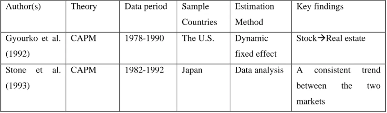
Table 1 provides a summary of the literature on the relationship between real estate and stock markets and findings about the two markets causal relationships.
Figure 1 Summary of literature on the relationship between real estate and stock market
Author(s) Theory Data period Sample Countries Estimation Method Key findings Gyourko et al. (1992)
CAPM 1978-1990 The U.S. Dynamic fixed effect
Stock→Real estate Stone et al.
(1993)
CAPM 1982-1992 Japan Data analysis A consistent trend between the two markets
Quan et al. (1997) CAPM & Wealth effect 1977-1994 17 countries Time-series test (OLS) Stock→Real estate Chen (2001) Rational bubble theory 1973-1992 Taiwan Bivariate VAR Stock→Real estate Green (2002) Wealth effect
1989-1998 The U.S. Granger causality test
Stock→Real estate Chiang et al.
(2002)
CAPM 1975-1997 The U.S. Fixed effect Stock→Real estate Jud et al.
(2002)
Wealth effect
1984-1998 The U.S. Fixed effect Stock→Real estate Okunev et al.
(2002)
CAPM 1980-1999 Australia Bivarite VAR Stock→Real estate Shun (2004) Substitution effect 1997-2003 China Error correction model Stock→Real estate
Yang (2005) CAPM 1980-1998 Sweden ECM Cointegration relationship Shen et al. (2008) Wealth effect 1998-2007 China Granger causality test
Real estate →Stock market Hui et al. (2012) Wealth effect 1990-2006 Hongkong Granger causality test
“Special time” will change the causality Nicholas et al.
(2013)
CAPM 1920-1939 New York VEC Causality depends on real estate prices Yang et al.
(2015)
CAPM 1998-2012 Hongkong GARCH Lag effect
Lu et al. (2017) CAPM 2005-2016 China VAR Real estate →Stock market
4. Data and description of variables
The main research scope of this paper is from 2000 to 2016, a total of 17 years. This time period contains the main part of the rapid development of China's real estate market and stock market. For example, the housing market boomed after 2008, and the stock market boomed in 2015. Furthermore, this period covers before and after the global economic
crisis. The data in this paper cover the population of 31 different provinces and municipalities, and all of them are observed on an annual basis. Therefore, each variable contains 527 annual data points. The data are from the China Stock Market & Accounting Research (CSMAR) database and the national bureau of statistics of China (NBSC). All monetarily measured indicators used in this paper are converted from nominal to real values, based on the price index (2015).
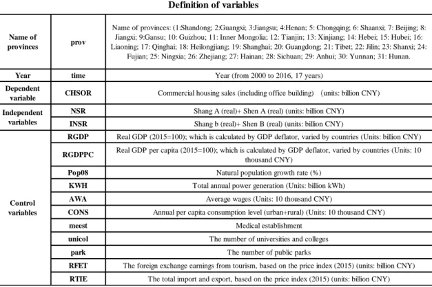
The main variables in this paper are CHSOR, NSR and INSR, which respectively represent the housing price, the stock market that can be invested by domestic investors, and the stock market for foreign investors. Housing prices (CHSOR) are measured by the total number of sales of commercial housing, which includes both office and residential buildings. The data of the stock market is represented by the annual transaction of the stock market, which respectively includes four different stock markets of Shanghai A, Shanghai B, Shenzhen A and Shenzhen B. Since A-shares are only for domestic citizens to invest in and B-shares are only for foreign investors to trade, this paper classifies the stock data into two different parts: national stock (NSR) and international stock (INSR). Secondly, since each province has its own real estate market but it is impossible for provinces or autonomous regions to have their own independent stock markets, this paper uses share of provinces GDP to obtain province-specific stock market turnover, and the data obtained can be regarded as the annual stock market turnover of each province. Finally, the stock trading volume provided by the database does not take into account the impact of inflation, and this paper take advantage of the price index (2015) to correct them.
In order to avoid overestimating the interaction between the stock market and the real estate market, the following control variables are introduced. For the selection of control variables, this thesis not only refers to the previous literature, but also has a unique innovation. According to Égert and Mihaljek (2007), changes in real estate prices are usually directly related to changes in supply and demand. In the process of changing supply and demand relationship, GDP per capita (GDPPC), the average wage, and household consumption level play an essential role. In this paper, GDP per capita has been converted into real GDP per capita based on the price index of 2015 and expressed by RGDPPC. In addition, AWA describes the annual wage per capita in each province,
and CONS represents the annual consumption level of the urban and rural populations in each province.
Furthermore, Dröes and Koster (2016) pointed out that wind power would affect the housing price through the dual impact on the surrounding electricity price and the environment. Therefore, electricity generation and electricity price can be considered as related control variables. KWH is used to describe the annual generating capacity of different provinces. However, infrastructure is also a key factor well worth considering. According to Efthymiou and Antoniou (2013), the transportation infrastructure will affect the housing price around it. Similarly, Luttik (2000) pointed out in his research that the attractiveness of the environment has a direct impact on the housing price, such as water resources, greening degree and public environment. Therefore, the corresponding control variables are also introduced in this paper. PARK represent the number of large parks; MEEST represents the number of health organizations and institutions; UNICOL shows the number of all universities and vocational colleges in the certain province. Utilities, green areas, health, and educational facilities influence productivity and price of real estates.
And then, this paper makes a unique innovation in the selection of control variables. In China, housing prices in the eastern provinces are generally higher than those in the western provinces. Meanwhile, the per capita GDP of the eastern provinces is also significantly higher than that of the western provinces. Therefore, this paper introduces real GDP (RGDP) to capture the relationship between GDP and house price. As mentioned earlier, different provinces have their own pillar industries and different tourism resources, which may affect GDP to change housing prices. Therefore, this paper is with the help of RFET to express the total annual tourism foreign exchange of the province, while RTIE reflects the total annual import and export of the province. At last, population growth rate (POP08) is selected as the last control variable in this paper. It is expected that population growth rate can eliminate the potential overvaluation between stocks and house prices.
Last but not least, the appendix Table 1 describes all the definition of variables in the thesis, also, including the explanation of the aggregate variables and different units of measurements. In addition, the provinces used are given unique numbering from 1 to 31.
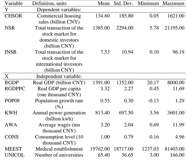
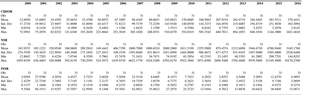
The appendix table 2 below is a summary of the main variables and control variables in this paper. It can be seen that the observed number of all variables is 527, and there is no drawback of missing variables. For the three major variables, the standard deviation of INSR is relatively small, and it can be inferred that its dispersion degree is relatively small compared with the other two variables. For the control variables, the trend concentration is RGDPPC, POP08, AWA and CONS. However, since the data set in this paper covers the data of 31 provinces in 17 years, and the economic development level and economic growth rate of each province also vary greatly, the variables may be processed by first-order difference in subsequent empirical studies to eliminate the trend.
Figure 2. Summary statistics of main variables and control variables, 2000-2016 NT=31x17=527 observations.
Variable Definition, units Mean Std. Dev. Minimum Maximum Y Dependent variables:
CHSOR Commercial housing sales (billion CNY)
134.60 185.80 0.05 1621.00 NSR Total transaction of the
stock market for domestic investors
(billion CNY)
1385.00 2294.00 5.78 21195.00
INSR Total transaction of the stock market for international investors
(billion CNY)
7.53 10.94 0.10 96.19
X Independent variable:
RGDP Real GDP (billion CNY) 1391.00 1352.00 20.17 8000.00 RGDPPC Real GDP per capita
(one thousand CNY)
3.32 2.27 0.45 11.69
POP08 Population growth rate (%)
0.55 0.30 -0.13 1.29
KWH Annual power generation (billion kwh)
813.40 697.50 3.56 3601.00 AWA Average wages (ten
thousand CNY)
3.20 2.04 0.69 11.99
CONS Consumption level (10 thousand CNY)
1.00 0.79 0.16 4.96
MEEST Medical establishment 19762.00 18717.00 1237.03 81403.00 UNICOL Number of universities 65.40 36.65 3.00 166.00
PARK Number of parks 291.20 438.70 1.00 3986.00 RFET Foreign exchange
earnings from tourism (billion CNY)
11.01 17.67 0.01 127.60
RTIE Total import and export (billion CNY)
606.40 1158.00 1.29 6686.00
Note: CNY is Chinese currency Yuan Renminbi, $1=7.10 CNY on May 15, 2020.
5. Methodology
In order to verify the relationship between the real estate market and the stock market in different provinces of China, the empirical model established in this paper takes the annual sales of commercial houses as the dependent variable and the annual transaction of different stock markets as the independent variable. Firstly, the long-term relationship between them will be found by autoregressive distributed lag (ARDL) model. Secondly, the causality between them is explored by error correction model (ECM).
According to Kim and Korhonen (2005), many previous studies have used pooled ordinary least squares (OLS) models to analyse data from multiple countries over a period of time, but this classical method has unavoidable drawbacks, such as the inability of this method to consider non-stationary data. However, based on the dynamic heterogeneous panels proposed by Pesaran and Smith (1995), the dynamic characteristics of the model will no longer be ignored. For the real estate market and the stock market, there are clearly dynamic characteristics. Therefore, the ARDL model is more suitable than the traditional OLS estimation method in this case. Pesaran, Shin and Smith (2001) also mentioned the bound testing approaches of ARDL model in their subsequent studies, which has a greater tolerance for the stationarity of variables.
More specifically, the autoregressive distributed lag (ADRL) form proposed by Pesaran and Smith (1995) is as follows:
𝑦𝑖𝑡 = 𝛼1𝑖+ 𝛼2𝑖𝑡 + 𝛽1𝑖𝑦𝑖,𝑡−1+. . . +𝛽𝑝𝑖𝑦𝑖,𝑡−𝑝+ 𝛾1𝑖𝑥𝑖𝑡 + 𝛾2𝑖𝑥𝑖,𝑡−1+. . . +𝛾𝑞𝑖𝑥𝑖,𝑡−𝑞+ 𝜀𝑖𝑡 i = 1, 2, …, N; t = 1, 2, …, T (1) In the above equation (1), Y is the dependent variable (CHSOR), which represents the commercial housing sales. It can be explained by its own lag value, so the model is
autoregressive. X as the explanatory variables (NSR and INSR), which are related to 2 different stock markets for domestic investors and international investors. They also appear in the form of continuous lag as the other independent variable. T represents the difference in time, N represents the different provinces, εit represents the random error term.
Furthermore, Pesaran et al. (2001) mentioned ARDL bounds testing approach of cointegration in a subsequent study. According to Ozturk and Acaravci (2010), this approach has three advantages: Firstly, this model can be analysed using a formula with regressors of different orders, such as integrated of orders 0 and 1 I(0) and I(1); secondly, the classic Johansen cointegration method is highly reliable only when the number of samples is large, but the ARDL bounds testing approach can accurately handle the cointegration relationship of small samples. Finally, the ARDL method can be used for the cointegration test without even testing the unit root of the variable in advance. However, in the following regression analysis in this article, the unit root test is performed to make the results more reliable. The "optimized" ADRL bound testing approach of Pesaran et al. (2001) is as follows:
∆𝑦𝑖𝑡 = 𝛽0+ ∑ 𝛽𝑖 𝑘 𝑖=1 ∆𝑦𝑖𝑡−𝑖+ ∑ ∆𝑥1𝑖𝑡−𝑗 𝑙 𝑗=0 + 𝛿1𝑦𝑖𝑡−1+ 𝛿2𝑥𝑖𝑡−1+ 𝜀𝑖𝑡 i = 1, 2, …, N; t = 1, 2, …, T; j = 1, 2, …, N (2) Similarly, εit and Δ describe the random error term and the first difference of variables, respectively. Ozturk and Acaravci (2010) suggest following Akaike Information Criterion (AIC) or Schwarz Information Criterion (SBC) for the selection of the optimal lag length. However, Pesaran et al. (2001) also provided the essential hypothesis of this model, that is, the error terms must be independent and identically distributed (iid). This hypothesis will also affect the choice of the optimal lag length. In equation (2), the null hypothesis is H0: δ1 = δ2 = 0. To test this hypothesis, we need to observe the value of the F-test. When the regression result can reject the null hypothesis, it means that the coefficient of the lagging term is not equal to 0, and there is a long-term relationship between the two variables.
Since the ARDL model has an autoregressive structure, the model needs to be dynamic and relatively stable. This means that the inverse roots of the feature equation associated with the model are strictly within the unit circle. When this prerequisite is met, bounds testing can be performed. According to Pesaran et al. (2001), only when bound testing provides a cointegration conclusion can the long-term equilibrium relationship between variables be predicted. Similarly, although the ARDL model can determine the long-term relationship between variables, it also has its own defect, that is, it cannot determine the causal relationship between variables; nor can it describe the direction of this causal relationship. Therefore, this thesis needs to use the dynamic VEC model to explore the causal relationship between independent variables and dependent variables. This paper will use the dynamic VEC model from the research of Ozturk and Acaravci (2010), specified in the following form:
∆𝑦𝑖𝑡 = 𝛼1+ ∑𝑘𝑖=1𝛽𝑖∆𝑦𝑖𝑡−𝑖+∑𝑙𝑗=1𝛽𝑗∆𝑥𝑖𝑡−𝑗+ 𝛾1𝑣𝑖𝑡−1+ 𝑒1𝑖𝑡 (3) ∆𝑥𝑖𝑡 = 𝛼2+ ∑𝑘𝑖=1𝛿𝑖∆𝑦𝑖𝑡−𝑖+ ∑𝑙𝑗=1𝜃𝑗∆𝑥𝑖𝑡−𝑗+ 𝛾2𝑣𝑖𝑡−1+ 𝑒2𝑖𝑡 (4) It is assumed that the error terms in the above equation (3) and (4) have mean 0 and constant variance. The null hypothesis is that xit is not the Granger causing of yit, and yit is not the granger causing of xit. If the null hypothesis is rejected, yit and xit are Granger reasons for each other. Ozturk et al. (2010) proposed three methods to detect Granger causality: first, weak granger causality can be obtained by checking whether the value of βj is equal to 0; second, the velocity of long-term equilibrium dissipation can be obtained by observing the coefficient of the error correction term vit-1; third, strong Granger causality can be determined by H0: βj = βi = 0 or H0: θj = δi = 0. It is worth noting that the coefficient of the error correction term vit-1 reflects the rate at which the variable can eliminate the long-term equilibrium bias. To summarise, the dynamic VEC model captures the strong and weak Granger causality and is an effective complement to the ARDL bounds testing method.
6. Estimation Procedure
6.1 Descriptive statisticsTable 2 in the Appendix demonstrates the descriptive statistics of three key variables in this paper. The mean of commercial building sales (CHSOR) continued to rise in the research range of this paper, from 12.695 in 2000 to 379.442 in 2016. During this period, the average value of real estate sales (CHSOR) decreased in 2008, and the rest years maintained the growth trend. The drop in sales in 2008 was largely due to the global financial crisis. The standard deviation of CHSOR also increases with the change of years. Therefore, this phenomenon is considered to indicate that there are great differences in real estate prices in different provinces and that the real estate development is unbalanced during this period.
For the two aggregated stock markets, the market for domestic investors (NSR) has been more volatile over the past 17 years. The mean has a minimum value of 150.052 and a maximum value of 6786.946. As can be seen from the standard deviation, this value was relatively small before 2006. Since 2007, the standard deviation has increased by 5 times, and this paper can infer that the stock market has been polarized from 2006 to 2007. However, the standard deviation reached its maximum in 2015. It is worth noting that 2015 was the year of the sudden boom in China's stock market, but the sharp increase in standard deviation reflects that the boom was "non-equilibrium" for different provinces. Moreover, the aggregate stock market (INSR) for foreign investors is relatively small. In this research period, the fluctuation is relatively stable, and the dispersion degree does not change much. However, it also experienced a sudden increase in trading volume and standard deviation in 2007 and 2015, which is completely consistent with NSR. But overall, the development of this market in different provinces is relatively stable and equilibrium.
6.2 Correlation test
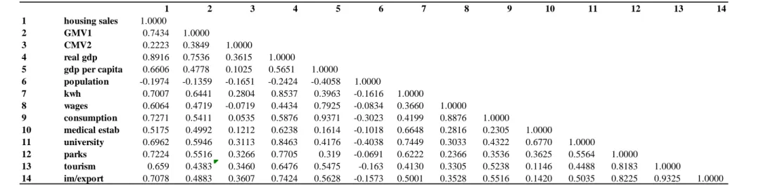
The appendix table 3 illustrates the Pearson correlation coefficient matrix of all variables in this paper. It can be seen that there is no high correlation between the three main variables, so there is no multicollinearity problem. However, for the control variables, real GDP and real estate sales are highly correlated. Therefore, RGDP will not be
considered as the main control variable when the dependent variable is CHSOR. Similarly, there is a high correlation between GDP per capita and household consumption level, which is 0.9371. At the same time, the province's import and export level and tourism foreign exchange income also has a significant correlation. These findings will help us better conduct follow-up robustness tests. For instance, when this paper uses the total import and export volume as the control variable for the robustness test, the tourism board is not taken into account. This is helpful to overcome the errors caused by multicollinearity in regression.
6.3 Panel autoregressive distributed lag (ARDL) estimation method
When conducting panel ARDL model estimation, firstly we need to carry out three steps, namely model definition, descriptive statistics and correlation test. As mentioned earlier in this paper, we should go straight to unit root test and selection of optimal lag length. And then, the cointegration test is considered, which helps us to observe the long-term relationship between the main variables. The second is the Hausman test, which can help us to choose the best analysis method among mean group (MG), pooled mean group (PMG) and dynamic fixed effects (DFE). Finally, we need to estimate the model and organize the causality test.
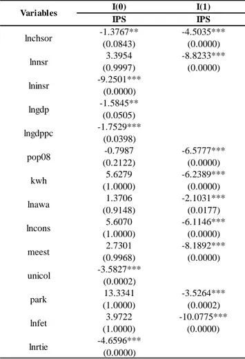
One of the most benefits of panel ARDL method is that it can contain both integrated I(0) and I(1) variables, but it must not have I(2) in the regression. In order to overcome the potential multicollinearity and the high degree of autocorrelation between variables, all the variables related to currency or money in this paper are natural logarithms. In addition, this paper uses the Im, Pesaran and Shin (IPS) method for unit root testing, which assumes that the variable has heterogeneous slopes, which is more in line with the actual situation of the data. Meanwhile, the time trend of variables will not be included in the unit root inspection process. The unit root test results are shown in Table 3 below. All variables are stationary under the condition of I(0) or I(1). For logarithm of GDP (LnGDP), it is not significant at the significance level of 0.05 but significant at the significance level of 0.10, and its I(1) is very "nonstationary". Therefore, LnGDP is included in the I(0) stable group in this paper. The panel unit root test results for all the groups is presented in the Table 3 below.
Table 3. Panel unit root test result for all the groups
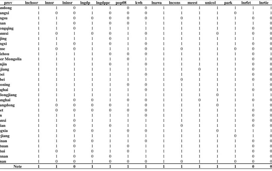
Furthermore, this paper carried out the selection of optimal lags. Few previous academic researches on panel ARDL included control variables. Therefore, this paper learned the previous methods to determine the optimal lag length of the main variables first, and then introduced control variables to determine the optimal lag term conditional on the control variables. We can compare whether the optimal lag length of the main variables changes before and after adding the control variables. Meanwhile, in order not to lose too many degrees of freedom, we set maximum lag length to 1. After that, we should select the most common lag across indicates the provinces. For the variables in this paper, the optimal lag of LnGDP, LnRFET and LnTIE is 0; for other variables, the optimal lag length is 1. The Table 4 in the Appendix shows the summary of the optimal lag of all the variables for different provinces.
The next step is the cointegration test proposed by Pedroni (2004). In fact, there are three kinds of Pedroni cointegration test in the academic field, including time fixed effect, individual fixed effect and both cases. This paper first explores the cointegration
lnchsor lnnsr lninsr lngdp lngdppc pop08 kwh lnawa lncons meest unicol park lnfet lnrtie -6.1146*** (0.0000) -8.1892*** (0.0000) -3.5264*** (0.0002) -10.0775*** (0.0000) 3.9722 (1.0000) -4.6596*** (0.0000) -4.5035*** (0.0000) -6.5777*** (0.0000) -8.8233*** (0.0000) -6.2389*** (0.0000) -2.1031*** (0.0177) 5.6279 (1.0000) 1.3706 (0.9148) 5.6070 (1.0000) 2.7301 (0.9968) -3.5827*** (0.0002) 13.3341 (1.0000) -1.3767** (0.0843) 3.3954 (0.9997) -9.2501*** (0.0000) -1.5845** (0.0505) -1.7529*** (0.0398) -0.7987 (0.2122) I(0) IPS I(1) IPS Variables
relationship among the three main variables. Table 5 in the appendix shows that at the significance level of 0.1, the null hypothesis can be rejected. Note that the alternative assumption is that "all" panels are cointegrated. Therefore, LnCHSOR, LnNSR and LnINSR have cointegration relations. The following cointegration test will gradually include different control variables, because the Pedroni cointegration test can only contain 7 regressors at the same time, while this paper contains 14 control variables. It turns out that for the absolute value of ρ, the groups are greater than panels. This indicates that the null hypothesis can be rejected at the significance level of 0.01, so after adding different control variables, the variables are still cointegrated.
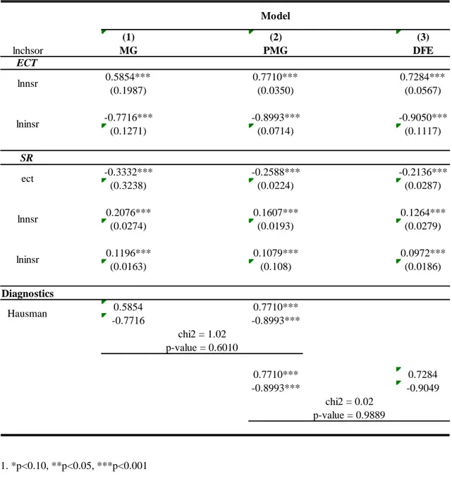
Similarly, we also need to choose the most efficient method between mean group (MG), pooled mean group (PMG) and dynamic fixed effect model (DFE). Therefore, we should use different methods for regression and use Hausman test for filtering. In determining the optimal estimation method, this paper uses only the three most important variables for regression. Because a large number of control variables will lead to so many iterations, which will lead to the generation of PMG results and ultimately affect the results of Hausman test. Table 6 shows that p-value is equal to 0.6010, which is greater than 0.05. This indicates that the null hypothesis cannot be rejected at the significance level of 0.05. Therefore, the model supports the PMG estimator.
Furthermore, the Hausman test is carried out on the relatively efficient PMG model and DFE in this thesis. We are only interested in the result of Hausman test, which is shown in appendix table 6. Between the PMG and DFE estimator, if the p-value is greater than 0.05, we cannot reject the null hypothesis. The p-value equals to 0.9989, which indicates that PMG is more efficient than DFE for the main variables in this paper.
When using PMG to estimate model, only a broad result can be obtained in the long-run relationship due to the homogeneity assumption of PMG. However, for the short-term relationship between variables, the differences before different provinces can be observed in this paper. In fact, when we used MG for estimation of the model, we could observe differences in the long-term relationship between variables in 31 different provinces due to the absence of homogeneity assumption. However, because of the Hausman test results do not support the use of MG model, this paper takes MG method as a supplement to the conclusion, rather than as the focus of the study. In the process of PMG estimation, the
results cannot be obtained when the control variables are greater than three. When the fourth control variables are included in the regression, even after 74 iterations, no valid results can be obtained. Therefore, the 11 control variables in this paper were added to 5 groups of PMG estimates. Appendix table 5 shows the results of PMG. Firstly, when the control variables only include LnGDP and LnGDPPC, LnNSR has no significant impact on LnCHSOR, which means that the growth rate of domestic stock market turnover has no direct impact on the growth rate of real estate market turnover. However, in the short term, LnNSR in most provinces had no significant effect on LnCHSOR at the significance level of 0.1, and only three provinces had significant relationship. For LnINSR, only 7 provinces had the correlation between LnINSR and LnCHSOR, and the regression results of most provinces were still insignificant at the significance level of 0.1.
Furthermore, new control variables POP08 and KWH are replaced in the next regression. In the long run, LnINSR still has a significant positive effect on LnCHSOR, while LnNSR still has an insignificant effect on LnCHSOR. However, in the short-term regression results of individual provinces, we can find that LnNSR has a significant effect on LnCHSOR in some provinces. In this case, LnNSR in 12 provinces had positive or negative effects on LnCHSOR in the short term. Similarly, LnINSR in 14 provinces also significantly affected LnCHSOR. The new control variable changed the significance of the coefficient of LnNSR and LnINSR in some provinces. However, there is no universal or absolute result. In addition, when LnAWA and LnCONS were used as control variables, the significance between LnCHSOR, LnNSR and LnINSR did not change over the long term. But in the short term, only three provinces had significant LnNSR effects on LnCHSOR. The difference is that when we change the control variables to MEEST and UNICOL, the p-value of LnNSR is 0.008, and the hypothesis of no correlation type can be rejected. In this case, when the LnNSR increases by 1, the LnCHSOR will increase by 0.1365. However, in this case, the effect of LnINSR on LnCHSOR is not significant, so we cannot reject the null hypothesis that the two are unrelated.
Finally, when we introduced PARK, LnRFET and LnRTIE, the p-value of all variables was less than the significance level of 0.05. In the long term, for every 1 increase in LnINSR, the LnCHSOR decreases by 0.3875, and there is a negative correlation between the those two. All the other variables were in the same direction as LnCHSOR. In the
short term, the main variables of each province still show different correlations. Among them, the major variables of province Shanghai, Guangdong, Fujian and Ningxia showed a strong correlation, and both LnNSR and LnINSR were significantly correlated with LnCHSOR. This means there is a correlation between real estate and equities in the four provinces. For other provinces, however, the regression results were insufficient to capture the strong correlation between the two variables.
The final step is the causality test. This causality relationship can also be determined by using the significance of the ECT, long-run coefficients and short-run coefficients, which captures the be causality. Since the data in this paper are panel data and contain multiple provinces and times, the traditional VEC model cannot be used. First, this paper recalls the PMG approach to causality test data as a whole, and does not include the control variable, which has shown in the Table 6 in the Appendix. By examining the coefficient of PMG regression results, we found that LnNSR and LnINSR had significant long-term causal relationship with LnCHSOR. When LnNSR and LnINSR were used as dependent variables, the other two variables still had a long-term causal relationship and were significant at the significance level of 0.05. This means that there is a significant causal relationship between LnNSR, LnINSR and LnCHSOR in the long term. In other words, there is a long-term causal relationship between the real estate market and the two stock markets. Interestingly, for the short-run, there was also a significant short-term causality between the three major variables. It is worth noting that the short-term PMG regression can provide an error correction term that reflects the joint result. It can be seen that when LnCHSOR is taken as the dependent variable, the two independent variables related to stocks tend to be balanced at a speed of 0.2588. When the LnNSR is taken as the dependent variable, the rate becomes 0.9013. When LnINSR is taken as the dependent variable, the equilibrium rate will be 1.5863.
In addition, when we used the PMG full method to regression the three main variables, we could capture the causality between variables in a single province. The appendix table 7 shows that the two independent variables of provinces Jiangsu, Chongqing, Guangdong, Fujian, Ningxia, and Zhejiang have a short-term causality with the dependent variables. For LnNSR and LnCHSOR, only province Henan and province Qinghai had a short-term causality, and LnINSR and LnCHSOR had a short-term causality in all other provinces.
This means that the relationship between real estate and equities varies from province to province. The correlation and causality between real estate and stock are not universal even in the same country.
5.4 Discussion of the estimation result
For the dataset in this essay, probably the estimation is not as accurate as in the previous literature. Most of the previous studies were based on international data to find representative stock market indicators and real estate indicators for analysis. For the purposes of this paper, China mainland's provinces are unlikely to have their own independent stock markets. Therefore, this paper divides the stock market into two parts, and carries on the weighted treatment. This has the advantage of weakening the homogeneity of the aggregate stock market. But in the long run, the causality between the stock market and the real estate market can only be accurately observed at the national level. And the short-term cause-and-effect relationship between them can be captured at the provincial level. This study uses the inter-provincial differences in information which is lost when using aggregate national level data.
The previous assumption in this paper was that in China mainland, the real estate market and the stock market have a two-way causality relationship. As alternative investment products, they will divide up the currency in investors' hands. However, empirical analysis shows that this is not the case. For example, in very few provinces, the short-term causality between Chinese housing and housing stocks goes both ways. On the other hand, the stock market for foreign investors may have a greater impact on the real estate market in the short term than the stock market for domestic investors. The reason for this phenomenon may be that China's foreign direct investment (FDI) continued to increase from 2000 to 2016 in the research range of this paper. Mainland China has also attracted outside investors. For the investment of domestic investors, the increase in the total investment of foreign investors will be relatively significant.
It is important to note that different provinces have different main industries, reflecting possible different causal relationships. The finding also overturns assumptions. At the beginning of this paper, it is predicted that the correlation and causality between housing and stocks will be regionalized. For example, the eastern region is relatively developed in economy, so the housing and stocks market is relatively active, and they will show a
two-way causality relationship. The middle and western provinces show a single causal relationship in different directions. But in fact, the regression results show that the causal relationship between housing and stock markets does not have much influence on the economic region where the province is located. On the contrary, the province's main industry or the pillar of the economy may indirectly determine the cause and effect. In other word, real estate and the two aggregate stock markets have mutual influence and cause and effect on each other in the long run. However, the short-term relationship between them will be affected by other factors, some of which were identified here and considered as control variables.
7. Conclusion and Recommendations
7.1 Summary and recommendationsIn conclusion, all the regression and analysis in this paper confirm that there is a correlation and causality between the real estate market and the stock market, both in the long term and the short term. However, this causal relationship varies from one province to another province, and there is no uniform conclusion to generalize all provinces. The relationship between stocks and real estate is estimated using different estimation methods and testing procedures. It can be found by Hausman test that pooled mean group (PMG) is most suitable for analysing and processing the data in this paper. The estimation result show that in the 31 different provinces of China, there is a long-term cause-and-effect relationship between the property market and the two combined stock markets (domestic and foreign investors) that has a significant effect on each other. But in the short term, the causal relationship between the real estate market and the stock market is inconsistent.
As mentioned earlier, this paper divides the different provinces of China into three different economic regions, namely the eastern area, middle area and western area. For provinces Jiangsu, Chongqing, Guangdong, Fujian, Ningxia and Zhejiang, both stock markets have a significant causal relationship with the real estate market. Four of them are from eastern provinces and two are from western provinces. In addition, there was only a significant causal relationship between the stock market and the real estate market of domestic investors in two provinces, all of which came from the central provinces. The