Mobile Device Gaze Estimation with Deep Learning: Using Siamese Neural Networks

Mobile Device Gaze

Estimation with Deep

Learning

Using Siamese Neural Networks

JULIEN ADLER

KTH ROYAL INSTITUTE OF TECHNOLOGY

Estimation with Deep

Learning

Using Siamese Neural Networks

JULIEN ADLER

Master in Computer Science Date: November 25, 2019

Supervisor: György Dàn, Ryo Kurazume Examiner: Robert Lagerström

School of Electrical Engineering and Computer Science

Swedish title: Ögonblicksuppskattning för mobila enheter med djupinlärning

Abstract

Gaze tracking has already shown to be a popular technology for desktop de-vices. When it comes to gaze tracking for mobile devices, however, there is still a lot of progress to be made. There’s still no high accuracy gaze track-ing available that works in an unconstrained setttrack-ing for mobile devices. This work makes contributions in the area of appearance-based unconstrained gaze estimation. Artificial neural networks are trained on GazeCapture, a publicly available dataset for mobile gaze estimation containing over 2 million face im-ages and corresponding gaze labels. In this work, Siamese neural networks are trained to learn linear distances between face images for different gaze points. Then, during inference, calibration points are used to estimate gaze points. This approach is shown to be an effective way of utilizing calibration points in order to improve the result of gaze estimation.

Sammanfattning

Ögonblickspårning har redan etablerat sig som en populär teknologi för sta-tionära enheter. När det dock gäller mobila enheter så finns det framsteg att göra. Det saknas fortfarande en lösning för ögonblickspårning som fungerar i en undantagsfri miljö för mobila enheter. Detta examensarbete ämnar att bi-dra till en sådan lösning. Artificiella neurala nätverk tränas på GazeCapture, en allmänt tillgänglig datasamling som består av över 2 miljoner ansiktsbilder samt korresponderande etikett för ögonblickspunkt. I detta examensarbete trä-nas Siamesiska neurala nätverk för att lära sig det linjära avståndet mellan två ögonblickspunkter. Sedan utnyttjas en samling med kalibreringsbilder för att estimera ögonblickspunkter. Denna teknik visar sig vara ett effektivt sätt att nyttja kalibreringsbilder med målet att förbättra resultatet för ögonblicksesti-mering.

1 Introduction 1

1.1 Research Questions . . . 3

1.2 Scope . . . 3

1.3 Outline . . . 3

2 Background 4 2.1 Appearance-Based Unconstrained Gaze Estimation . . . 4

2.1.1 Problem Description . . . 4

2.1.2 Accuracy Metrics . . . 5

2.1.3 The GazeCapture Dataset . . . 5

2.2 Artificial Neural Networks . . . 6

2.2.1 Artificial Neuron . . . 6

2.2.2 Neural Networks and Connected Layers . . . 7

2.2.3 Learning and Backpropagation . . . 8

2.2.4 Convolutional Layers . . . 9

2.2.5 Depthwise Separable Convolutions . . . 11

2.2.6 Pooling Layers . . . 13

2.3 Transfer Learning . . . 13

2.4 Similarity Learning . . . 14

2.4.1 Siamese Neural Network . . . 14

2.5 Calibration . . . 15

3 Related Work 17 3.1 Eye Tracking for Everyone . . . 17

3.1.1 iTracker: a Deep Neural Network for Eye Tracking . . 17

3.1.2 Calibration with SVR . . . 18

3.2 MobileNets . . . 19

3.3 A Differential Approach for Gaze Estimation with Calibration 21 3.4 It’s Written All Over Your Face . . . 22

4 Siamese Regression for GazeCapture 24

4.1 The Siamese Neural Network for Regression . . . 24

4.1.1 Neural Network Architecture . . . 25

4.1.2 Training the Siamese Neural Network . . . 26

4.1.3 Gaze Inference Using the Siamese Neural Network . . 28

4.2 Intermediate Experiments . . . 29

5 Results 31 5.1 Siamese Neural Network and Calibration Points for Gaze Es-timation . . . 31

5.1.1 Inference Time . . . 32

5.2 Miniature Models . . . 33

6 Discussion 35 6.1 Mobile Phones vs Tablets . . . 35

6.2 Effect of Increasing Calibration Points . . . 35

6.3 Even Spread or Random . . . 36

6.4 The Efficacy of Siamese Neural Networks for Gaze Estimation with Calibration . . . 36

6.5 Inference Time . . . 37

6.6 Transfer Learning from ImageNet to GazeCapture . . . 37

6.7 Fine-tuning for Specific Device and Orientation . . . 37

6.8 Increased Data Quantity for Gaze Difference . . . 38

6.9 iTracker vs MobileNet . . . 38

6.10 Depthwise Separable Convolutions . . . 38

7 Conclusions 39 7.1 Transfer Learning . . . 39

7.2 Calibration Points with Siamese Neural Networks . . . 39

7.3 Future Work . . . 40

Introduction

Recent advances in gaze estimation technology have given rise to a variety of eye tracking applications[1]. Gaze tracking has already seen use in the auto-motive industry1, retail and advertisement[2], health care[3, 4, 5] and medical testing[6] and the market for eye tracking is expected to keep growing in com-ing years[7].

A widely available, non-intrusive solution for gaze tracking on portable devices could facilitate the lives of people with motor disabilities [8], under-standing user behaviour[9] or improving user experience in tasks such as read-ing[10].

Gaze estimation has been and continues to be an active field of research, containing various unsolved challenges. Gaze estimation techniques are often categorized as either model-based or appearance-based[11]. Current commer-cial eye tracking relies on specific hardware components[12] and/or a combi-nation of algorithms[13] using corneal reflections, calibration points and ge-ometrical 3D modeling of the eye. This falls in the category of model-based gaze estimation[11]. While the model-based approach works well, it often relies on certain constraints in order to work effectively. These constraints may include limitation of head movement, specific hardware components or demands related to the background environment. Such methods which are sometimes referred to as constraint-based gaze estimation[14] cannot work in all scenarios.

In contrast to model-based methods, appearance-based gaze estimation techniques attempt to map gaze location directly from eye or face images[11]. It’s believed that these appearance-based methods could be useful for uncon-strained gaze estimation[15]. In this context, "unconuncon-strained" refers to the lack

1

https://tobii.com/tech/products/automotive/

of prior assumptions regarding user appearance, environment, camera, head pose etc.

There are many factors that make eye tracking on off-the-shelf mobile de-vices more challenging than classical eye tracking[16]. Firstly, mobile dede-vices have limited computational power compared to stationary devices. Further, in the natural use case of mobile devices, it’s impractical for users to adhere to the same constraints required in the case of stationary devices. The unconstrained setting makes for a lack of reliability in terms of the environment, illumination conditions, distance and angle from eye to camera as well as camera quality which makes eye tracking for mobile devices more challenging than for PCs or head-mounted devices.

Recently, several attempts have been made to tackle the problem of un-constrained gaze estimation with deep learning[17, 18]. Following the well-known successes of neural networks and deep learning for various computer vision tasks[19, 20], the hope is that deep learning will be able to solve this challenging problem as well.

This work aims to explore the usage of deep learning for unconstrained appearance-based gaze estimation in mobile devices. In particular, this work will explore neural networks utilizing depthwise separable convolutions which have already proven their efficiency in other computer vision tasks[21, 22]. depthwise separable convolutions can reduce the number of parameters (and required memory) compared to standard convolutions while maintaining learn-ability; a highly desirable quality for mobile devices which have limited mem-ory. Furthermore, this work analyzes the usefulness of transfer learning for gaze estimation: a technique that has been commonly used for computer vi-sion tasks. Transfer learning aims to extract useful features across different domains in order to reduce the training time or improve the final accuracy for the target domain[23, 24]. Finally, this work is concerned with calibration points and how they may be used in the case of deep learning for unconstrained gaze estimation. Calibration points are already a vital component in the com-mercial model-based eye trackers. Calibration allows models to make use of information regarding the differing appearance or pose for specific users as well as how the light is reflected depending on the environment. In the case of appearance-based models for unconstrained gaze estimation with mobile de-vices, an attempt to incorporate calibration points involved feeding the features from the last fully connected layer to a SVM (Support Vector Machine)[12]. In this work, the utilization of Siamese neural networks as a way to incorporate calibration points is examined.

1.1

Research Questions

The objective of this work is to make meaningful empirical scientific exper-iments that will contribute to furthering the field of appearance-based gaze capture. This work aims to give an answer about the following questions:

• How beneficial is cross-domain transfer learning in the task of mobile

device gaze estimation?

• How should calibration points be incorporated in order to improve the

gaze estimation accuracy?

1.2

Scope

The final goal is to improve learning-based inference models for unconstrained gaze estimation while taking into consideration the memory constraints of a mobile device. While this inference model should ultimately be deployable on a mobile device, this work is not concerned with optimizing for real-time eye tracking nor developing an application that makes use of eye tracking.

1.3

Outline

Chapter 2 describes the relevant background theory and chapter 3 presents some state-of-the-art solutions that serve as inspiration for this thesis.

Chapter 4 defines the specific experiments and implementation details. This includes analyzing and preparing datasets, developing and training models as well as testing the models for gaze point inference. Chapter 5 contains the results from all the experiments and these findings will be analyzed in chapter 6. Finally, chapter 7 draws conclusions related to the research questions that were posed in chapter 1.

Background

This chapter presents the fundamental theoretical concepts related to the work done. In the first section, appearance-based unconstrained gaze estimation is defined and the GazeCapture dataset is introduced. In subsequent sections, neural networks and their relevant components are explained. In the final sec-tions, Siamese neural networks are described and it is mentioned how they may be used in combination with calibration points.

2.1

Appearance-Based Unconstrained Gaze

Estimation

An appearance-based model takes some image frame(s) of the subject as input and produces gaze direction as output. The task of gaze estimation is described as "unconstrained" when no specific demands are placed on the input image. This means that the inference model should be capable of estimating the gaze for any user, in any natural setting. In particular, there are no requirements such as head pose, distance, angle etc. The goal is to make an eye tracker that works reliably on any mobile phone, using no special equipment apart from the front camera.

2.1.1

Problem Description

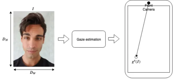
The gaze estimation task may be formulated as gaze point regression where the goal is to minimize euclidean distance between the predicted gaze point and the true gaze point. The input is a normalized face input image I ∈ [0, 1]DW,DH,DC

, taken with a mobile device front camera, where DW is the im-age width, DH is the image height and DC is the number of color channels. In

our case, I is a RGB image where the dimensions are given as (DW, DH, DC) =

(224, 224, 3). Given I, the goal is to predict a gaze point gp(I) ∈ R2 _{on the} plane of the mobile device screen, where gp(I) is the coordinate distance in centimeters from the device front camera.

Figure 2.1: Gaze estimation for mobile devices

2.1.2

Accuracy Metrics

While all appearance-based models have some image frame(s) as input and gaze direction as output, there is no standard way to represent gaze direction and accuracy[1]. The common accuracy metrics are angular error (in degrees), absolute distance (pixels, mm), relative distance (percentage). A survey was performed, using 200 different research articles on gaze based algorithms and applications (see Table 1), showing angular error is more popular in general but absolute error is more popular for mobile devices.

2.1.3

The GazeCapture Dataset

There are many publicly available datasets for the task of gaze estimation. GazeCapture is one such dataset containing almost 2,500,000 datapoints from 1450 different people[12]. This dataset was gathered on various iOS mobile devices in an unconstrained setting. The datapoints include the image frame taken by the front camera, valid face and eye crops as well as the correspond-ing gaze point labels. These labels are given as the x and y distance from the camera in centimeters. It needs to be taken into consideration though that, as in the real world, not all of these frames contain valid face frames (no face,

Table 2.1: Popularity of various accuracy metrics [25] Eye Tracking Platform No. of Sur-veyed Papers No. using Metric: De-gree No. using Metric: Per-centage No. using Metric: Oth-ers (pixels, mm) Desktop 69 44 16 9 Handheld 21 3 9 9 Automotive 35 11 14 10 Head-mounted 57 37 2 18

closed eyes etc.) After filtering for valid frames containing a detected face and opened eyes this dataset contains 1,490,959 datapoints.

2.2

Artificial Neural Networks

Supervised learning algorithms build statistical models from data in order to perform certain tasks. A popular learning algorithm is the artificial neural net-work. Gaining in popularity as computational power keeps increasing, neural networks are a powerful tool for solving various problems. As the name sug-gests, neural networks are inspired by the structure of a brain.

2.2.1

Artificial Neuron

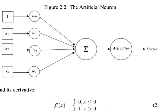
An artificial neural network is composed of a collection of connected nodes called artificial neurons. Each one of these artificial neurons take some inputs x1, x2, ..., xn as well as a bias input. The neuron has a set of trainable

pa-rameters (weights) w0, w1, ..., wn. When the neuron is fed inputs it produces an output depending on an activation function which takes the sum of all the weighted inputs. With the bias always being 1, the output can be formulated as Output = Activation( n X i=0 wi∗ xi) . (2.1) The activation function is some nonlinear, differentiable function. Most commonly used today is the ReLU (Rectified Linear Unit). It is defined as

f (x) =

(

0, x ≤ 0

Figure 2.2: The Artificial Neuron

and its derivative:

f0(x) =

(

0, x ≤ 0

1, x > 0 . (2.3) There are various different activation functions to choose from but studies show that ReLU reliably produces good results.

2.2.2

Neural Networks and Connected Layers

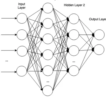
As mentioned, a complete neural network can be constructed by connecting a multitude of artificial neurons. Rather than adding them individually, neurons are typically aggregated in layers. The first layer is often referred to as the input layer. The final layer is called the output layer, and the intermediate layers are called hidden layers. Input is fed to the input layer which transforms and propagates the information forward through the rest of the neural network. The output is the final activation produced by the output layer.

A layer Li is considered fully connected when every one of its inputs are

connected to every output of the previous layer Li−1. The fully connected

neural network is the simplest type of neural network, consisting purely of fully connected layers of artificial neurons. Figure 2.3 illustrates such a fully connected neural network, with 2 hidden layers and 2 neurons in the output layer.

Since the number of parameters in fully connected layers grows quickly with the number of neurons, such naive neural networks are not commonly used for complex tasks such as image recognition. Fortunately, there are other layers that can reduce the number of parameters for a neural network. Such

Figure 2.3: A Fully Connected Neural Network With 2 Hidden Layers

layers include pooling layers and convolutional layers which will be described in a later subsection.

2.2.3

Learning and Backpropagation

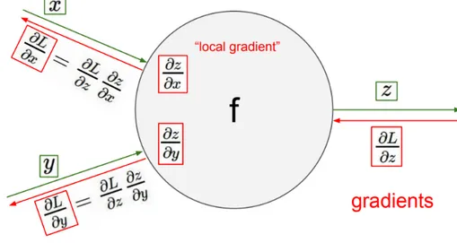
The previous sections described how inputs are forward propagated through the neural network, transforming inputs to outputs. The neural network also needs to be able to learn from data in order to produce useful outputs. This is done by adjusting the weights in such a way that the produced output will match the data. The weights are adjusted using backpropagation. Backprop-agation is a gradient-based optimization algorithm which exploits the chain rule to efficiently adjust the weights layer by layer. After feeding the neural network labeled data, e.g. some input image vector x and its corresponding label l, and producing an output y, we use some loss function L(y, l) = E between the neural network output and data label. Then, by using the chain rule the gradient can be calculated layer by layer. For some neuron with output o and weights wi, the gradient is

∂E ∂wi = ∂E ∂o ∂o ∂wi . _(2.4)

functions are differentiable in order to calculate the local gradients and update all the weights in the neural network during training.

Figure 2.4: A single neuron with two inputs x and y, activation function f. The backpropagation step is shown in red.

2.2.4

Convolutional Layers

Convolutional layers are a vital component in neural networks concerned with learning tasks related to images. Neural networks that utilize convolutional layers are often referred to as CNNs (Convolutional Neural Networks). We know that pixels in an image are most useful in the context of neighbouring pixels, so the idea is to save parameters by looking at smaller parts of the image instead of all the pixels at once (in contrast to fully connected layers). Convolutional layers are a set of filters. One can think of these filters as 2d matrices. The convolution operation is to "slide" these filters across a feature map, performing element-wise multiplications at each position. The feature map can be the input image or any intermediate output at any layer in the neural network. The sum of the multiplications are the outputs for the new image, as illustrated in Figure 2.5 and 2.6. The convolution is a differentiable operation and therefore these filters are trainable parameters.

Since images typically have a color channel for red, green and blue channel values as well as the spatial width and height, the initial input feature map and feature maps produced at any point in the neural network are usually 3d rather than 2d. The filters need to match the number of dimensions. Each convolution layer has some number of these trainable filters, producing a new channel for

Figure 2.5: A 4x4 greyscale image and a 3x3 filter

Figure 2.6: The output given the image and filter in Figure 2.5

each filter. For example, applying 6 (5 × 5 × 3) filters on a (32 × 32 × 3) image produces a (28 × 28 × 6) image as seen in Figure 2.7.

A standard convolutional layer takes a feature map F of dimensions DF ×

DF × M as input and produces a feature map G of dimensions DG× DG× N

as output, where DF is the spatial width and height of a square input feature

map, M is the number of input channels, DG is the spatial width and height

of a square output map, N is the number of output channels. Using a standard convolution kernel K of size DK × DK × M × N , where DK is the spatial dimension of the kernel, the output feature map is computed as:

Gk,l,n=

X

i,j,m

Ki,j,m,n∗ Fk+i−1,l+j−1,m (2.5)

multi-Figure 2.7: A convolution layer with 6 filters produces 6 output channels

plicatively on the number of input channels M , output channels N , kernel size DK × DK and the feature map size DF × DF. I.e., the convolutional operation has a computational cost of:

DK∗ DK ∗ M ∗ N ∗ DF ∗ DF . (2.6)

Figure 2.8: Standard convolution filters[22]

2.2.5

Depthwise Separable Convolutions

Utilized in the popular MobileNets[22] and Inception[21] model architectures, depthwise separable convolutions have been effective in a wide range of use-cases such as object detection, finegrain classification, face attributes and large-scale geo-localization. The idea behind depthwise separable convolution is to speed up the calculations by factorizing the standard convolution into a depth-wise convolution followed by a 1 × 1 (also called a point-depth-wise) convolution.

The depthwise convolution applies a single filter to each input channel. The pointwise convolution is then applied to combine the outputs of the depthwise convolution. The combination of a depthwise convolution followed by a point-wise convolution is similar to a factorization of the standard convolution in the sense that they produce an output feature map of the same dimensions. The depthwise convolution can be formulated as:

ˆ Gk,l,m = X i,j ˆ Ki,j,m∗ Fk+i−1,l+j−1,m (2.7)

where ˆK is the depthwise convolutional kernel of size DK× DK× M , using

one filter per input channel where the mthfilter is applied to the mthchannel in

F to produce the mth channel of ˆG. Since the depthwise convolution doesn’t

combine input channels to create new features, it only has the computation cost of:

DK∗ DK ∗ M ∗ DF ∗ DF . (2.8)

Figure 2.9: Depthwise convolution filters[22]

Figure 2.10: Pointwise convolution filters[22]

Next, the 1 × 1 pointwise convolution is applied to the output feature map of the depthwise convolution. This combination of depthwise convolution and pointwise convolution is what’s called a depthwise separable convolution. In total, the computational cost is:

This means that the total computational complexity is reduced compared to the standard convolution. In fact, it is a reduction by a factor of N. In the case of MobileNet which uses 3×3 convolutions, the depthwise separable convolution takes between 8 to 9 times less computation than standard convolutions with only a small reduction in accuracy[22].

2.2.6

Pooling Layers

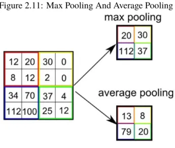
Pooling layers are used to reduce the size of feature maps. Pooling layers are a way to reduce the computational requirements by extracting dominant features. The most common types of pooling are max pooling and average pooling. Similarly to convolutional layers, the pooling operation looks at small patches of an image at a time. As the names suggest, max pooling returns the maximum value and average pooling returns the average value from each kernel.

Figure 2.11: Max Pooling And Average Pooling

2.3

Transfer Learning

An interesting observation is that the scale of a machine learning model and the amount of required data to learn a task has an almost linear relationship[26]. The expressive space of a model must be large enough to discover the patterns in the data. Conversely, a model could be considered underutilized when data is insufficient. Transfer learning has proven to be an efficient technique in domains where it’s difficult to collect a large dataset[27]. It has been shown

in many cases that pre-training on a Source Domain can effectively "trans-fer" lower level features and ultimately improve the prediction accuracy in a different Target Domain.

2.4

Similarity Learning

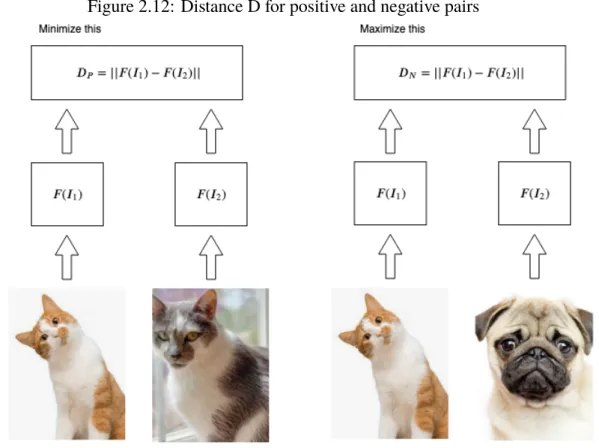
Instead of directly learning a classification or regression problem, similarity learning aims to learn how similar or related two objects are. For images, this typically involves extracting some features from two images, then using a similarity function to get a similarity measurement between the features of the two different images. Let I1, I2be the two images and F (I1), F (I2) be the

extracted features. Then, the standard similarity learning goal is to optimize for a metric of similarity between the extracted features. To achieve this, we can define a distance between the features using the euclidean norm:

D = ||F (I1) − F (I2)|| = ||F (I1) − F (I2)||2. (2.10)

2.4.1

Siamese Neural Network

Siamese neural networks are practical for similarity learning, because they can jointly optimize the feature representation of the images conditioned on the similarity function being used. In other words, similarity learning con-veniently happens in an end-to-end manner. Siamese neural networks have been used successfully in a variety of computer vision tasks in areas such as object tracking and identity verification. The Siamese neural network gets it name from the use of two identical neural networks; two neural networks with shared weights take two different images and then combines the output. In practice however, this is usually implemented using a single neural network with two different input channels so as to save on memory.

In order for the CNN to learn properly, the loss function must make a dis-tinction between positive (similar) and negative (dissimilar) pairs of images. Commonly used for classification is the contrastive loss. It can be defined as: L(Y, I1, I2) = (1 − Y )LP(D) + Y LN(D) , (2.11) LP(I1, I2) = 1 2(D) 2_, (2.12) LN(I1, I2) = 1 2{max(0, m − D)} 2_, (2.13)

Figure 2.12: Distance D for positive and negative pairs

where Y is a binary label to indicate a positive or negative pair. Y = 0 for positive pairs and Y = 1 for negative pairs. In other words, LP becomes the

loss for positive pairs and LN the loss for negative pairs. I1, I2, D are defined

in the previous section 2.4. This is just one possible way to train a Siamese neural network for classification and there are variations in the regression case as well, which will be further explored in the next chapters.

2.5

Calibration

When it comes to unconstrained gaze estimation there are user-specific vari-abilities that an inference model may benefit from learning. These include gaze range, illumination conditions, and personal differences. According to experiments by [15] these account for 25%, 35% and 40% performance gap respectively. This is true for model-based approaches as well, and so com-mercial 3D geometrical shape-based eye tracking systems utilize calibration points to account for these variabilities. When it comes to appearance-based

Figure 2.13: A standard Siamese CNN

models, one attempt to use calibration points involved feeding the features from the last fully connected layer to a SVM (support vector machine) for subject-specific gaze adaptation[12]. Another appearance-based solution in-volved training a Siamese neural network to learn about the similarity between eye images, then during inference estimated gaze points with a random set of reference gaze images[28].

Related Work

This chapter aims to give an overview of previous works. This chapter only in-cludes works that are particularly related to and served as inspiration or build-ing blocks for this thesis project. If the reader is interested, more details about their respective implementations may be found in the original papers.

3.1

Eye Tracking for Everyone

Krafka et al. describes a neural network architecture for eye tracking[12] which achieved state of the art results for the GazeCapture dataset. The next section introduces their architecture and results which will be used as a base-line for the experiments of this thesis.

3.1.1

iTracker: a Deep Neural Network for Eye

Track-ing

The proposed solution, the iTracker, is a multi channeled input neural network trained on the GazeCapture dataset in order to learn unconstrained gaze esti-mation: mapping an input frame taken by a mobile device front camera to the corresponding gaze coordinates on the screen. As illustrated in Figure 3.1, the neural network has 4 input channels. The first and second inputs, the right and left eye crops, go through a series of convolutional layers. Notably, the con-volutional layers, denoted CONV-E1, CONV-E2, CONV-E3 and CONV-E4, have shared weights for both eye crops. Their output feature vectors are com-bined through concatenation and fed to a fully connected layer FC-E1. The third input, a face crop, goes through a series of convolutional layers, denoted CONV-F1, CONV-F2, CONV-F3 and CONV-F4, followed by two fully

Figure 3.1: The iTracker architecture

nected layers FC-F1 and FC-F2. The fourth input is a binary mask indicating the position of the previously mentioned face crop image relative to the orig-inal input frame. This binary mask goes through two fully connected layers FC-FG1 and FC-FG2. Finally, the features from FC-E1, FC-F2 and FC-FG2 are combined with a fully connected layer FC1, and the last fully connected layer FC2 produces the gaze prediction output.

The frames are split into image crops of the persons face, right eye, left eye and a face grid which is a binary mask used to indicate the location of the face crop within the original frame.

The iTracker attained state-of-the-art results[12], as summarized in table 3.1. The error is reported in cm; lower is better. Aug. refers to dataset aug-mentation and tr and te indicates train and test set, respectively. The results are taken separately for mobile phones and tablets. Further, a dot error value is reported, which is the average error of all the datapoints corresponding to the same gaze coordinates within the dataset. The iTracker* refers to a model which was fine-tuned to each device and orientation. The authors note that this was particularly helpful for tablet devices, likely because of the large pro-portion of phones (85%) in the dataset compared to tablets (15%).

3.1.2

Calibration with SVR

The results are improved further by applying SVR (support vector regression) to features extracted by the iTracker, specifically from the FC1 layer from Fig-ure 3.1. The SVR model was trained with a varying amount of calibration

Table 3.1: The results of iTracker without calibration images.

The Aug. column signifies whether data augmentation was done or not. Fur-ther, iTracker* was fine-tuned for specific device and orientation.

Model Aug. Mobile phone

error dot error

Tablet

error dot error iTracker None 2.04 1.62 3.32 2.82

iTracker te 1.84 1.58 3.21 2.90

iTracker tr 1.86 1.57 2.81 2.47

iTracker tr + te 1.77 1.53 2.83 2.53 iTracker* tr + te 1.71 1.53 2.53 2.38

points and the various results are summarized in table 3.2.

Table 3.2: The results of iTracker using SVR for calibration points. iTracker* was fine-tuned for specific device and orientation

Model Calibration points

Mobile phone error dot error

Tablet

error dot error

iTracker 0 1.77 1.53 2.83 2.53 iTracker 4 1.92 1.71 4.41 4.11 iTracker 5 1.76 1.50 3.50 3.13 iTracker 9 1.64 1.33 3.04 2.59 iTracker 13 1.56 1.26 2.81 2.38 iTracker* 0 1.71 1.53 2.53 2.3 iTracker* 4 1.65 1.42 3.12 2.96 iTracker* 5 1.52 1.22 2.56 2.30 iTracker* 9 1.41 1.10 2.29 1.87 iTracker* 13 1.34 1.04 2.12 1.69

Using 13 calibration points for the SVR, the model which was fine-tuned for device and orientation achieved the best results.

3.2

MobileNets

The MobileNets are a class efficient of neural network models introduced by AG. Howard et al[22]. They are based on depthwise separable convolutions which were described in section 2.2.5. These neural networks are all built with a similar structure: a single standard convolutional layer followed by a

series of depthwise separable convolutions. That is, an alternating series of depthwise convolutions followed by 1 × 1 (pointwise) convolutions. An ex-ample of a full MobileNet architecture can be seen in table 3.5. The idea is to replace all the standard convolutions, which are comparatively computation-ally expensive, with depthwise separable convolutions. Figure 3.2 illustrates a standard 3x3 convolutional layer, on the left, and the depthwise convolutional layer that replaces it, on the right.

Figure 3.2: Left: standard convolutional layer. Right: depthwise separable convolutional layer. [22]

The MobileNet architecture has managed achieve an accuracy comparable to state-of-the-art results on classification tasks such as ImageNet, while dras-tically reducing the number of parameters. Table 3.3 compares MobileNet and a standard convolutional version of itself. We can see a trade-off of accuracy and computation/memory in terms of number of parameters and Mult-Adds. A notable reduction of computation and required parameters results in a rela-tively small loss of accuracy, demonstrating the efficiency of depthwise sepa-rable convolutions. While the standard convolutional version does effectively achieve a 1.56% higher accuracy, it also utilizes 597.62% more parameters. Table 3.4 shows how the depthwise separable version of MobileNet compares to other popular, larger, models.

Table 3.3: Depthwise separable vs fully convolutional MobileNet Model ImageNet Accuracy Million MultAdds Million Parameters Conv MobileNet 71.7% 4866 29.3 MobileNet 70.6% 569 4.2

Table 3.4: MobileNet compared to other popular models Model ImageNet Accuracy Million MultAdds Million Parameters MobileNet 70.6% 569 4.2 GoogleNet 69.8% 1550 6.8 VGG 16 71.5% 15300 138

3.3

A Differential Approach for Gaze

Estima-tion with CalibraEstima-tion

In a work within the area of gaze estimation for computer screens, G. Liu et al. proposed a Siamese neural network structure as a way to utilize calibration points[28]. This work is done on a dataset called MPIIGaze, which consists of images labeled with an angle of gaze in relation to the camera. However, instead of learning the direct gaze angle, the Siamese neural network learns the angular difference between two different eye images; it is referred to as the differential approach. During training the neural network was given two input eye images through different image channels. Their output feature maps were flattened and concatenated into a combined feature vector. Lastly, the features went through an intermediate fully connected layer before the output layer. The architecture is illustrated in Figure 3.3.

Table 3.5: The MobileNet Architecture. Conv refers to a standard convolution layer followed by batch normalization and ReLU activation. Conv dw is a depthwise convolution followed by batch normalization and ReLU activation.

Type / Stride Filter shape Input size Conv / s2 3 × 3 × 3 × 32 224 × 224 × 3 Conv dw / s1 3 × 3 × 32 dw 112 × 112 × 32 Conv / s1 1 × 1 × 32 × 64 112 × 112 × 32 Conv dw / s2 3 × 3 × 64 dw 112 × 112 × 64 Conv / s1 1 × 1 × 64 × 128 56 × 56 × 64 Conv dw / s1 3 × 3 × 128 dw 56 × 56 × 128 Conv / s1 1 × 1 × 128 × 128 56 × 56 × 128 Conv dw / s2 3 × 3 × 128 dw 56 × 56 × 128 Conv / s1 1 × 1 × 128 × 256 28 × 28 × 128 Conv dw / s1 3 × 3 × 256 dw 28 × 28 × 256 Conv / s1 1 × 1 × 256 × 256 28 × 28 × 256 Conv dw / s2 3 × 3 × 256 dw 28 × 28 × 256 Conv / s1 1 × 1 × 256 × 512 14 × 14 × 256 Conv dw / s1 3 × 3 × 512 dw 14 × 14 × 512 Conv / s1 1 × 1 × 512 × 512 14 × 14 × 512 Conv dw / s1 3 × 3 × 512 dw 14 × 14 × 512 Conv / s1 1 × 1 × 512 × 512 14 × 14 × 512 Conv dw / s1 3 × 3 × 512 dw 14 × 14 × 512 Conv / s1 1 × 1 × 512 × 512 14 × 14 × 512 Conv dw / s1 3 × 3 × 512 dw 14 × 14 × 512 Conv / s1 1 × 1 × 512 × 512 14 × 14 × 512 Conv dw / s1 3 × 3 × 512 dw 14 × 14 × 512 Conv / s1 1 × 1 × 512 × 512 14 × 14 × 512 Conv dw / s2 3 × 3 × 512 dw 14 × 14 × 512 Conv / s1 1 × 1 × 512 × 1024 7 × 7 × 512 Conv dw / s2 3 × 3 × 1024 dw 7 × 7 × 1024 Conv / s1 1 × 1 × 1024 × 1024 7 × 7 × 1024 Avg Pool / s1 Pool 7 × 7 7 × 7 × 1024 FC / s1 1024 × 1000 1 × 1 × 1024 Softmax / s1 Classifier 1 × 1 × 1000

3.4

It’s Written All Over Your Face

X. Zhang et al. who released the MPIIGaze dataset have also proposed various different deep learning models. Early state-of-the-art results were achieved

by using a combination of eye crops and head rotation angle as input to the model[30]. More recently, X. Zhang et al. proposed a deep learning model taking full face crops as input rather than eye crops. This approach improved upon the previous results, indicating that information from the full face region can be of benefit[31].

Siamese Regression for

Gaze-Capture

This chapter describes the proposed Siamese neural network for gaze differ-ence regression. The architecture of the Siamese neural network is explained in detail. Next, a description is given about how the neural network was trained and tested; this includes dataset processing and training parameters as well as how calibration points were utilized to infer gaze points from gaze difference predictions during testing. Furthermore, some intermediate experiments are included: these were made in the development process of the final proposed architecture.

4.1

The Siamese Neural Network for

Regres-sion

Similar to the Siamese neural network used for classification (section 3.2.2), the input consists of two images I1, I2. In the regression case, however, there are no positive or negative samples so there’s no need for a contrastive loss function. Instead, all the input pairs are of the same subject and the goal of the Siamese neural network is to predict a linear distance dp(I1, I2) ∈ R2between

the two gaze points on the screen. In other words, the goal is to learn the prediction dp(I1, I2) corresponding to the ground truth gaze difference:

dgt(I1, I2) = ggt(I1) − ggt(I2), (4.1)

where ggt(I1), ggt(I2) ∈ R2are the labeled ground truth gaze points for I1, I2.

An illustration is provided in Figure 4.1, where the predicted gaze difference dp(I1, I2) (in red) can be represented visually as a vector from I2to I1.

Figure 4.1: The gaze difference task

4.1.1

Neural Network Architecture

In this work, the Siamese neural network takes cropped face images as inputs I1, I2. These are fed into a Siamese version of MobileNet without the last two

layers, that is the Softmax/s1 classifier and the FC/s1 layer, have been removed (refer to table 3.5 for details). The 7×7×1024 features are flattened and the flattened 50176 features F (I1), F (I2) are fed into a layer

D = F (I1) − F (I2) (4.2)

followed by a final linear activation layer.

Note that the layer D is the simple difference rather than the absolute dif-ference between the features. It is utilizing the asymmetrical nature of two datapoints for this learning problem. That is, it should be expected that the gaze difference for two images when switching place in the input is the same gaze difference but opposite direction:

dgt(I1, I2) = −dgt(I2, I1) . (4.3)

Therefore, defining D as in equation 4.2 maintains the overall symmetry, be-cause

D(I1, I2) = −D(I2, I1), (4.4)

dp(I1, I2) = −dp(I2, I1) (4.5)

also holds; and so the neural network learns the same weight update, regardless of which input position it gets fed two data points.

Figure 4.2: The Siamese neural network for regression

4.1.2

Training the Siamese Neural Network

Dataset

The model was trained using a subset of the GazeCapture dataset, taking the 1,490,959 data points containing valid face and eye recognitions from 1471 different subjects. The subset was further split into subsets for training, vali-dation and testing. These subsets contain respectively 1,251,983, 59,480 and 179,496 datapoints. The face crops had an image resolution of 224×224. The dataset has some over-represented points, namely the 13 calibration points for each device type in the dataset. Figure 4.3 shows a plot of the distribution of gaze points in the dataset, where the two axes represent spatial distance from the device camera in centimeters. Since both the training set and the test set had similarly uneven distributions, this was not considered as a problem and thus ignored. Further, the dataset contains some data points where the de-tected face had negative coordinates. This could mean that the dede-tected face square starts outside of the original frame, resulting in a smaller face crop. All these data points in the training set with negative face coordinates were skipped when training the neural network.

Figure 4.3: Distribution of gaze points in the dataset.

Weight Update And Loss Function

The Siamese neural network was trained using the MAE (Mean Absolute Er-ror) loss function:

L = 1 N X (I1,I2)∈SC ||dp_(I 1, I2) − dgt(I1, I2)|| , (4.6)

where N is the batch size, SC is a subset of the dataset containing the same subject C. Because of computation costs, instead of training with all |SC|2 combinations, each datapoint is chosen just once as I1with a random I2every

epoch.

The weights were updated using the Adam method for 5 epochs, then with classic stochastic gradient descent for 1 more epoch using a learning rate of 0.001 and batch size of 16.

4.1.3

Gaze Inference Using the Siamese Neural

Net-work

Gaze Points From Gaze Difference

The neural network output is just a linear difference, but the gaze estimation task is about predicting an actual gaze point. In order to get an actual gaze point from an input image I, at least one calibration data point R is required; the actual gaze point prediction gp(I) can then be taken as the calibration point plus the linear difference:

gp(I) = ggt(R) + dp(I, R) . _(4.7)

Furthermore, multiple calibration points may be used; the gaze point predic-tion then becomes the mean:

gp(I) = 1 |SC_|

X

R∈SC

ggt(R) + dp(I, R) , _(4.8)

where SC is the set of calibration images.

Random Versus Evenly Spread Calibration Gaze Points

During testing, the set of calibration images SCwere chosen in different ways. Experiments included varying the amount of calibration images |SC|, trying 1, 5, 9 and 13 number of calibration points. The first way to pick calibration points was by random selection. The second way was to pick evenly spread calibration points across the screen.

Improving Inference Time

For mobile devices, reducing computation time is vital. Using the Siamese neural network with |SC| calibration points, the computation time for inference on a single image I is:

T = (1 + |SC|)(M + K) , _(4.9) where M is the computation time for a single pass of I through the first part of the neural network to produce a feature vector F (I) and K is the compu-tation time of a pass through the rest of the neural network to produce a gaze difference prediction given two feature vectors, i.e. dp(F (I), F (R)). Since M > K, the model was split into two parts; one for computing the features

Figure 4.4: Evenly spread calibration points: Illustration of how they were chosen for in the case of 1 (grey), 5 (red), 9 (green) and 13 (blue) points.

from images, the other for computing the gaze difference prediction. Then, by pre-computing and keeping a collection of the feature vectors for all the cali-bration images, the total computation time for an input image can be reduced to:

T = (1 + |SC|)K + M . _(4.10) .

4.2

Intermediate Experiments

When it comes to neural network architectures, there are an infinite number of ways to design them. Furthermore, there are various weight-updating al-gorithms and training parameters, such as learning rate, often referred to as

hyper-parameters. Therefore, multiple models are often trained in deep learn-ing projects in order to achieve the best results and to test different ideas. However, it is time consuming and computationally expensive to train deep neural networks on full resolution images using large datasets. Therefore, the following intermediate experiments were performed on a smaller subset of the data using lower resolution images. These intermediate experiments were not expected to achieve great results compared to the state-of-the-art solution. Nonetheless, they are included here in the hope that comparing their results with each other may provide scientific value.

Emulating iTracker

A smaller version of the iTracker model was implemented. It was trained using a subset of GazeCapture, containing 100,000 data points for training, 10,000 data points for validation and 10,000 data points for testing; all with images of 128×128 resolution and containing valid face/eye detections. It should be noted that the motivation behind this experiment is to emulate the efficiency of the iTracker architecture, not to achieve a model with highest possible ac-curacy; this has already been done in the original work and the various results of iTracker may be found in section 3.1.

A Siamese Version of iTracker

Similar to the previously described the Siamese neural network for regression, a Siamese version of iTracker was also constructed and trained with the same 128×128 resolution subset containing 100,000 data points for training, 10,000 data points for validation and 10,000 data points for testing. Thus, this network takes 4×2 inputs and predicts a linear distance between the two samples’ gaze points. It should be noted that this Siamese iTracker, like the other Siamese neural networks, need to use at least one calibration image during inference to produce a gaze estimation from the neural network output.

Pre-Trained MobileNet for GazeCapture

Two different experiments were performed with MobileNet. Two versions of MobileNet was trained with the same 128×128 resolution subset containing 100,000 data points for training, 10,000 data points for validation and 10,000 data points for testing. First, a regular version of MobileNet was trained and tested. Second, a version that had been pre-trained on the ImageNet dataset was fine-tuned. Both models took cropped face images as input.

Results

This chapter shows the gaze error for the above-mentioned models. For the final Siamese neural network model, it is shown how varying the number of calibration images affects the results. Further, it is tested in practice whether the inference time can be reduced by splitting the model as described in section 4.2.3.

5.1

Siamese Neural Network and Calibration

Points for Gaze Estimation

This section presents the results of the Siamese neural network, described in section 4.1. It was tested using random calibration points (Table 5.1) and evenly spread calibration points (Table 5.2). It is shown in Table 5.1 and 5.2 how choosing 1, 5, 9 and 13 calibration points affects the gaze estimation re-sults in both cases. The result was taken for all the phones and tablets in the test set separately, so as to be comparable with the previous results of the iTracker. In Table 5.3, the results of the Siamese neural network is compared with the results of iTracker+SVR when utilizing 13 calibration points. Note that while no fine-tuning was done for device and orientation in the case of the Siamese network, the results of the fine-tuned iTracker (denoted iTracker*) is still in-cluded as a baseline. Thus, the error value presented in Table 5.3 represents the best result of iTracker, that is the state-of-the-art result for GazeCapture when utilizing 13 calibration points. If the reader is interested in the full re-sults of iTracker, including the dot error, it can be found in Table 3.1 and 3.2.

Table 5.1: Siamese neural network with random calibration set Number of Cal

Points

Mobile phone error Tablet error

1 2.14 3.25

5 1.59 2.45

9 1.50 2.35

13 1.48 2.30

Table 5.2: Siamese neural network with evenly spread calibration set Number of Cal

Points

Mobile phone error Tablet error

1 1.69 2.26

5 1.45 2.25

9 1.38 2.05

13 1.33 1.97

Table 5.3: Siamese neural network compared with iTracker+SVR, both us-ing 13 evenly spread calibration points. The model fine-tuned for device and orientation is denoted as iTracker*.

Model Mobile phone error Tablet error

iTracker+SVR 1.56 2.81

iTracker*+SVR 1.34 2.12 Siamese neural

net-work

1.33 1.97

5.1.1

Inference Time

This is a evaluation of the optimization method described in section 4.1.3. By splitting the model and keeping a collection of calibration features, the infer-ence time can be reduced. Table 5.4 shows the average time when performing inference, computing on a Quadro K620 GPU with 2GB memory. The split-ting model optimization method is compared to the naive way of re-compusplit-ting features for all the 13 calibration points.

Table 5.4: Measurement in seconds Method Inference Time

Seconds Naive version 0.3368 Saving features 0.0672

5.2

Miniature Models

In the intermediate experiments, described in section 4.2, miniature versions of iTracker and MobileNet were compared using a smaller subset of data, con-sisting of 128×128 resolution face images. Further, a pre-trained version of MobileNet was imported and fine-tuned for the gaze estimation problem. This version had been pre-trained on ImageNet and was fine-tuned for GazeCap-ture. These miniature models were all trained using early stopping with a patience of 5 epochs. The weights were updated using the Adam method. A batch size of 16 was used and the initial learning rate was set to 0.001. The final epoch number can be seen in Table 5.5. Note that no calibration images are necessary for the regular iTracker and MobileNet. In these experiments, the results of phones and tablets were taken together.

Table 5.5: Miniature iTracker and MobileNet

Model error epochs

iTracker 4.32 9

MobileNet 3.97 24

Pre-Trained MobileNet

3.94 21

Further, Siamese versions of the iTracker and MobileNet were tested. These miniature Siamese models were also trained with a batch size of 16, early stop-ping with a patience of 5 epochs and using the Adam method with a learning rate of 0.001. They were trained using the same smaller subset of data using 128×128 resolution images. Note that these models require at least one cal-ibration image to produce a gaze estimation from the neural network output. In this case, 13 random calibration points were chosen during testing.

Table 5.6: Siamese iTracker and MobileNet with 13 calibration points

Model error epochs

iTracker 4.20 16

Discussion

This chapter highlights some notable results and possible implications from the experimental results.

6.1

Mobile Phones vs Tablets

It may be observed that inference on mobile phones has a lower error than on tablets. This is true for Table 5.1, 5.2 and 5.3, as well as the previous work pre-sented in 3.1 and 3.2. One explanation is that this is due to the imbalance in the dataset, containing about 85% phones and 15% tablets. The error discrepency still exists after fine-tuning for specific device type, as seen in 3.1 and 3.2. Another explanation is that the problem naturally gets inherently harder when increasing the problem space in the form of an increased interval of possible gaze points.

6.2

Effect of Increasing Calibration Points

Looking at Table 5.1 and 5.2, a clear trend can be observed related to the num-ber of calibration points. Increasing the numnum-ber of calibration points results in a lower error for gaze estimation in all of the Siamese neural network ex-periments. It seems to be a non-linear relationship however, and diminishing returns can be seen when increasing the number of calibration points. Al-though the method of utilizing calibration points is different, the same can be seen in Table 3.1 and 3.2 in the previous results of iTracker.

6.3

Even Spread or Random

When looking at table 5.1 and 5.2, it can be seen that choosing calibration points in a systematic manner gives better results. Rather than choosing ran-dom calibration points, using evenly spread calibration points reduce the error for all the gaze estimation tests, using 1, 5, 9 or 13 calibration points. The biggest error difference is observed when comparing the cases with a single calibration point; a random calibration point gives an error of 2.14 (phones) and 3.25 (tablets) while using a single calibration point in the center of the device screen gives an error of 1.69 (phones) and 2.26 (tablets). The error difference between the two approaches still exists when using 13 calibration points but does get smaller, 1.48 vs 1.33 and 2.30 vs 1.97, when increasing the number of calibration points.

6.4

The Efficacy of Siamese Neural Networks

for Gaze Estimation with Calibration

The results of the Siamese neural network compares well to the current state-of-the-art iTracker, even outperforming it under fair conditions. As described in section 3.1, the iTracker implemented things like data enhancement, device-specific fine-tuning and the dot error method, neither of which were imple-mented in this project. While the dot error method is an important improve-ment, it requires multiple input images corresponding to the same gaze point. As this project only deals with single input image inference, the results can only be compared to the error value, not the dot error value.

It can be seen from table 5.3 that, in the case of single input image and 13 calibration points and no device-specific fine-tuning, this Siamese net outper-forms the iTracker+SVR for calibration approach. The iTracker+SVR achieved an error of 1.56 (phones) and 2.81 (tablets). After fine-tuning for specific de-vice and orientation, iTracker*+SVR achieved an error of 1.34 (phones) and 2.12 (tablets).

Even without fine-tuning for device and orientation, the Siamese neural network achieves an error of 1.33 (phones) and 1.97 (tablets); outperforming the iTracker+SVR approach for both phones and tablets.

6.5

Inference Time

Table 5.4 shows that saving a collection of pre-computed features of the cali-bration images rather than re-computing them every time may yield a speed-up during inference. The implementation of this method on the machine using a Quadro K620 GPU with 2GB memory resulted in an average 501% speed-up. This shows that the main computation cost during forward propagation is from computing the image features. This makes sense since this part of the neural network is a lot bigger than the regression layer; it contains most of the neurons.

6.6

Transfer Learning from ImageNet to

Gaze-Capture

Table 5.5 shows the result of two miniature versions of MobileNet (with 128x128 image input); one was pre-trained on ImageNet and the other was trained from scratch on the GazeCapture subset. While the pre-trained version did finish training earlier, epoch 21 instead of 24, the difference in error is small. This experiment shows no drastic improvement. However, it cannot be concluded that cross-domain transfer learning could be useful for gaze estimation. It is possible that the ImageNet dataset does not include images that are relevant enough to produce useful features in the gaze estimation task. Therefore, fur-ther investigations using ofur-ther datasets should still be made. It would be in-teresting to see whether pre-training on datasets containing more human faces would be more beneficial.

6.7

Fine-tuning for Specific Device and

Ori-entation

While no final fine-tuning was done in this project, section 3.1 mentions how the iTracker was fine-tuned for specific device and orientation, yielding a clear improvement of the results. It can be seen in Table 5.3 how the iTracker* dras-tically reduces the error for both mobile phones and tablets. It can reasonably be expected that fine-tuning may further reduce the error for the Siamese neu-ral network as well.

6.8

Increased Data Quantity for Gaze

Differ-ence

In reformulating the gaze point estimation task as a gaze difference task, an inherent property arises: increased number of data samples. Since any com-bination of two data samples in the dataset make up one data sample in the gaze difference task, there’s a possible quadratic increase of available data samples by using every possible combination. That is, if the dataset contains N samples originally, the new dataset for gaze difference contains N ∗(N −1) unique samples. However, to test the data quality, that is whether all these new samples are beneficial, for a large dataset like GazeCapture is difficult to test because of the sheer time it would take to train a network using every possible combination of data samples.

6.9

iTracker vs MobileNet

Table 5.5 also shows a version of iTracker, trained on the same, smaller, dataset. In this case the error was higher than that of MobileNet.

Further, Table 5.6 shows Siamese versions of these miniature models. It seems from the result that turning the iTracker into a Siamese only improves the results slightly. On the other hand, the Siamese MobileNet version achieves quite a low error value of 2.21, considering the smaller size images (128x128) and amount of data points (100,000).

6.10

Depthwise Separable Convolutions

As mentioned in section 2.2.5, the pre-study shows that neural networks uti-lizing depthwise separable convolutions may train faster than traditional con-volutional neural networks. Whether depthwise separable convolutions result in an accuracy increase depends on computation time and resources. Looking at the results in Table 5.5 and 5.6, it shows that the MobileNet model (us-ing depthwise separable convolutions) achieve better results than the iTracker model (using standard convolutions) on the miniature dataset. However, there are too many architectural differences between these two networks to draw any conclusions about the efficacy of depthwise separable convolutions. While the final model in this project also utilizes depthwise separable convolutions and achieved good accuracy, it cannot either be directly attributed to the use of depthwise separable convolutions.

Conclusions

In this chapter, concise answers are given to the research questions stated in section 1.1. Conclusions are drawn from the points raised in the discussion chapter. Finally, some suggestions are given regarding future work related to the topic of this thesis.

7.1

Transfer Learning

The first research question posed was regarding the benefit of cross-domain transfer learning. As mentioned in section 6.6, no considerable improvement was seen in the experiment concerned with cross-domain transfer learning from ImageNet to GazeCapture. Whether transfer learning from ImageNet for gaze estimation is beneficial or not remains unconclusive. However, it is still possible that another dataset may be useful for cross-domain transfer learn-ing for gaze estimation. In order to test this, further investigations uslearn-ing other datasets should be made.

As mentioned in section 6.7, the results of iTracker already clearly show that fine-tuning a model for a specific device yields clear accuracy improve-ments; this is a sort of transfer learning that is useful for the task of gaze esti-mation, however it is not cross-domain.

7.2

Calibration Points with Siamese Neural

Networks

The second research question posed was regarding the use of calibration points and how they may be incorporated to improve gaze estimation accuracy. The

final Siamese model of this project outperforms the previous state-of-the-art model on the GazeCapture dataset, showing that Siamese neural networks are an effective way to make use of calibration points to improve results in the area of unconstrained gaze estimation.

7.3

Future Work

There are a number of interesting directions that remain to be explored. Firstly, it is reasonable to expect further error decrease if the Siamese neural network was fine-tuned for specific device and orientation similarly to the iTracker*. Moving even further in this direction, fine-tuning for specific subjects could also be of particular interest with Siamese neural networks considering that N calibration images become N ∗ (N − 1) unique samples as mentioned in section 6.8.

Additionally, it could be interesting to see whether the error for this model would decrease as drastically as in the case of the iTracker when using the dot error method mentioned in section 3.1.

Further, it could be interesting to see whether another dataset, perhaps con-taining more human faces, would be more beneficial for cross-domain transfer learning.

Finally, it may be worth looking into new ways of incorporating calibration points to increase the accuracy.

[1] Anuradha Kar and Peter M. Corcoran. “A Review and Analysis of Eye-Gaze Estimation Systems, Algorithms and Performance Evaluation Meth-ods in Consumer Platforms”. In: IEEE Access 5 (2017), pp. 16495– 16519.

[2] Tracy Harwood and Martin Jones. “Mobile Eye-Tracking in Retail Re-search”. In: Dec. 2014, pp. 183–199. isbn: 978-3-319-02867-5. doi: 10.1007/978-3-319-02868-2_14.

[3] Jon Patricios et al. “Eye tracking technology in sports-related concus-sion: a systematic review and meta-analysis”. In: Physiological

Mea-surement 39 (Nov. 2018). doi: 10.1088/1361-6579/aaef44.

[4] Uzma Samadani. “A new tool for monitoring brain function: Eye track-ing goes beyond assesstrack-ing attention to measurtrack-ing central nervous sys-tem physiology”. In: Neural Regeneration Research 10 (Aug. 2015), p. 1231. doi: 10.4103/1673-5374.162752.

[5] Deborah L. Levy et al. “Eye tracking dysfunction in schizophrenia: characterization and pathophysiology.” In: Current topics in behavioral

neurosciences 4 (2010), pp. 311–47.

[6] Thomas Koester et al. “The Use of Eye-Tracking in Usability Testing of Medical Devices”. In: Proceedings of the International Symposium on

Human Factors and Ergonomics in Health Care 6.1 (2017), pp. 192–

199. doi: 10 . 1177 / 2327857917061042. eprint: https : / / doi . org / 10 . 1177 / 2327857917061042. url: https : / / doi.org/10.1177/2327857917061042.

[7] https://www.grandviewresearch.com/industry-analysis/ eye-tracking-market. Accessed: 2019-04-25.

[8] Raffaela Amantis et al. “Eye-tracking assistive technology: Is this effec-tive for the developmental age? Evaluation of eye-tracking systems for children and adolescents with cerebral palsy”. In: vol. 29. Sept. 2011, pp. 489–496. isbn: 9781607508137. doi: 10 . 3233 / 978 1 -60750-814-4-489.

[9] Kai Kunze et al. “My Reading Life: Towards Utilizing Eyetracking on Unmodified Tablets and Phones”. In: Proceedings of the 2013 ACM

Conference on Pervasive and Ubiquitous Computing Adjunct Publica-tion. UbiComp ’13 Adjunct. Zurich, Switzerland: ACM, 2013, pp. 283–

286. isbn: 978-1-4503-2215-7. doi: 10.1145/2494091.2494179. url: http : / / doi . acm . org . focus . lib . kth . se / 10 . 1145/2494091.2494179.

[10] Ralf Biedert et al. “Text 2.0”. In: CHI ’10 Extended Abstracts on

Hu-man Factors in Computing Systems. CHI EA ’10. Atlanta, Georgia,

USA: ACM, 2010, pp. 4003–4008. isbn: 978-1-60558-930-5. doi: 10. 1145 / 1753846 . 1754093. url: http : / / doi . acm . org . focus.lib.kth.se/10.1145/1753846.1754093.

[11] D. W. Hansen and Q. Ji. “In the Eye of the Beholder: A Survey of Mod-els for Eyes and Gaze”. In: IEEE Transactions on Pattern Analysis and

Machine Intelligence 32.3 (Mar. 2010), pp. 478–500. issn: 0162-8828.

doi: 10.1109/TPAMI.2009.30.

[12] Kyle Krafka et al. “Eye Tracking for Everyone”. In: IEEE Conference

on Computer Vision and Pattern Recognition (CVPR). 2016.

[13] H. R. Chennamma and Xiaohui Yuan. “A Survey on Eye-Gaze Tracking Techniques”. In: CoRR abs/1312.6410 (2013). arXiv: 1312 . 6410. url: http://arxiv.org/abs/1312.6410.

[14] W. Maio, J. Chen, and Q. Ji. “Constraint-based gaze estimation without active calibration”. In: Face and Gesture 2011. Mar. 2011, pp. 627–631. doi: 10.1109/FG.2011.5771469.

[15] Xucong Zhang et al. “MPIIGaze: Real-World Dataset and Deep Appearance-Based Gaze Estimation”. In: CoRR abs/1711.09017 (2017). arXiv: 1711. 09017. url: http://arxiv.org/abs/1711.09017.

[16] Erroll Wood and Andreas Bulling. “EyeTab: Model-based Gaze Esti-mation on Unmodified Tablet Computers”. In: Proceedings of the

Sym-posium on Eye Tracking Research and Applications. ETRA ’14. Safety

doi: 10.1145/2578153.2578185. url: http://doi.acm. org.focus.lib.kth.se/10.1145/2578153.2578185. [17] Joseph Lemley et al. “Efficient CNN Implementation for Eye-Gaze

Es-timation on Low-Power/Low-Quality Consumer Imaging Systems”. In:

CoRR abs/1806.10890 (2018). arXiv: 1806.10890. url: http://

arxiv.org/abs/1806.10890.

[18] Xucong Zhang et al. “MPIIGaze: Real-World Dataset and Deep Appearance-Based Gaze Estimation”. In: IEEE Transactions on Pattern Analysis

and Machine Intelligence 41 (2019), pp. 162–175.

[19] Md. Zahangir Alom et al. “The History Began from AlexNet: A Com-prehensive Survey on Deep Learning Approaches”. In: (Mar. 2018). [20] Paheding Sidike et al. The History Began from AlexNet: A

Comprehen-sive Survey on Deep Learning Approaches. Nov. 2018.

[21] François Chollet. Xception: Deep Learning with Depthwise Separable

Convolutions. cite arxiv:1610.02357. 2016. url: http://arxiv.

org/abs/1610.02357.

[22] Andrew G. Howard et al. “MobileNets: Efficient Convolutional Neural Networks for Mobile Vision Applications”. In: CoRR abs/1704.04861 (2017). arXiv: 1704.04861. url: http://arxiv.org/abs/ 1704.04861.

[23] Chuanqi Tan et al. “A Survey on Deep Transfer Learning”. In: CoRR abs/1808.01974 (2018). arXiv: 1808.01974. url: http://arxiv. org/abs/1808.01974.

[24] L. Shao, F. Zhu, and X. Li. “Transfer Learning for Visual Categoriza-tion: A Survey”. In: IEEE Transactions on Neural Networks and

Learn-ing Systems 26.5 (May 2015), pp. 1019–1034. issn: 2162-237X. doi:

10.1109/TNNLS.2014.2330900.

[25] Anuradha Kar and Peter Corcoran. “Performance Evaluation Strategies for Eye Gaze Estimation Systems with Quantitative Metrics and Visu-alizations”. In: Sensors 18 (Sept. 2018). doi: 10.3390/s18093151. [26] Chuanqi Tan et al. “A Survey on Deep Transfer Learning: 27th Inter-national Conference on Artificial Neural Networks, Rhodes, Greece, October 4–7, 2018, Proceedings, Part III”. In: Oct. 2018, pp. 270–279. isbn: 978-3-030-01423-0. doi: 10.1007/978- 3- 030- 01424-7_27.

[27] S. J. Pan and Q. Yang. “A Survey on Transfer Learning”. In: IEEE

Transactions on Knowledge and Data Engineering 22.10 (Oct. 2010),

pp. 1345–1359. issn: 1041-4347. doi: 10.1109/TKDE.2009.191. [28] Gang Liu et al. “A Differential Approach for Gaze Estimation with

Cal-ibration”. In: BMVC. 2018.

[29] Gang Liu et al. “A Differential Approach for Gaze Estimation”. In:

CoRR abs/1904.09459 (2019). arXiv: 1904 . 09459. url: http :

//arxiv.org/abs/1904.09459.

[30] Xucong Zhang et al. “Appearance-based Gaze Estimation in the Wild”. In: Proc. of the IEEE Conference on Computer Vision and Pattern

Recog-nition (CVPR). June 2015, pp. 4511–4520.

[31] Xucong Zhang et al. “It’s Written All Over Your Face: Full-Face Appearance-Based Gaze Estimation”. In: 2017 IEEE Conference on Computer

Vi-sion and Pattern Recognition Workshops (CVPRW) (2016), pp. 2299–