http://www.diva-portal.org
This is the published version of a paper presented at ASME Turbo Expo 2019:
Turbomachinery Technical Conference and Exposition, GT 2019, 17 June 2019 through 21
June 2019.
Citation for the original published paper:
Sielemann, M., Thorade, M., Claesson, J., Nguyen, A., Xin, Z. et al. (2019)
Modelica and functional mock-up interface: Open standards for gas turbine simulation
In: Proceedings of the ASME Turbo Expo American Society of Mechanical Engineers
(ASME)
https://doi.org/10.1115/GT2019-91597
N.B. When citing this work, cite the original published paper.
Permanent link to this version:
MODELICA AND FUNCTIONAL MOCK-UP INTERFACE: OPEN STANDARDS FOR
GAS TURBINE SIMULATION
Michael Sielemann, Matthis Thorade Modelon Deutschland GmbH Munich and Hamburg, Germany
Jim Claesson Modelon AB Lund, Sweden
Anh Nguyen Modelon Inc
Glastonbury, Connecticut, USA
Xin Zhao, Smruti Sahoo and Konstantinos Kyprianidis
Mälardalen University Västerås, Sweden ABSTRACT
This paper introduces two physical modeling standards in the gas turbine and cycle analysis context. Modelica is the defacto standard for physical system modeling and simulation. The Functional Mock-Up Interface is a domain-independent standard for model exchange (“engine decks”). The paper summarizes key language concepts and discusses important design patterns in the application of gas turbine simulation concepts to the acausal modeling language. To substantiate how open standards are applicable to gas turbine simulation, the paper closes with two application examples, a conventional unmixed turbofan thermodynamic cycle and weight analysis as well as an electrically boosted geared turbofan.
NOMENCLATURE
DAE Differential algebraic equation FMI Functional Mock-Up Interface FMU Functional Mock-Up Unit GSP Gas Turbine Simulation Program GTF Geared Turbofan
HPC High pressure compressor HPS High pressure shaft HPT High pressure turbine
IPC Intermediate pressure compressor JPL Jet Propulsion Library
LPC Low pressure compressor LPS Low pressure shaft LPT Low pressure turbine NGV Nozzle guide vane
NPSS Numerical Propulsion System Simulation OPR Overall pressure ratio
TET Turbine Entry Temperature
PROOSIS PRopulsion Object Oriented SImulation Software
𝐴𝑒 Cross section area 𝑐𝑝 Specific heat capacity
𝐟 Differential algebraic equation system
𝐠 Initialization equations for differential alg. equation system
𝑘 Turbine mixing pressure loss constant 𝑀 Mach Number 𝑝0 Total pressure 𝑝𝑠 Static pressure 𝑡 Time 𝑇𝑠 Static temperature 𝐱 State variables 𝑣 Flow velocity 𝐰 Algebraic unknowns w Mass flow rate Θ Entropy function
𝜓 Ratio of cooling to inlet gas mass flow rate INTRODUCTION
The last decades saw tremendous efficiency and sustainability improvements of aircraft propulsion using turbofan technology. However, due to intrinsic limitations, it is becoming increasingly difficult to maintain this trend [1]. Proceedings of ASME Turbo Expo 2019: Turbomachinery Technical Conference and Exposition GT2019 June 17-21, 2019, Phoenix, Arizona, USA
Following [2], the overall efficiency of a propulsion system can be considered to be proportional to the product of thermal and propulsive efficiency. To achieve thermal efficiency improvements, the Overall Pressure Ratio (OPR) and the Turbine Entry Temperatures (TET) of the cycles are being increased in an incremental way since the last few decades and are approaching peak values (approximately 1900-2000K TET and around 45-50 cycle OPR). Material limits, turbine cooling, emissions, and losses in the last stage of the high pressure compressor (HPC) may now impose fundamental limits to the thermal efficiency. Improvements in propulsive efficiency are well achievable via reduction in fan pressure ratio and increase in bypass ratio. However, these improvements are deteriorated by losses through lowered transmission efficiency, increased nacelle weight and higher drag due to larger frontal area [3]. In case these limits indeed turn out to be fundamental ones, different and more integrated concepts will be required to yield further efficiency and sustainability improvements.
The range of potential alternatives is large and can hardly be enumerated. We mention two, the supercritical bottoming cycle [4] and hybrid electric propulsion concepts such as the parallel hybrid (e.g., Sugar Volt [5]) or the turbo-electric concept (e.g., STARC-ABL [6], N3-X [7]). In the former, exhaust heat is recovered via a supercritical closed power cycle, in the latter gas turbine thrust and power generation is combined with distributed electrical thrusters, “boost” via energy storage and the like. To understand and design such alternatives, engineers need efficient modeling and simulation, which covers the relevant engineering domains. Such modeling and simulation capability can be implemented by extending domain-specific gas turbine modeling and simulation packages with the new unconventional aspects, or by adopting openly standardized general-purpose modeling and simulation technology.
In terms of domain-specific gas turbine modeling and simulation packages, users can today choose from a range of options. The current state-of-the art includes Numerical Propulsion System Simulation (NPSS), GasTurb, Gas Turbine Simulation Program (GSP), PRopulsion Object Oriented SImulation Software (PROOSIS) and others. NPSS is an object-oriented, user customizable tool featuring three layers: the interface layer programmed based on C++ language, the object layer and lastly the computing layer for deploying the simulations [8-10]. In terms of the user interface, it largely relies on an object-oriented and procedural C++ dialect, and its own scripting language. It includes a model library of various components for the gas turbine and gives the user flexibility to adapt or instantiate components and assemble them into system models. Iteration variables, residuals, and nested solvers within component models are created by the modeler with corresponding utility classes. A typical simulation problem is to converge the resulting nonlinear algebraic equation system to a steady state solution, but the code can also be used for simple transient simulations. Each of the NPSS component models is automatically linked to the solver when connected in the model [8-10]. NPSS is even capable to integrate across different levels of modelling fidelity, from simple thermodynamic cycle
calculations to full 3D whole-engine computational fluid dynamics simulations.
GasTurb is a user-friendly gas turbine performance simulation code [11, 12] that is used to evaluate the thermodynamic cycle for a predefined set of engine architectures, at steady-state design and off-design conditions as well as under transient conditions. The excellent interface and ease of use are key advantages; the limited options to customize, extend or script are the main limitations. GSP is a similar simulation code [13].
PROOSIS in turn is a gas turbine modeling layer on top of EcosimPro, a flexible and extensible object-oriented simulation environment [14]. This tool features an advanced graphical user interface allowing for convenient model building of system models using either standard or custom component models. Components are modelled in the proprietary and vendor-specific high-level programming language EL. For this reason, PROOSIS can also be considered to be built on top of general-purpose modeling and simulation technology. All of the above are essentially examples of domain-specific modeling and simulation technology. To adapt them to study unconventional propulsion architecture, all missing physical domains had to be implemented. Based on the underlying technology, this can be easy, difficult, or impossible.
The effort described in this article is, among others, funded by a European research project on hybrid electric propulsion concepts (see last section for some details). There, it was decided to avoid implementing full design and analysis capability for electrical power systems and thermal management in gas turbine domain-specific modeling and simulation technology. Instead, the approach is to implement gas turbine simulation in the defacto standard for general purpose modeling and simulation technology, and rely on existing assets for all other, potentially relevant physical domains. This standard for physical system modeling and simulation outside the gas turbine industry is the Modelica modeling language. It is supported by more than ten commercial and open source modeling and simulation software packages. It is object oriented as well as acausal and developed by a vendor neutral non-profit organization. The acausal nature implies that the equation system resulting from connecting component models to a system model or experiment is processed by a computer algebra system, and symbolically simplified as much as possible. Based on this and the analysis purpose, parts of the entire equation system are eventually solved by forward evaluation, linear algebra, nonlinear algebraic equation solvers, time integration, symbolic index reduction, collocation, inline integration for real-time simulation or similar algorithms. Modelica is routinely used for single and two-phase thermo-fluid dynamics, DC and AC electrical systems, multi-body mechanical systems, multi-domain problems involving all of the aforementioned, and several other domains. The Functional Mock-Up Interface (FMI) is similarly a domain-independent standard for model exchange (“engine decks”). It is supported by more than one hundred modeling and simulation software packages.
The objectives of this paper are
1. Provide a condensed Modelica language and FMI overview with key literature references,
2. Describe the most important Modelica design patterns required for cycle analysis and the simulation of gas turbines,
3. Compare results generated with a Modelica-based solution to those from domain-specific codes.
MODELICA Language
Modelica [15] is an acausal and object-oriented computer language for modeling of physical systems. Acausal emphasizes the difference to procedural programming, where a clear distinction between inputs and outputs is required. Object-oriented refers to the structuring of code into reusable classes that contain blueprints of physical component behavior and instances of these classes to refer to specific embodiments and parameterizations.
Åström et al. [16] review the evolution of continuous-time modeling and simulation. As they describe, several limitations of the previous graphical block diagram modeling paradigm were lifted by allowing the modeler to state the underlying physical balance equations of mass, energy, and momentum in their natural form, i.e., differential algebraic equations (DAEs). As the problem is posed in terms of equations, symbolic processing of the resulting DAE is enabled. Symbolic and numerical solution techniques can be combined to allow for efficient simulation. This type of problem definition is also declarative, which implies that a user has only to define what the problem is, not how to solve it. Finally, the problem definition becomes non-causal, and therefore a single model can be used in place of a set of models with permuted inputs and outputs, which is required in the graphical block diagram modeling paradigm.
Modelica emerged from a unification effort “bringing together expertise in object-oriented physical modeling” [16] and is since 1996 being developed by the nonprofit Modelica Association.
Key concepts
Modeling with Modelica has a number of advantages over domain specific simulation solutions. First, this is due to the tool support to manage product and model complexity through “layered architectures”.
This relies on the object-oriented nature of Modelica and allows the tool to conveniently filter what implementations fit in a placeholder on a given model template (based on the type system). Manually choosing from a large library can otherwise be difficult as industrial size problems are tackled. With Modelica, models can be built rapidly based on pre-configured templates. Additionally, a model architecture can be used across the product design cycle even as the user zooms into detailed modeling involving dynamic and real-time analyses. This facilitates creating and maintaining a holistic view.
Second, given the declarative and symbolic problem description encoded in the Modelica language, a model compiler can transform the model/equation system into the form most
suitable for a given analysis. This is based on automatic symbolic transformations (cf. computer algebra system mentioned before), and allows executing the same model as dynamic simulation, steady-state simulation, optimization, real-time simulation and so on.
Figure 1: Layered architecture of an unmixed turbofan. First level template shown at the top, compressor template for averaging fan model shown at the bottom.
Additionally, open standards accelerate innovation. A large community/eco-system exists around the Modelica language with industrial users, universities, and many commercial and open source model libraries. After all, the technology is used for nearly all physical domains and many industries such as aerospace, automotive, energy, industrial equipment, which is an enabler for model-based processes.
Finally, this approach provides full access to the models. While complete documentation of black box component models is great for many cases, reading the actual model code in an engineering friendly language enables deeper understanding and opportunities for customization.
FUNCTIONAL MOCK-UP INTERFACE
FMI is a standard to exchange “complete” models [17-19] (i.e., further authoring inside the models is not possible anymore, only parameterization can be changed). A file following the FMI standard is called a Functional Mock-Up Unit (FMU). FMUs can be exported without integrated solver (so-called model exchange FMUs), which allows using a single central solver. Alternatively, FMUs can be exported with integrated solver (so-called co-simulation FMUs). This requires a master algorithm that keeps
respective inputs and outputs consistent during the solution process, and is often less computationally efficient and robust (exceptions such as multi-rate integration may apply).
The FMI can serve as a domain-independent off-the-shelf alternative to domain-specific “engine deck” standards such as SAE Aerospace Standard AS681, Aerospace Recommended Practice ARP4868 and the like.
Cross checking rules ensure the quality of FMI interface implementations. Tool lists and standard compliance results are available from the FMI standard web page [17]. FMI extensions are being developed for three related areas. First, a vendor-neutral description format on model coupling and parameterization data catalogs are being developed under the headline of FMI-SSP, “System Structure and Parameterization”. Lastly, FMI-DCP, “Distributed Co-simulation Protocol” targets the simplification of the integration of real-time and/or non-real-time systems.
MODELICA DESIGN PATTERNS Introduction
For an introduction to the specialized classes of Modelica such as package, model, block or function, as well as the general modeling concepts via equation and algorithm sections, or more advanced concept to facilitate reuse such as replaceable types and instances, see Modelica books such as [20-22]. Gas turbine cycle simulation problems can be posed in terms of this modeling language. However, they pose a few special challenges in relation to other physical domains. This section explains these challenges and describes design patterns to address them. The patterns were first conceived for and implemented in the Modelon Jet Propulsion Library (JPL, part of the Modelon Library Suite).
Thermodynamic properties
Steady-state and dynamic gas turbine cycle simulation require fully rigorous thermodynamic properties in terms of both total and static quantities. A static pressure 𝑝𝑠 for instance is the actual pressure in the usual sense, which is associated with fluid state, not fluid motion. Total and dynamic pressure in turn are closely related to fluid flow and are a measure of flow velocity.
The thermodynamic state is always defined by the static properties such as static temperature and pressure. These are the actual temperatures and pressure observed in the real world. In gas turbine performance computations, it is however more straight-forward to express the component-level equations mostly in total quantities [23] (also called stagnation properties). Like this, the exact flow cross section areas and velocities are not required in several components. To ensure computational accuracy, so-called fully rigorous thermodynamic properties are typically used [24,25]. These rely on the following entropy function Θ. Θ(𝑇) = ∫ 𝑐𝑝 𝑅 𝑑𝑇 𝑇 𝑇 𝑇𝑟𝑒𝑓 (1)
Then, the change of the entropy function in an isentropic process is equal to the logarithm of the pressure ratio,
Θ2− Θ1= 𝑙𝑛 ( 𝑝2
𝑝1) (2)
ased on this approach, we can compute the complete set of the following six static quantities from any two of them plus the complete set of total quantities,
• Mass flow rate w • Cross section area 𝐴𝑒 • Static pressure 𝑝𝑠 • Static temperature 𝑇𝑠 • Mach Number 𝑀 • Flow velocity 𝑣
The relations with different input and output combinations must be made available in a convenient and reusable manner in the Modelica language to facilitate component modeling. To provide convenient access to the computation of total and static thermodynamic properties it is therefore appropriate to use a complete package of functions similar to Modelica.Media [26] and to distinguish two thermodynamic state records, the thermodynamic state record of total quantities (which, per above, are required in all component models) and of static quantities.
A typical function to compute a total thermodynamic state record has the following interface.
replaceable partial function setTotal_pthtX "Return total state as function of pt, ht and composition X"
input AbsolutePressure pt "Total pressure"; input SpecificEnthalpy ht "Total specific enthalpy";
input MassFraction X[nS] "Mass fractions"; output TotalState total "Total state record"; end setTotal_pthtX;
Based on a given total thermodynamic state record any total quantity can be computed, for instance total temperature
TtIn = Medium.totalTemperature(statetIn); On-design and off-design simulation problems
In gas turbine cycle simulation, engineers typically solve two main simulation problems, the on-design and the off-design problem [23]. The on-design problem revolves around the intended performance of a gas turbine at a nominal, so-called design point. The user prescribes key performance characteristics such as efficiencies, pressure ratios, mass flow rates or thrust, and bypass ratio. The result is a notional sizing of key gas turbine components. The off-design problem in turn assumes a fixed sizing of the gas turbine, for instance in terms of the given quantities at the design point, and is concerned with evaluating how the gas turbine behaves when run under different boundary conditions than those of the design point.
This is challenging because design and off-design computations employ different causality and require component models that contain locally over- or underdetermined equation systems (they contain more or fewer unknowns than equations).
Balanced modeling [20] requires an equal number of unknowns and equations on any complete model implementation (component or experiment, with exception of specially marked
partial models).
The most intuitive way to resolve these conflicting requirements (on-design requires locally over- or underdetermined equation systems but Modelica apparently requires locally balanced equation systems) is by implementing them via the initialization and simulation sub-problems. Simulation is the continuous evaluation and evolution of the model according to its equations and the boundary conditions. Before this, the initialization problem is solved. It assigns consistent values for all variables present in the model (such as algebraic variables or values and derivatives of state variables). The initialization uses all equations and algorithms that are utilized in the intended simulation plus specific initial equations. The requirement for locally balanced models only applies to the simulation sub-problem, not the initialization.
More formally, the initialization sub-problem is an initial value problem for a differential algebraic equation system (DAE) with dim(𝐟) = 𝑛𝑥 + 𝑛𝑤 equations:
𝐟(𝐱̇, 𝐱, 𝐰, 𝑡) = 0, 𝐱(𝑡) ∈ ℝ𝑛𝑥, 𝐰(𝑡) ∈ ℝ𝑛𝑤, 𝑡 ∈ ℝ (3) Here, 𝐱 is the vector of state variables and 𝐰 is the vector of algebraic unknowns. For simplicity of the discussion, we assume that the DAE 𝐟 has no hybrid part and is index-reduced, i.e., it has index 1, which means that the following expression is regular:
[𝜕𝐟 𝜕𝐱̇
𝜕𝐟
𝜕𝐰] (4)
The initialization sub-problem then corresponds to assigning consistent initial values for 𝐱𝟎̇ , 𝐱𝟎, 𝐰0 such that the DAE is fulfilled at initial time 𝑡0. Since these are 2𝑛𝑥 + 𝑛𝑤 unknowns and the DAE has 𝑛𝑥 + 𝑛𝑤 equations, another 𝑛𝑥 equations must be provided which are called initial equations:
𝐠(𝐱𝟎̇ , 𝐱𝟎, 𝐰𝟎, 𝑡0) = 𝟎 (𝟓) The rule requiring balanced modeling does not hold for the initial equations 𝐠. The suggested implementation pattern is therefore as follows. We first define an enumeration type. type Initialization = enumeration( OnDesign "Compute design point",
OffDesign "Compute off-design points", None "Initialize w/ given values of states"
) "Simulation modes for initialization"; A variable of this enumeration type can then be defined as a global default and referenced or overridden on the component level. This allows querying the user intent, and then posing equation systems appropriately. Off-design equations are then implemented as usual in component models and equation
sections. Initial equations can additionally be used to define on-design values as meaningful. See the following excerpt of a compressor model with an on-design efficiency value
effPolyDes and corrected mass flow wcDes. model Compressor
// Physical connectors // (…)
// Switches
parameter Types.Initialization switchDes "Simulation mode for initialization"; // (…)
// Parameter and variable declarations parameter Real prDes=1 "Total-to-total pressure ratio at design point"; parameter Units.MassFlowRate wcDes(
fixed=switchDes<>Initialization.OnDesign) "Corrected mass flow at design point"; parameter Real effPolyDes(fixed=
switchDes <> Initialization.OnDesign) "Polytropic efficiency at design point"; // (…)
initial equation
if switchDes == Initialization.OnDesign then // Design point computation
effPolyDes = effPoly; wcDes = wc;
// (…) end if; equation
// Set inlet flow station // (…)
// Corrected flow and speed // (…)
// Obtain map outputs // (…)
// Compute outlet conditions sIdealOut = sIn;
ptOut = pr*ptIn;
statetIdealOut = Medium.setTotal_ptsX( ptOut, sIdealOut, inStream(portA.X)); htIdealOut = Medium.totalSpecificEnthalpy( statetIdealOut);
htOut = (htIdealOut - htIn)/eff + htIn; // Bleed computations
// (…)
// Outlet conditions and shaft connector // (…)
end Compressor;
The fixed=false attribute of parameters is used to specify that their value is computed from equations (DAE 𝐟) or initial equations (algebraic equation system 𝐠) during the initialization. The relevant parameters have their fixed attribute set appropriately, and initial equations are included in case an on-design initialization is applied.
Levels of abstraction
Ideally, gas turbine models shall be built once and then available in different variants in terms of fidelity, level of detail, and
system dynamics. Through layered architectures (see Modelica key concepts), model architectures can be used across large portions of the design cycle, and can be reconfigured to yield topological or architectural variants. Additionally, it is often of interest to change the model variant with respect to the system dynamics. The key variants are (steady-state) on-design, quasi steady-state off-design, transient off-design with mechanical and heat capacity dynamics only, as well as detailed transient off-design. The latter includes dynamic terms from mechanical inertia, heat capacity and volume dynamics.
Again, an enumeration type can be defined to distinguish these. Together with the previously described simulation mode for initialization, this can be used to configure the model into any combination. A mechanical inertia model can then be implemented as follows.
model Inertia
// Physical connectors // (…)
// Switches
parameter Types.Simulation switchSim "Simulation mode for simulation"; // (…)
// Parameter and variable declarations // (…)
initial equation // (…)
equation
// Rotation angle, velocity, acceleration phi = flange_a.phi;
w = der(phi); J*a = flange_a.tau; // Angular momentum
if switchSim == Simulation.SteadyState then // Steady-state off-design simulation: // Quasi-static angular acceleration a = 0;
else
// Dynamic or fully dynamic simulation: // Dynamic angular acceleration
a = der(w); end if; end Inertia;
The summation of the torques connected to the rotational inertia is achieved automatically via the physical connector semantics (see “flow variable” in [20]). This sum must be equal to zero for a steady-state off-design simulation, or to the rotational acceleration times the moment of inertia. The derivative operator
der() is used to denote the relations between rotational angle, speed, and acceleration. This operator introduces the state variables 𝐱̇ as degrees of freedom in the system. Similar constructs can be used in fluid dynamic energy and mass balances, heat capacities and so on.
Weight analysis of turbine engines
The exact weight of turbine engines depends on many details such as the geometry and material selected. The exact geometry is usually not known during simulations, but still some
weight estimate is desirable also at this stage. Therefore, methods have been developed to estimate the mass from characteristic cycle parameters such as sea level static thrust and bypass ratio, or that calculate key geometry parameters first. In the latter, more detailed approach, annulus geometry (quantities like component radius or length) are estimated based on cycle simulation output including mass flow or pressure at each component inlet and outlet. Then, component mass is estimated based on the annulus geometry, non-dimensional geometry parameters such as aspect ratio, and possibly empirical correlations. Such methods can for instance be distinguished based on how many empirical vs. physical equations they use, and based on the decomposition of the gas turbine mass (i.e., is the mass estimated based on a single correlation, or is the mass the sum of several component mass estimations such as blades and disks). See [27,28] for overviews and comparisons. For this work, a detailed approach based on annulus geometry and component-based mass build-up was of interest. While the accuracy of such methods heavily depends on the quality and calibration of the underlying factors, these methods may, if used properly, provide accurate estimates for unconventional gas turbine systems of interest here. NASA developed and published about such methods WATE, WATE-2 and WATE++, claiming to be able to predict the weight of conventional and novel turbine engines within 10% accuracy or better [29-32]. Similar methods have been developed by engine manufacturers, but these are generally not available to the public. Kurzke [33] has developed a similar proprietary methodology. JPL implements the publicly documented WATE-2 and is validated against WATE++ output data, with selected implementation details described in the following text.
WATE, its successors, and also this implementation, have been designed as an addition to existing cycle simulation programs, executed as an optional step after cycle simulation has finished. At this stage, the following variables are known:
• Total state / total quantities pressure, temperature, enthalpy, entropy at each component’s inlet and outlet • Static state / static quantities pressure, temperature,
flow area, Mach number, flow velocity, mass flow rate at each component’s inlet and outlet
• Compressor and turbine power and overall isentropic and polytropic efficiencies.
All of these are used as input to the weight estimation method for each component. The exact fluid property values depend on the implemented fluid property functions as described in previous sections.
All other required input data is given as Modelica records, an example is shown for the burner, with some default values set:
record BurnerGeometry Material mat_case;
Material mat_liner = mat_case; DesignMode designMode =
DesignMode.MeanRadius "design mode"; BurnerType burnerType "burner type"; SI.Length thick_min = 0.002032 "minimum wall thickness";
SI.Length radius "specified radius, depending on design mode";
SI.Time residenceTime; Real safetyFactor = 1.5;
FrameType frameType = FrameType.None; end BurnerGeometry;
The burner length is calculated from the residence time, and the flow velocity. The burner circumference is calculated from the specified radius, typically the hub radius of the upstream component, and the flow area. Alternatively, the outer radius is specified, and the inner radius is calculated. Thickness is calculated from the stress due to the pressure difference to the exterior and the allowable stress for the selected material. Using length, circumference, thickness and density the material volume and mass are calculated. The range of materials that has been added for now with density and allowable stress is shown in table 1.
Ti-6Al-4V MAR-M509 Inconel-718 Waspaloy Ti-17 WI-52 TD Nickel Rene-41 Ti-6-2-4-2 Hastelloy-X Haynes-188 Rene-80 Alloy 713C Hastelloy-S L-605 Rene-95 Alloy 713LC Inconel-600 A-286 410 steel Alloy-901 Inconel-601 N-155 4340 steel
B-1900 Inconel-617 V-57 17-4PH steel IN-100 Inconel-625 Udimet-500
MAR-M247 Inconel-690 Udimet-700 MAR-M302 Inconel-706 Udimet-710
Table 1: Available material data
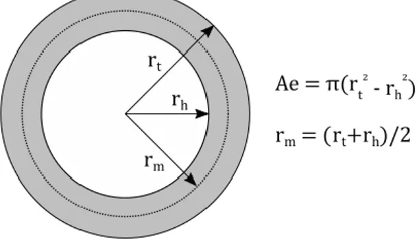
The axial compressor and turbine can have several stages, but from the cycle simulation only the component inlet and outlet are known. As first step the total and static state at each stage inlet and outlet are calculated, using the polytropic efficiency, fluid property functions and a prescribed number of stages. If the resulting pressure ratio of the first stage is too high, the number of stages is increased until it is smaller than a specified maximum value. The calculated flow area changes from stage to stage. The change in flow area is realized by varying two of the three variables inner hub radius, mean radius and outer tip radius, while keeping one (almost) constant, see figure 2. Which radius is kept constant is specified through the enumeration DesignMode.
The volume per blade, the number of blades and the blade pull stress are calculated from the radii, specified aspect ratio, volume factor, solidity and taper ratio. The blade pull stress is then the main input for estimating the disc thickness. The WATE-2 report gives the relation between blade pull stress and thickness as a graph. This graph has been converted into a table and a function that interpolates between the table values.
Selected details of the implemented weight estimation methods have been shown. Complete details are available from [29,30]. We consider the use of a fully documented weight estimation methodology as a key advantage over using non-transparent proprietary methods. Through object-orientation,
this baseline methodology can be extended and adapted to include proprietary aspects in a convenient way.
Figure 2: Flow area per stage, and the three radii that can be specified as constant depending on DesignMode. Weight estimation methods have also been implemented for the following components and sub-components:
• Compressor and turbine (blades, stator, disc, hardware, case frame)
• Duct and burner, • Shafts,
• Mixer, • Splitter, • Nozzle.
The overall weight of all components is then collected and summed up using inner and outer variables (“dynamic scoping” in Modelica parlance). Weight estimation can be turned on or off globally using an enumeration.
Naming convention
Instead of applying a new naming convention for variables, the existing naming convention from SAE ARP 5571 is applied [34].
UNMIXED TURBOFAN CYCLE/WEIGHT ANALYSIS This section introduces the first of the two application examples. It describes the system model of an unmixed flow two-spool turbofan and presents a comparison against published reference cycle results generated from NPSS and weight estimation results from WATE++.
JT9D System Model
The JT9D engine is a high bypass ratio jet engine for commercial wide-body aircraft first operated in the 1970s. It consists of an airbreathing gas turbine core and adds on an air intake, exhaust nozzle and a fan with secondary nozzle for flow bypassing the core. Using Modelon JPL, and the mentioned Modelica design patterns, a modular system model was developed for the JT9D. Several days of effort went into the model setup. In terms of abstract model topology and parameterization it matches exactly the NPSS model of the same engine published by [35] and available online from [36]. The model topology matches this NPSS reference model only in the
abstract sense as there exists a one-to-one mapping between component models in the NPSS model, and component models in the JPL-based model, but the latter uses additional hierarchy levels for structuring the gas turbine model to facilitate reuse. With Modelica technology and JPL, models can also be built on a “flat” hierarchy level like the NPSS model but the layered architecture approach was favored for the particular model discussed here.
Figure 3a: On-design comparison of mass flow rates
Figure 3b: On-design comparison of total pressures
The subsystems are instantiated within a template model for the engine and are replaceable, enabling the flexibility to compose any unique system with the same architecture. Subsystems are built from partial model classes that define the
Figure 3c: On-design comparison of total temperatures
required interfaces to be used within the engine model. The subcomponents that build up the subsystems are developed to be used for both on-design and off-design calculations.
The engine model begins with an ambient air source that feeds into the first subsystem, the inlet, that takes in ram air and determines the pressure from a pressure recovery model and pressure loss models. Second is the compressor subsystem, which is composed of a fan, low pressure compressor (LPC) and HPC. Between the fan and the compressors is a splitter which diverts the bypass flow to a secondary nozzle. The main air flow continues to the combustor, which mixes fuel into the air for combustion to heat the air. Then, the combusted gas expands through a turbine subsystem with high and low pressure turbine sections. Lastly, the system ends with the primary nozzle to determine the generated thrust. The last subsystem is the shafts block that connects the mechanical interfaces of the compressors and turbines. This uses a vectorized mechanical shaft connector for flexibility in modeling engines with different numbers of spools. Here, the respective components are connected on the low pressure and the high-pressure spool indices (1 and 2). An additional entry in the vector of mechanical shaft connectors is available to define how the fan is connected to the spools. In this case, a direct drive through the low-pressure spool is modeled, and component 3 is directly connected to component 1. Additional mechanical models such as bearing or thermal losses can be included here but were not required based on the reference NPSS model.
The comparison model built with JPL uses the same performance maps and “Lagrange2”-type map interpolation. The fan is modeled with a single performance map (no distinction between inner and outer streams). Four bleed flows are extracted from the HPC based on user-defined flow fractions, pressure, and work fractions. Two flows are each routed to the high pressure turbine (HPT) and low pressure turbine (LPT) for
-0,07% -0,06% -0,05% -0,04% -0,03% -0,02% -0,01% 0,00% 0,01% 0 100 200 300 400 500 600 700 800 FS _1 FS _21 FS _22 FS _24 FS_3 FS_4 FS _48 FS_7 FS _15 FS _19 re lat iv e d ev iat ion m ass f low in k g/s NPSS JPL dev_rel -1,0% -0,8% -0,6% -0,4% -0,2% 0,0% 0 5 10 15 20 25 re lat iv e d ev iat ion p re ss u re in b ar NPSS JPL dev_rel -0,6% -0,5% -0,4% -0,3% -0,2% -0,1% 0,0% 0,1% 0,2% 0 200 400 600 800 1000 1200 1400 1600 FS _1 FS _21 FS _22 FS _24 FS_3 FS_4 FS _48 FS_7 FS _15 FS _19 re lat iv e d ev iat ion tem p era tu re in K NPSS JPL dev_rel
cooling. Here, a distinction is made on whether the cooling flows contribute to the turbine work or not (all cooling flows are configured to partially contribute to turbine work, after subtracting pumping power, but then pumping power is set to zero, and the cooling flows are injected at turbine inlet and turbine outlet pressures respectively, which represents the contribution to turbine work in the NPSS JT9D model). Cycle results comparison against NPSS
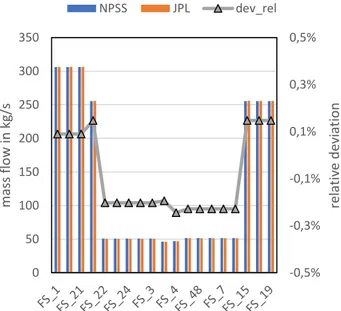
The comparison against NPSS results is done by plotting values for mass flow, total pressure and total temperature along the flow path for NPSS and JPL, as well as the relative deviation. The exact positions being compared have flow station numbers according to ARP 755. This convention leaves some room for interpretation, and the flow station definitions used in the NPSS JT9D model are used in this comparison. JPL default station names are overridden for the comparison.
For the on-design case, the comparison is shown in figure 3. This is “case 0” in the original data set. Agreement is very good, the maximum difference for all values is below 1%, with the average difference being much smaller. The most reasonable explanation for the observed deviations is via differences in the thermodynamic properties. In the given model setup, NPSS uses thermodynamic properties based on table look-up following [37] (“GasTbl”). The Modelica-based solution implements the polynomial equations of [23] for specific heat capacity 𝑐𝑝, specific enthalpy ℎ, specific entropy 𝑠, temperature-dependent part of specific entropy 𝑠0, gas constant 𝑅, isentropic exponent 𝛾, dynamic viscosity 𝜂. Additionally, a fully rigorous conversion between static and total quantities suggested by Sethi [25] is used. Additionally to potential differences due to thermodynamic property implementations, NPSS results in text files are truncated to a limited number of significant digits. The rounding error is in the same order of magnitude as the deviation shown in the figures. The differences in thermodynamic properties
Figure 4a: Off-design comparison of mass flow rates
Figure 4b: Off-design comparison of total pressures
Figure 4c: Off-design comparison of total temperatures may therefore even be negligible.
For the off-design case (case number 807 in the original data set), the comparison is shown in figure 4. Here, we observe somewhat larger differences, between approximately 0% and 1.4% (between 0.2% and 0.4% on average). Again, we assume these to be caused by the thermodynamic property routines, round-off error, and/or minor inconsistencies in the model setup. Weight estimation results comparison against WATE++
The comparison against WATE++ results for compressors and turbines is done in a similar manner, by plotting values along
-0,5% -0,3% -0,1% 0,1% 0,3% 0,5% 0 50 100 150 200 250 300 350 re lat iv e d ev iat ion m ass f low in k g/s NPSS JPL dev_rel -2% -1% 0% 1% 2% 0 1 2 3 4 5 6 7 8 9 10 re lat iv e d ev iat ion p re ss u re in b ar NPSS JPL dev_rel -0,5% -0,3% -0,1% 0,1% 0,3% 0,5% 0 200 400 600 800 1000 1200 1400 1600 FS _1 FS _21 FS _22 FS _24 FS_3 FS_4 FS _48 FS_7 FS _15 FS _19 re lat iv e d ev iat ion tem p era tu re in K NPSS JPL dev_rel
the flow path. Exemplarily selected results are shown for the HPC in figure 5.
Figure 5a: Compressor pressure ratio per stage
Figure 5b: Compressor flow area per stage
The pressure ratio and required flow area are decreasing along the flow path. Results show very good agreement; the deviation is less than 0.1%.
Based on the required flow area, radii and stage lengths are calculated and then masses are estimated based on empirical correlations. Results for the blade mass are shown as an example in figure 6. Other subcomponents like stator, case or connecting hardware are also calculated for each stage.
Agreement for blade mass results is very good for all stages (less than 0.8% deviation). Our implementation of WATE-2 mimics WATE++ in allowing to use a different material for the last few stages. When switching to the other material, a step in the blade masses appears (see stages 9 and 10 in figure 6).
For most of the mass estimates, for which WATE++ comparison data is available, the match is good. This holds for instance for the components that do not have stages and the result
is a single value for the mass such as ducts or the burner. For axial compressors and turbines, we observe substantial deviations.
Figure 6: Compressor blade mass per stage
Table 2 shows that the WATE-2 method estimates other total masses for axial compressors and turbines than WATE++. For LPC, HPC, and LPT we observe substantial total differences, and even more on component level (these alleviate each other however to some extend). The differences on the HPT are so large that one method must be off substantially in relation to the true mass.
For axial compressors we observe that blade mass, hardware mass, and case mass are consistently estimated between both methods. The largest deviations for the compressor are currently seen for disc mass: WATE-2 describes two possible implementations, a simple graph-based method and an advanced method that does a preliminary sizing of the disc. The current implementation uses the simpler of the two approaches, but WATE++ results are based on a variant of the advanced method. Also, the stator mass estimates differ between both methods. When the WATE++ method was developed, improvements in these areas were likely a main objective. For completeness, two additional mass items appear in WATE++ output, rotor drum and stator support flange. These are not included in table 2.
For the axial turbines, the differences in component mass estimates are even larger. Likely, a substantially changed methodology was implemented in WATE++. We assume that this leads to more appropriate estimates but recognize that the LPT total mass estimate from WATE-2 still matches that of WATE++ rather closely. The HPT results require substantial improvements, also on total turbine mass estimate. For completeness, we again highlight that WATE++ output contains additional mass items vane flange, rotor drum, rub strip, rotor shroud, vane shroud, case cooling, interstage seal, and space bar (depending on turbine). These are not included in table 2.
-0,06% -0,04% -0,02% 0,00% 0,02% 0,04% 1 1,05 1,1 1,15 1,2 1,25 1 2 3 4 5 6 7 8 9 10 11 re lat iv e d ev iat ion p re ss u re ra tio HPC stages WATE++ JPL err_rel -0,100% -0,075% -0,050% -0,025% 0,000% 0,025% 0,050% 0 0,05 0,1 0,15 0,2 0,25 0,3 1 2 3 4 5 6 7 8 9 10 11 re lat iv e d ev iat ion flow ar ea in m² HPC stages WATE++ JPL err_rel -5% 0% 5% 0 5 10 15 20 25 1 2 3 4 5 6 7 8 9 10 11 re lat iv e erro r b lad e mas s in k g HPC stages
Group Component WATE++ WATE-2 err_rel kg kg - LPC Total 196 225 15% Blades 18 18 0% Stators 58 35 -40% Disc 66 119 80% Case 38 38 0%
Nuts and bolts 15 15 0%
HPC Total 564 498 -12%
Blades 114 114 0%
Stators 143 124 -13%
Disc 188 141 -25%
Case 99 99 0%
Nuts and bolts 20 20 0%
HPT Total 688 295 -57%
Blades 141 55 -61%
Vanes 204 56 -73%
Disc 172 20 -89%
Case 32 27 -14%
Nuts and bolts 6 5 -13%
Frame 134 132 -2% LPT Total 602 626 4% Blades 138 130 -6% Vanes 99 172 73% Disc 144 83 -42% Case 67 58 -13%
Nuts and bolts 12 10 -13%
Frame 141 171 21%
Table 2: Mass estimates of WATE-2 and WATE++ BOOSTED TURBOFAN CYCLE ANALYSIS
Conventional high bypass ratio turbofan engines are either affected by reduced efficiency due to higher aerodynamic loading or higher weight from increased number of stages for booster and low-pressure turbine [38]. Furthermore, for such designs, the requirement for maintaining a lower fan tip speed limits the rotational speed of the low-pressure shaft. Introduction of a gearbox can relieve this issue by permitting the design of these two components at their optimal speeds, whilst maintaining the aerodynamic loading with a lower number of stages to achieve good efficiency and thus reduce the weight [39,1]. This section describes a comparison with the cycle performance tool EVA [40,41] on such a geared turbofan. The underlying model is described in more detail in [42], and used there for an analysis of hybridization strategies.
Boosted Turbofan System Model
A geared turbofan (GTF), is a two and half shafts engine. The core of the GTF engine comprises an intake, three compressors: a fan, a HPC and an intermediate pressure compressor (IPC), a combustor, two turbines: a HPT, and a LPT and core nozzle and bypass nozzle. The high-speed shaft (HPS) links the HPT and the HPC. The LPT drives the fan through a gearbox and the one and half shafts. The parallel hybrid set up is achieved through coupling of an accessory gearbox to the low-pressure shaft at one end and electrical motor on the other end, in similar way as designed for power off-take in conventional engine. Such arrangement enables electrical power assistance for varying range, additionally or in-lieu-of the gas turbine engine for driving the propulsor unit. The electrical motor in the back end is connected to a power converter system and battery for drawing of the electrical energy.
The intake of the engine captures the free stream and is used for calculating the total conditions and momentum drag. The outlet total pressure is then calculated assuming a certain level of pressure losses as a function of the flight Mach number.
In the fan component, separate characteristics are used for the fan core and fan bypass. The larger part of the airflow bypasses the core of the engine and goes through a bypass duct to finally get ejected through a convergent nozzle. The air flow through the fan core passes through the IPC and subsequently through the HPC, wherein it gets compressed through multiple stages. With the increased pressure, the air enters the combustion chamber, and is mixed with jet fuel. The high-energy air mass leaves the combustor and then expands through HPT, and LPT. After expanding in both the turbines, the fluid flow is directed to the nozzle where it is finally exhausted to the atmospheric condition through the core nozzle.
Handling bleed is only used for the flight and ground idle operating points, as well for approach operation. It is scheduled to be extracted from IPC component. The required customer bleed flow may be extracted either from the IPC or the HPC component. The actual extraction amount is dependent on the flight altitude. The HPT cooling flow is scheduled to be extracted from the HPC outlet, out of which a fraction of the flow is diverted to do work in the rotor. The LPT cooling flow is extracted before the full compression process in the HPC and only a part of it is considered to do work in the rotor. Nozzle Guide Vanes (NGV) and blades, as well as sealings are considered to be supplied with cooling flow both for HPT and LPT. The LPT sealing and outlet casing flows are extracted at the early stage of HPC compression process; a part of the former is considered to do work in the rotor. For the burner component combustion efficiency is considered based on combustor load and volume. The fraction of the turbine cooling air that does work in the rotor is mixed with the turbine main inlet flow at the rotor inlet and the rest is mixed at the outlet of the turbine rotor. The latter portion of the cooling air is therefore not considered in the efficiency calculation. For the core flow and the bypass flow, fixed area convergent nozzle components are used. A fixed
mechanical efficiency is assumed for the HPS, fan shaft, and LPS components.
Again, several days of effort went into creating a comparison model in JPL. The comparison model uses the same performance maps and linear map interpolation (while JPL also supports Lagrange2, Lagrange3, and Akima, this is the algorithm used by EVA). Four bleed flows are extracted from the HPC based on a computation of required flows to ensure a specific blade temperature via the blade cooling model of Kurzke [43] (a specific parameterization of the model suggested by Horlock [44]). JPL currently only offers a different, somewhat more sophisticated blade cooling model (model A of [45,46]). To avoid inconsistent cooling flows, it was therefore decided to use the bleed/cooling flows computed by EVA also in the JPL model. Instead of computing the cooling flows in JPL, we therefore computed resulting uniform blade temperatures. Again, a distinction is made on whether the cooling flows contribute to the turbine work or not (no cooling flow is configured to partially contribute to turbine work after subtracting pumping power; instead, they are simply configured to fully contribute to turbine work, or to contribute not at all).
Cycle results comparison against EVA
The comparison against EVA results is again illustrated by plotting values for mass flow, total pressure and total temperature along the flow path for EVA and JPL, as well as the relative deviation. Again, the flow station definitions used in the reference model are used in this comparison (EVA in this case). JPL default station names are overridden for the comparison.
For the on-design case, the comparison is shown in figures 7. Agreement is good; the maximum difference for all values is below 3.5%, with the average difference being 0% to 2%. There are a few likely explanations for the observed deviations. First, JPL uses different thermodynamic property routines in comparison to EVA. In the latter, thermodynamic properties are
Figure 7a: On-design comparison of mass flow rates
Figure 7b: On-design comparison of total pressures
Figure 7c: On-design comparison of total temperatures
obtained from fluid tabulations. The data are mainly generated by CEA [47] and Walsh and Fletcher fluid model [23]. Alternatively, polynomial libraries in CHEMKIN-II format [48] can be utilized in EVA to study the feasibility of any working fluid and alternative fuel. More details about the fluid model implemented in EVA can be found in [49-51].
Additionally to the differences in thermodynamic properties, at the time of writing, JPL does not apply the classic compensation of performance maps with respect to Reynolds Number Index [33], which has relevant influence at the simulated “top of climb” conditions. EVA and JPL do apply the
-0,04% -0,03% -0,02% -0,01% 0,00% 0,01% 0,02% 0 20 40 60 80 100 120 140 160 180 FS _2 FS _24 FS _26 FS _31 FS _41 FS _43 FS _45 FS_6 FS _13 FS _18 re lat iv e d ev iat ion m ass f low in k g/s EVA JPL dev_rel -0,50% 0,00% 0,50% 1,00% 1,50% 2,00% 2,50% 3,00% 3,50% 4,00% 0 5 10 15 20 25 re lat iv e d ev iat ion p re ss u re in b ar EVA JPL dev_rel -0,10% 0,00% 0,10% 0,20% 0,30% 0,40% 0,50% 0,60% 0,70% 0,80% 0,90% 0 200 400 600 800 1000 1200 1400 1600 1800 2000 FS _2 FS _24 FS _26 FS _31 FS _41 FS _43 FS _45 FS_6 FS _13 FS _18 re lat iv e d ev iat ion tem p era tu re in K EVA JPL dev_rel
same model for pressure losses due to cooling air mixing in the turbine however. This model for mixing pressure losses is based on Hartsel [52] and Horlock [53]. It relies on the following pressure loss equation.
Δ𝑝0 𝑝0
= 𝑘𝜓 (6)
The total pressure loss Δ𝑝0, normalized by the inlet total pressure 𝑝0, is the product of a small constant 𝑘 and the ratio of cooling to inlet gas mass flow rate 𝜓. The constant 𝑘 is set to is 0.1 for nozzle guide vane cooling and 0.2 for rotor cooling.
Figure 8a: Off-design comparison of mass flow rates
Figure 8b: Off-design comparison of total pressures
Figure 8c: Off-design comparison of total temperatures
A comparison of off-design results for a take-off case are shown in figure 8. The match is again good and the deviations are similar to those of the discussed on-design results (0% to approximately 3.5% relative error).
CONCLUSIONS
The open standards Modelica and FMI are a feasible choice for gas turbine system modeling and simulation. Design patterns were defined to solve special gas turbine simulation problems such as on-design vs. off-design. Using JPL, the leading Modelica library for gas turbine applications, we showed that high quality results on par with domain specific simulation codes can be generated. At the time of writing, some result differences in cycle performance and weight estimation are still evident. These have to be analyzed and eliminated with evolutionary improvements to thermodynamic property modeling, and additional component modeling detail such as Reynold’s Number Indexing or turbine cooling mixing loss models. In the area of gas turbine mass estimates, a further analysis and extension of openly published methods would be desirable. Following the results of this work, the quality and completeness of these is still inferior to proprietary methods.
Overall, these results show that the ambition to design and analyze alterative propulsion concepts using modeling and simulation technology used across different engineering domains is feasible. Like this, it is possible to avoid implementing full design and analysis capability for other engineering domains than gas turbines such as electrical power systems or closed supercritical cycles in domain-specific gas turbine modeling and simulation technology. Mature and complete solutions for many engineering domains can now be coupled together in a powerful way using layered architectures. It is our hope that openly available methodologies and standards
-2,50% -2,00% -1,50% -1,00% -0,50% 0,00% 0 50 100 150 200 250 300 350 400 450 FS _2 FS _24 FS _26 FS _31 FS _41 FS _43 FS _45 FS_6 FS _13 FS _18 re lat iv e d ev iat io n m ass f low in k g/s EVA JPL dev_rel -3,00% -2,00% -1,00% 0,00% 1,00% 2,00% 3,00% 4,00% 0 10 20 30 40 50 60 re lat iv e d ev iat ion p re ss u re in b ar EVA JPL dev_rel 0,00% 0,50% 1,00% 1,50% 2,00% 2,50% 3,00% 3,50% 4,00% 0 500 1000 1500 2000 2500 FS _2 FS _24 FS _26 FS _31 FS _41 FS _43 FS _45 FS_6 FS _13 FS _18 re lat iv e d ev iat ion tem p era tu re in K EVA JPL dev_rel
accelerate innovation. This could be tremendous value looking at the current speed of innovation in engineering simulation. ACKNOWLEDGMENTS
We would like to thank the anonymous reviewers for their improvement suggestions. These strongly improved the quality of this article.
Some of the work described in this article was executed as part of the project Turbo electRic Aircraft Design Environment (TRADE), which has received funding from the Clean Sky 2 Joint Undertaking under the European Union’s Horizon 2020 Research and Innovation Programme under Grant Agreement number 755458. The project team recognizes that current aircraft/engine conceptual design methodologies are centered on the disciplines of aerodynamics, structures, and gas turbine performance. Key aspects of unconventional concepts - such as hybrid electric propulsion - are thus hard to capture within existing design tools. TRADE proposes the integration of three new aspects into aircraft/engine conceptual design. First, an advanced structural model quantifies the impact of the installation of heavy equipment on the sizing of the aircraft structure. Second, refined onboard system models capture design and performance trades in electric power systems, gas turbines, and thermal management. Finally, an operational and mission model enables flight dynamic analyses of diverging aircraft configurations. TRADE also delivers the integration of these new aspects into a conceptual design environment. The environment is suitable for the design of hybrid electric aircraft. First configuration assessment and optimization results for a boosted turbofan (parallel hybrid) are available in Zhao et al. [42,54].
REFERENCES
[1] K. G. Kyprianidis, A. M. Rolt, and T. Grönstedt, "Multidisciplinary analysis of a geared fan intercooled core aero-engine," Journal of Engineering for Gas Turbines and Power, vol. 136, no. 1, p. 011203, 2014.
[2] Michael Winter. A view into the next generation of commercial aviation (2025 timeframe). In AIAA Aerospace Today and Tomorrow, 2013.
[3] Linda Larsson, Tomas Grönstedt, and Konstantinos G Kyprianidis. Conceptual design and mission analysis for a geared turbofan and an open rotor configuration. In ASME 2011 Turbo Expo: Turbine Technical Conference and Exposition, pages 359–370. American Society of Mechanical Engineers, 2011.
[4] DeServi, C.M.; Azzini, L.; Pini, M.; Gangoli Rao, A.; Colonna, P. Exploratoy Assessment of a combined-cycle engine concept for aircraft propulsion. In Proceedings of the 1st Global Power and Propulsion Forum, Zurich,
Switzerland, 16–18 January 2017; p. 11.
[5] M. K. Bradley, C. K. Droney, Subsonic Ultra Green Aircraft Research: Phase II – Volume II – Hybrid Electric Design Exploration, NASA/CR–2015-218704.
[6] J. Welstead, J. L. Felder, Conceptual Design of a Single-Aisle Turboelectric Commercial Transport with Fuselage
Boundary Layer Ingestion, in: 54th AIAA Aerospace Sciences Meeting, San Diego, CA, 2016.
[7] J. L. Felder, G. V. Brown, H. D. Kim, J. Chu, Turboelectric Distributed Propulsion in a Hybrid Wing Body Aircraft, in: 20th International Symposium on Air Breathing Engines (ISABE), Gothenburg, Sweden, 2011
[8] S. M. Jones, “Steady-State Modeling of Gas Turbine Engines Using the Numerical Propulsion System Simulation Code”, GT2010-22350, 2010.
[9] J. Lytle, G. Follen, C. Naiman, and A. Evans, "Numerical propulsion system simulation (NPSS) 1999 industry review," 2000.
[10] R. W. Claus, A. Evans, J. Lylte, and L. Nichols, "Numerical propulsion system simulation," Computing Systems in Engineering, vol. 2, no. 4, pp. 357-364, 1991.
[11] J. Kurzke, “Advanced User-Friendly Gas Turbine Performance Calculations on a Personal Computer”, ASME 95-GT-147, 1995.
[12] J. Kurzke, “Transient Simulations During Preliminary Conceptual Engine Design”, ISABE 2011-1321, 2011. [13] Visser, W.P.J. and Broomhead M.J., 2000, “GSP, A Generic
Object Oriented Gas Turbine Simulation Environment”, ASME-2000-GT-0002, also NLR-TP-2000-26
[14] A. Bala, V. Sethi, E. Lo Gatto, V. Pachidis, and P. Pilidis, "PROOSIS—A Collaborative Venture for Gas Turbine Performance Simulation Using an Object Oriented Programming Schema," ISABE 2007 Proceedings, ISABE, vol. 1357, 2007.
[15] Modelica Language Specification 3.4,
https://modelica.org/documents/, accessed Oct 2018. [16] Åström, Elmqvist, Mattsson: Evolution of continuous-time
modeling and simulation. Proceedings of the 12th European Simulation Multiconference on Simulation-Past, Present and Future, pp. 9-18, 1998.
[17] Functional Mock-Up Interface 2.0 for Model Exchange and Co-simulation, https://fmi-standard.org/, accessed Oct 2018.
[18] Blochwitz T., Otter M., Arnold M., Bausch C., Clauß C., Elmqvist H., Junghanns A., Mauss J., Monteiro M., Neidhold T., Neumerkel D., Olsson H., Peetz J.-V., Wolf S. (2011): “The Functional Mockup Interface for Tool independent Exchange of Simulation Models”, 8th International Modelica Conference, Dresden 2011.
[19] Blochwitz T., Otter M., Akesson J., Arnold M., Clauß C., Elmqvist H., Friedrich M., Junghanns A., Mauss J,, Neumerkel D., Olsson H., Viel A. (2012): Functional Mockup Interface 2.0: The Standard for Tool independent Exchange of Simulation Models”, 9th International Modelica Conference, Munich, 2012.
[20] M. Tiller, “Modelica by Example”,
http://book.xogeny.com/, accessed Oct 2018.
[21] M. Tiller, “Introduction to Physical Modeling with Modelica”, Kluwer Academic Publishers, 2001.
[22] P. Fritzson, “Principles of Object-Oriented Modeling and Simulation with Modelica 3.3: A Cyber-Physical Approach”, Wiley, 2015.
[23] P. P. Walsh, P. Fletcher, “Gas Turbine Performance”, second edition, Blackwell Publishing, 2004.
[24] J. Kurzke, “About simplifications in gas turbine performance calculations”. In Proceedings of the ASME Turbo Expo, volume 3, pages 14–17, May 2007.
[25] V. Sethi, “Advanced performance simulation of gas turbine components and fluid thermodynamic properties”, PhD thesis, Cranfield University, April 2008
[26] H. Elmqvist, H. Tummescheit, M. Otter, “Object-oriented modeling of thermo-fluid systems”. In Proceedings of the Third International Modelica Conference, pages 269–286, Linköping, Sweden, 2003.
[27] R. Schaber. Numerische Auslegung und Simulation von Gasturbinen. PhD thesis, Lehrstuhl für Flugantriebe, Technische Universität München, December 2000.
[28] Lolis 2014: Development of a Preliminary Weight Estimation Method for Advanced Turbofan Engines, Cranfield University 2014.
[29] R. J. Pera. E. Onat. G. W. Klees, E. Tjonneland: “A Method to Estimate Weight and Dimensions of Aircraft Gas Turbine Engines”, NASA-CR-135170, 1977.
[30] E. Onat, G. W. Klees: “A method to estimate weight and dimensions of large and small gas turbine engines”, NASA-CR-159481, 1979.
[31] M. T. Tong, I. Halliwell, L. J. Ghosn, “A Computer Code for Gas Turbine Engine Weight and Life Estimation,” ASME Journal of Engineering for Gas Turbine and Power, 2004. [32] M.T. Tong, B. A. Naylor, “An Object-Oriented Computer
Code for Aircraft Engine Weight Estimation,” GT2008-50062, ASME TurboExpo, 2008.
[33] J. Kurzke, I. Halliwell: “Propulsion and Power”, Springer International Publishing, 2018.
[34] Anon.: “Gas turbine engine performance presentation and nomenclature for digital computers using object-oriented programming”, ARP5571, Society of Automotive Engineers, 200
[35] Jeffryes W. Chapman, Thomas M. Lavelle, Ryan D. May, Jonathan S. Litt and Ten-Huei Guo: Toolbox for the Modeling and Analysis of Thermodynamic Systems (T-MATS) User’s Guide. NASA Technical Memorandum 2014-216638, 2014.
[36] Anon.: “An open source thermodynamic modeling package completed on behalf of NASA”, https://github.com/nasa/T-MATS, accessed Oct 2018.
[37] S. Gordon, Thermodynamic and Transport Combustion Properties of Hydrocarbons With Air, NASA Technical Paper 1906, July 1982.
[38] J. Kurzke, "Fundamental differences between conventional and geared turbofans," in ASME Turbo Expo 2009: Power for Land, Sea, and Air, 2009, pp. 145-153: American Society of Mechanical Engineers.
[39] K. G. Kyprianidis and A. M. Rolt, "On the optimisation of a geared fan intercooled core engine design," in ASME Turbo Expo 2014: Turbine Technical Conference and Exposition, 2014, pp. V03AT07A018-V03AT07A018: American Society of Mechanical Engineers.
[40] K. G. Kyprianidis, "Multi-disciplinary conceptual design of future jet engine systems," 2010.
[41] K. G. Kyprianidis, "An Approach To Multi-Disciplinary Aero Engine Conceptual Design," presented at the 23rd International Society for Air Breathing Engines Manchester, UK, 2017.
[42] X. Zhao, S. Sahoo, K. Kyprianidis, J. Rantzer, M. Sielemann “Off-design performance analysis of hybridized aircraft gas turbine”, submitted to ISABE 2019.
[43] J. Kurzke, "Achieving maximum thermal efficiency with the simple gas turbine cycle." 9th CEAS European Propulsion Forum: Virtual Engine—A Challenge for Integrated Computer Modelling, Rome, Italy, Oct. 2003.
[44] J. H. Horlock, D. T. Watson, T. V. Jones, Limitations on Gas Turbine Performance imposed by Large Turbine Cooling Flows, ASME 2000-GT-635, 2000
[45] K. Jordal, L. Torbidoni, A. F. Massardo: "Convective Blade Cooling Modelling for the analysis of innovative gas tuerbine cycles", 2001-GT-0390, ASME Turbo Expo 2001 [46] L. Torbidoni, A. F. Massardo: "Analytical Blade Row
Cooling Model for Innovative Gas Turbine Cycle Evaluations Supported by Semi-Empirical Air-Cooled Blade Data", ASME Transactions 2004
[47] McBride, B.J., Gordon, S., and Reno, M. A., 1993,‘‘Coefficients for calculating thermodynamic and transport properties of individual species’’, NASA Technical Memorandum 4513.
[48] Kee, R.J., Rumpley, F.M., and Miller, J.A., 1992, “The Chemkin Thermodynamic Data Base”, Sandia National Laboratories, Report No. SAND-8215B.
[49] Kyprianidis, Konstantinos & Sethi, Vishal & Ogaji, Stephen & Pilidis, Pericles & Singh, Riti & Kalfas, Anestis. (2009). Thermo-Fluid Modelling for Gas Turbines-Part I: Theoretical Foundation and Uncertainty Analysis. Proceedings of the ASME Turbo Expo. 4. 10.1115/GT2009-60092.
[50] Kyprianidis KG, Sethi V, Ogaji ST, Pilidis P, Singh R, Kalfas AI. Thermo-Fluid Modelling for Gas Turbines—Part II: Impact on Performance Calculations and Emissions Predictions at Aircraft System Level. ASME. Turbo Expo: Power for Land, Sea, and Air, Volume 4: Cycle Innovations; Industrial and Cogeneration; Manufacturing Materials and Metallurgy; Marine ():483-494. doi:10.1115/GT2009-60101.
[51] Kyprianidis, Konstantinos & Sethi, Vishal & Ogaji, SOT & Pilidis, Pericles & Singh, Riti & Kalfas, Anestis. (2012). Uncertainty in gas turbine thermo-fluid modelling and its impact on performance calculations and emissions predictions at aircraft system level. Proceedings of the Institution of Mechanical Engineers, Part G: Journal of Aerospace Engineering. 226. 163-181. 10.1177/0954410011406664.
[52] J. Hartsel. "Prediction of effects of mass-transfer cooling on the blade-row efficiency of turbine airfoils", 10th Aerospace Sciences Meeting, Aerospace Sciences Meetings, https://doi.org/10.2514/6.1972-11
[53] Horlock JH. The Basic Thermodynamics of Turbine Cooling. ASME. J. Turbomach. 2000;123(3):583-592. doi:10.1115/1.1370156.
[54] X. Zhao, S. Sahoo, K. Kyprianidis, S. Sumsurooah, G. Valente, M. Rashed, G. Vakil, C. Hill, C. Jacob, A. Gobbin, A. Bardenhagen, K. Prölss, M. Sielemann, J. Rantzer, E. Ekstedt, A Framework For Optimization Of Hybrid Aircraft, ASME TurboExpo 2019, GT2019-91335, June 2019.