DISSERTATION
Submitted by
In partial fulfillment of the requirements for the degree of Doctor of Philosophy
Colorado State University Fort Collins, Colorado
Doctoral Committee:
AEROSOL SINGLE-SCATTERING ALBEDO RETRIEVAL OVER NORTH AFRICA USING CRITICAL REFLECTANCE
Department of Atmospheric Science Kelley C. Wells
Jennifer Peel Jeffrey Collett Graeme Stephens
Advisor: Sonia Kreidenweis
Richard Johnson Department Head:
Fall 2010
ABSTRACT
AEROSOL SINGLE-SCATTERING ALBEDO RETRIEVAL OVER NORTH AFRICA USING CRITICAL REFLECTANCE
The sign and magnitude of the aerosol radiative forcing over bright surfaces is highly dependent on the absorbing properties of the aerosol. Thus, the determination of aerosol forcing over desert regions requires accurate information about the aerosol single-scattering albedo (SSA). However, the brightness of desert surfaces complicates the retrieval of aerosol optical properties using passive space-based measurements. The aerosol critical reflectance is one parameter that can be used to relate top-of-atmosphere (TOA) reflectance changes over land to the aerosol absorption properties, without knowledge of the underlying surface properties or aerosol loading. Physically, the parameter represents the TOA reflectance at which increased aerosol scattering due to increased aerosol loading is balanced by increased absorption of the surface contribution to the TOA reflectance. It can be derived by comparing two satellite images with
different aerosol loading, assuming that the surface reflectance and background aerosol are similar between the two days.
In this work, we explore the utility of the critical reflectance method for routine monitoring of spectral aerosol absorption from space over North Africa, a region that is predominantly impacted by absorbing dust and biomass burning aerosol. We derive the critical reflectance from Moderate Resolution Spectroradiometer (MODIS) Level 1B
reflectances in the vicinity of two Aerosol Robotic Network (AERONET) stations: Tamanrasset, a site in the Algerian Sahara, and Banizoumbou, a Sahelian site in Niger. We examine the sensitivity of the critical reflectance parameter to aerosol physical and optical properties, as well as solar and viewing geometry, using the Santa Barbara DISORT Radiative Transfer (SBDART) model, and apply our findings to retrieve SSA from the MODIS critical reflectance values. We compare our results to AERONET-retrieved estimates, as well as to measurements of the TOA albedo and surface fluxes from the Geostationary Earth Radiation Budget (GERB) experiment, Atmospheric Radiation Measurement (ARM) program, and Clouds and the Earth’s Radiant Energy System (CERES) data. Spectral SSA values retrieved at Banizoumbou result in TOA forcing estimates that agree with CERES measurements within ± 5 W m-2 for dusty conditions; however, the retrieved SSA translates to a much larger positive TOA forcing than CERES in the presence of dust-biomass burning mixtures. At Tamanrasset, the retrieval captures changes in aerosol absorption from day to day, but the SSA appears to be biased high when compared to AERONET and CERES. This may be due to the higher surface reflectance in this region, an overestimation of the dust aerosol size, or changing background aerosol between the clean and polluted day. Our retrieval results indicate that we can be most confident in the retrieved SSA for scattering angles between 120º and 160º, satellite view angles less than ~ 45º, and in cases when the background aerosol on the cleaner day is non-absorbing.
ACKNOWLEDGEMENTS
I have been so lucky to have such wonderful mentors and collaborators
throughout my time at CSU. First, I would like to thank my advisor, Sonia Kreidenweis, for her guidance and enthusiastic support of me and this project, for helping me to always find new ways to look at an existing problem, and for her warm sense of humor. Many thanks also to committee member Lorraine Remer for her endless encouragement and helpful input, and for keeping me motivated with the occasional ice cream. I am very grateful to Vanderlei Martins for the many helpful conversations and analysis tools— without his critical reflectance expertise this work would not have been possible. Thanks to committee member Graeme Stephens for his support and ideas, and for his help with numerous radiative transfer problems throughout this project. I also sincerely thank my other committee members, Jeffrey Collett and Jennifer Peel, for their expertise and help in refining this work.
Thanks to Rob Levy and Shana Mattoo for their help with the details of the MODIS operational aerosol retrieval, and to Tom Eck for his help in interpreting the AERONET data. Thanks also to Li Zhu for her suggestions on making my analysis more efficient, and for her efforts in our method comparison. Additionally, I would like to thank Didier Tanré, Emilio Cuevas-Agullo, and Mohamed Mimouni for their efforts in establishing and maintaining the Banizoumbou and Tamanrasset AERONET sites. Thanks to Ben Johnson for providing data from the DABEX campaign, and for his help
with its interpretation. I also wish to extend thanks to Mark Ringerud for help with computing and data management, and to Chris Kummerow for providing additional computing resources for this work. Furthermore, my utmost appreciation goes to everyone in the CSU Atmospheric Chemistry groups—particularly those in the
Kreidenweis group—for their support, advice, and friendship during my time at CSU and beyond. Finally, I would like to thank my family for their unyielding support, love, and encouragement throughout this work and all the years leading up to it. My sincerest thanks go especially to John for being so willing to go on this adventure with me. I would not have made it to this point without him at my side.
This work was generously supported by the Center for Earth Atmosphere Studies through NASA grant NNG06GB41G.
TABLE OF CONTENTS
1 INTRODUCTION... 1
1.1 OVERVIEW OF AEROSOL INTERACTIONS WITH RADIATION... 2
1.1.1 Definition of Optical Parameters... 2
1.1.2 Impact of Aerosols on Earth’s Energy Budget over Land ... 5
1.2 MEASURING AEROSOL ABSORPTION REMOTELY... 8
1.2.1 Geometry Considerations ... 8
1.2.2 Satellite-Based Retrievals ... 10
1.2.2.1 TOMS AI...10
1.2.2.2 DeepBlue ...11
1.2.3 Ground-Based Retrievals... 12
1.3 OVERVIEW OF AEROSOL IMPACTS IN NORTH AFRICA... 13
1.3.1 Aerosol Types and Seasonality ... 13
1.3.2 Physical and Optical Properties ... 18
1.4 CRITICAL REFLECTANCE PRINCIPLE... 21
1.4.1 Definition and Assumptions ... 21
1.4.2 Foundational Work and Applications ... 23
1.4.2.1 Demonstration of Principle...23
1.4.2.2 Saharan Dust Absorption...24
1.4.3 Other Applications of the Principle ... 25
1.4.3.1 Average Saharan Dust Absorption ...26
1.4.3.2 Aerosol Properties over Saudi Arabia...27
1.5 OBJECTIVES... 27
2 RETRIEVAL METHOD AND SENSITIVITY... 29
2.1 OBSERVATIONS... 29
2.1.1 The MODIS Instrument... 29
2.1.2 Processing MODIS Level 1B Data ... 30
2.1.2.1 Correction for Gaseous Absorption and Clouds ...31
2.1.2.2 Remapping...33
2.1.2.3 Data Fitting and Assumptions ...34
2.1.2.4 Post Processing and Error Estimation...36
2.2 FORWARD MODEL... 37
2.2.1 Radiative Transfer Model Set-Up ... 38
2.2.2 Aerosol Models and Phase Function Calculations ... 40
2.2.3 Critical Reflectance LUT Building ... 42
2.3 INVERSION... 47
2.4 LUT RESULTS:IMPLICATIONS FOR SENSITIVITY TO AEROSOL CHARACTERISTICS... 49
2.4.1 Sensitivity to Solar and Viewing Geometry... 49
2.4.2 Sensitivity to Size and Shape... 59
2.4.3 Sensitivity to Fitting Method ... 63
2.5 SENSITIVITY STUDIES IN SBDART:IMPLICATIONS FOR FORWARD MODEL UNCERTAINTIES.... 63
2.5.1 Sensitivity to Assumed Refractive Index... 63
2.5.2 Sensitivity to Varying AOD ... 66
2.5.3 Sensitivity to Vertical Stratification ... 69
2.5.4 Sensitivity to Number of Streams Used in SBDART... 71
3 CASE STUDY RESULTS ... 74
3.1 TAMANRASSET AERONETSITE... 75
3.1.1 MODIS Reflectances... 75
3.1.2 Critical Reflectance and SSA Results... 82
3.1.2.1 SSA Image Retrievals...82
3.1.2.2 Spectral SSA Retrievals near AERONET Site ...86
3.2 BANIZOUMBOU AERONETSITE... 98
3.2.1 MODIS Reflectances... 98
3.2.2 Critical Reflectance and SSA Results... 102
3.2.2.1 SSA Image Retrievals...102
3.2.2.2 Spectral SSA Retrievals near AERONET Site ...104
3.3 DISCUSSION OF CASE STUDY RESULTS... 120
3.3.1 Terra-Aqua and Three-Day Comparisons ... 120
3.3.2 SSA Relationships with Geometry... 124
4 UNCERTAINTY ANALYSIS AND FORCING ESTIMATION... 137
4.1 OBSERVATION UNCERTAINTIES... 137
4.1.1 The AOD is Constant over the Retrieval Pixel... 137
4.1.2 Surface Reflectance is Invariant between the Polluted and Clean day... 141
4.1.3 The Surface Reflectance is Lambertian... 144
4.1.4 Background Aerosol and Gases are Similar between the Polluted and Clean Day... 150
4.2 FORWARD MODEL UNCERTAINTIES... 156
4.2.1 Assumed Particle Properties... 156
4.2.1.1 Size ...156
4.2.1.2 Refractive Index and Sphericity ...163
4.2.1.3 Aerosol Properties are Independent of AOD ...166
4.2.2 Aerosol Mixtures and Vertical Stratification: 19 January 2006 Case Study ... 170
4.3 AEROSOL FORCING ESTIMATION... 175
4.3.1 Tamanrasset... 175
4.3.2 Banizoumbou ... 185
5 SUMMARY AND FUTURE WORK ... 198
5.1 KEY FINDINGS... 199
5.2 SUGGESTIONS FOR CRITICAL REFLECTANCE APPLICATION... 204
5.3 FUTURE WORK... 205
APPENDIX A LUT RESULTS AT 0.553 µM ... 216
APPENDIX B SENSITIVITY TEST RESULTS AT 0.553 µM... 253
APPENDIX C IMAGE RETRIEVALS AT 0.553 µM... 272
1 Introduction
Estimating the climate effects of atmospheric aerosol with models and remote sensing techniques has been of much interest to climate scientists in recent decades. The wealth of global datasets currently available from ground and space-borne sensors provides the possibility of quantifying the perturbation of both solar and terrestrial radiation due to particulate matter of both anthropogenic and natural origin. There have been significant advances in retrieving the physical and optical properties of aerosols from remote sensing measurements (e.g. Remer et al., 2005), and in using this
information to estimate the climate effects of aerosols in clear sky conditions over ocean. The Intergovernmental Panel on Climate Change (IPCC) 4th Assessment report indicates that there is general agreement on the effect of aerosol over ocean, and that it is of similar magnitude but opposite sign as the greenhouse gas forcing (IPCC, 2007). However, the effects of aerosols over land are not as well known (Yu et al., 2006), especially over bright land surfaces where it is difficult to separate the effects of surface and aerosol reflectance in passive spectral measurements (e.g. Kaufman et al., 1997).
Over bright land surfaces, the climate effects of aerosol can vary on a regional scale, and depend strongly on the absorption properties of the aerosol. Over dark surfaces, aerosols will cool the earth-atmosphere system, and the effect is driven solely by aerosol loading; over brighter surfaces, however, aerosols could exert a warming effect if they absorb enough radiation as to appear darker than the underlying surface
(Kaufman, 1987). Additionally, bright surfaces such as deserts can be sources of
mechanically-generated dust aerosols, which are present at sizes large enough to exert a significant longwave direct effect (e.g. Haywood et al., 2005; Zhang and Christopher, 2003). Thus, the improvement of aerosol retrievals over land, and deserts specifically, remains an important area of research for the remote sensing community.
1.1 Overview of Aerosol Interactions with Radiation
Aerosols interact with solar and (for larger particles) terrestrial radiation by both scattering and absorption. These effects are a function of the particle size and optical properties, which are dependent upon their formation mechanism and chemical make-up. The following section defines some of the parameters that are commonly used to describe the interaction of aerosol with radiation, particularly when this interaction is being sensed remotely using satellite and ground-based measurement platforms.
1.1.1 Definition of Optical Parameters
The complex refractive index contains the most fundamental information about the interaction of aerosol with radiation, as it is an intrinsic property of the aerosol composition. It varies as a function of the wavelength of incident light, and is defined as:
ik n
m= − (1.1)
where n is the real part of the refractive index, and k is the imaginary part of the
refractive index. Both quantities are unitless. The real part of the refractive index is the ratio of the speed of light in a vacuum to the speed of light through the medium of
The imaginary part of the refractive index indicates the amount of absorption that occurs when light interacts with the medium.
The aerosol extinction coefficient, bext, is a function of the complex refractive
index, as well as the particle size and wavelength of incident light. It has units of inverse length (m-1), and is defined for a population of particles of varied sizes as:
∫
= minmax ( , ) ( ) 4 ) ( 2 p p D D ext p p p ext Q m x n D dD D bλ
π
(1.2)where Dp is the particle diameter, n(Dp) is the number concentration of particles of a size
Dp (cm-3), and Qext is the dimensionless extinction efficiency, which is a function of the
complex refractive index and the aerosol size parameter (x = πDp/λ). Dminp and Dmaxp
represent the upper and lower limits of the aerosol size distribution, respectively. The extinction coefficient represents the sum of the scattering and absorption coefficients (bscat + babs).
The single-scattering albedo (SSA) describes the relative effects of scattering and absorption by an aerosol population. It has no units, as it is simply the ratio of the
scattering to extinction coefficients:
ext scat
b b
SSA = (1.3)
Thus, a SSA value of 1.0 corresponds to a purely-scattering aerosol, and lower values correspond to aerosol that absorbs some fraction of incoming radiation. SSA values in this document will typically represent integrated values. Typical
column-integrated visible SSA values in the atmosphere range from ~0.7 for urban aerosol with a high black carbon content to close to 1.0 for sulfate-dominated aerosol.
The aerosol optical depth (AOD) is the most common parameter derived from satellite measurements of aerosol radiative effects, as it is a simple, unitless measure of the total column aerosol extinction. It is often represented by a lowercase tau and is defined as the vertically-integrated aerosol extinction coefficient from the surface to the top-of-atmosphere (TOA):
∫
⋅= TOA ext
a 0 b (z) dz
τ
(1.4)The scattering phase function, P(Θ), describes the angular intensity of light scattered by a population of particles. It is unitless, as it is normalized by the integrated scattered intensity over all angles:
∫
Θ Θ Θ Θ = Θ π 0 ( )sin ) ( ) ( d I I P (1.5)where I(Θ) is the intensity at scattering angle Θ. The scattering angle is defined with respect to the incoming radiation, so that Θ = 0º represents the forward scattering direction, and Θ = 180º represents the backscattering direction. Because it is dependent on the aerosol refractive index, the scattering phase function varies with wavelength, as well as particle size.
Another parameter commonly derived from remotely-sensed observations is the Angstrom exponent, α. The Angstrom exponent describes the wavelength dependence of the aerosol extinction, such that
α
λ−
≈
ext
b (1.6)
The angstrom exponent can be calculated from two measures of the extinction coefficient, or AOD, at two different wavelengths using Equation 1.7:
− = 2 1 log log 2 1
λ
λ
α
ext ext b b (1.7)Values of α generally range from 3 to 4 for very small particles, and from 0 to 1 for coarse particles (Eck et al., 1999). The presence of very large particles can result in α values that are less than 0.
The role of aerosols in the earth’s energy budget will be discussed in more detail in the following section, so we will simply define the most common terms used to describe aerosol climate effects here. The direct climate forcing of aerosols at TOA is simply defined as the change in the radiative flux (W m-2) at TOA:
↑
↑ −
=
∆FTOA Fclear Faer (1.8)
where Fclear is the upwelling flux in the absence of aerosol, and Faer is the upwelling flux
over the aerosol plume. The climate forcing of aerosols at the surface is simply defined as the difference between the fluxes incident on the surface in polluted and clean conditions:
↓
↓ −
=
∆FSFC Faer Fclear (1.9)
The forcing efficiency of aerosols is sometimes used in lieu of the forcing to describe the effect of aerosols that is independent of their atmospheric loading:
a F E τ ∆ = (1.10)
1.1.2 Impact of Aerosols on Earth’s Energy Budget over Land
The total upward radiance, I (W m-2 sr-1), at the top of the Earth’s atmosphere contains contributions from both the atmosphere and the underlying surface. Figure 1.1 shows the components of the upward radiance above an atmosphere containing aerosol
(and gases) with a reflecting surface below. Beam 1 represents the contribution from aerosol and gaseous scattering to the upward radiance. Beam 2 represents radiation that was redirected due to atmospheric scattering, reflected off the surface, and transmitted back through the atmosphere. This redirected beam also represents the diffuse component of solar radiation that reaches the Earth’s surface. Beam 3 represents radiation that is transmitted through the atmosphere, reflected off the surface, and transmitted back through the atmosphere. This beam represents the direct component of solar radiation reaching the Earth’s surface. Beam 4 represents radiation that undergoes multiple
scattering between the surface and the aerosol layer before it is transmitted back through the atmosphere.
Figure 1.1: Components of the upward radiance at TOA above an atmosphere containing aerosol and gases.
The propagation and attenuation of radiation due to interactions with aerosols in the layer is governed by the transmissivity (T), reflectivity (R), and absorptivity (A) of that layer. The transmissivity (and the corresponding downwelling flux at the surface) is simply proportional to τa, the absorptivity is proportional to the product of τa and the
co-albedo (1-SSA), and the reflectivity is proportional to the aerosol backscatter. The backscatter is a function of both τa and SSA (as well as the aerosol phase function). A
aerosol at high AOD. At low surface reflectivity, the aerosol layer reflectivity dominates the total upward radiance at TOA; at higher surface reflectivity the contribution of the surface becomes increasingly important.
The TOA upward flux, F↑, is simply the upward radiance, integrated over all solid angles (and wavelengths in the case of a broadband flux) projected onto a horizontal surface. As defined in Section 1.1.1, TOA aerosol forcing, ∆FTOA, is simply the
difference between the TOA upward flux in a clean condition and the TOA upward flux in a polluted condition. Over land, the sign of ∆FTOA will depend on SSA. The SSA value at which the transition point from TOA cooling to TOA warming occurs has been
referred to as the critical SSA (e.g. Liao and Seinfeld, 1998). On a global average, Hansen et al. (1997) determined that the transition point between a cooling and a warming effect at TOA will occur for a visible SSA of ~0.91 when one considers the effect of absorbing aerosols on cloud cover in climate models. Over bright desert surfaces the critical SSA can be higher, however, and on the order of values commonly accepted for dust aerosol. As a result, the TOA forcing over bright desert surfaces is very sensitive to small changes in absorption.
An example of this sensitivity was demonstrated in a modeling study of aerosol effects on the West African monsoon by Solmon et al. (2008). As shown in Figure 1.2, a SSA of 0.95 at 0.55 µm (for dust aerosol with Dp<1 µm) results in a negative TOA forcing south of 15º N, a positive TOA forcing between 15º N and 20º N, and a near zero forcing north of this region. A 5% decrease in the SSA results in a positive forcing everywhere north of 15º N, altering atmospheric heating rates and modifying
precipitation patterns associated with the WAM. A 5% increase in the SSA results in a negative TOA forcing across the entire North African region.
Figure 1.2: TOA SW + LW clear sky radiative forcing (a), AOD and surface absorbed SW + LW radiation difference (b), TOA radiative forcing for SSA - 5% (c), TOA radiative forcing for SSA + 5% (d). From
Solmon et al. (2008)
1.2 Measuring Aerosol Absorption Remotely
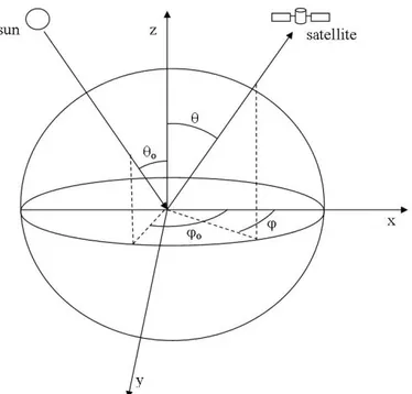
1.2.1 Geometry ConsiderationsBefore discussing remote-sensing retrieval methods in the following sections, and in subsequent chapters, it is helpful to define the frame of reference for passive remote sensing observations (in which the sun is the source of radiation). This document will use a terrestrial frame of reference, in which the sun and sensor positions are defined relative to an axis which is normal to the earth’s surface. A depiction of this frame of reference is
displayed in Figure 1.3, where θ and θo are the sensor and solar zenith angle, respectively, and φ and φo are the sensor and solar azimuth angle.
Figure 1.3: Depiction of the terrestrial frame of reference for satellite and solar positions.
A zenith angle of zero corresponds to the position which is directly overhead (also referred to as the nadir direction), a zenith angle of 90º corresponds to the direction along the horizon. The azimuth angle refers to the compass position of the sun or the sensor. The relative azimuth angle is defined relative to the forward scattering direction of the radiation, and is defined as:
) 180
( − −
=
ϕ
ϕ
ϕ
rel o (1.11)Thus, when the sun and sensor have the same azimuth angle, the relative azimuth is 180º; when they are at opposite azimuth angles, their relative azimuth is 0º. The scattering angle that corresponds to a given sun-sensor geometry is calculated from the sun and sensor zenith angles and the relative azimuth angle as follows:
rel o
o θ θ θ ϕ
θ cos sin sin cos cos
Orbiting satellite-based instruments with a fixed viewing geometry can only sample one scattering angle at a time; many are designed to scan along or perpendicular to their orbit track in order to make measurements at a larger range of scattering angles. Because satellite-based instruments are measuring light scattered from the sun, their observations generally occur at backscattering angles (Θ > 90º).
1.2.2 Satellite-Based Retrievals
While there have been several studies that propose a combination of
measurements from multiple satellite sensors (e.g. Hu et al., 2007; Satheesh et al., 2009; Vermote et al., 2007) for real-time aerosol absorption monitoring from space, there are currently only a few existing single-sensor satellite retrieval algorithms that provide regular monitoring of aerosol absorption over land. Two examples will be discussed here.
1.2.2.1 TOMS AI
The Total Ozone Mapping Spectrometer (TOMS), an ultra-violet (UV) monitoring instrument that was mounted on three different polar-orbiting satellites, provided the first global information about the location and relative abundance of UV-absorbing aerosols in the atmosphere (Herman et al., 1997; Hsu et al., 1996). The TOMS Aerosol Index (AI) is a unitless measure of aerosol absorption, calculated as
− − = calc meas I I I I AI 380 340 380 340 10 log 100 (1.13)
where I340 and I380 refer to the backscattered radiances at wavelengths of 340 and 380 nm,
respectively. The ratio of the radiances measured at these two wavelengths is compared to a calculated ratio assuming a purely gaseous atmosphere. Negative values of AI
correspond to non-absorbing aerosols; positive values correspond to aerosols that absorb in the UV, a large component of which is dust and biomass burning emissions. While the AI is not in itself a measure of the absorbing efficiency of particles, attempts have been made to use the information to retrieve the aerosol complex index of refraction in the UV (e.g. Colarco et al., 2002). It should be noted, however, that the AI is sensitive to the height of the aerosol plume (Torres et al., 1998), which will affect the retrieval uncertainty.
1.2.2.2 DeepBlue
One method currently being applied to passive satellite measurements for
absorption retrievals over land is the DeepBlue algorithm (Hsu et al., 2004; , 2006). The algorithm was designed specifically to tackle the problem of retrieving aerosol properties over bright desert surfaces by making use of the fact that desert surfaces are much darker in the blue channels (412 and 490 nm) than they are in the red. The operational retrieval algorithm for the Moderate Resolution Imaging Spectroradiometer (MODIS, see Chapter 2 for a full description) employs a dark-target approach (Kaufman et al., 1997) that relies on the reflectance at 2.1 µm to be less than 0.25 (Remer et al., 2005). Over desert, the surface reflectance exceeds this value, and thus the contribution of the surface cannot be isolated from the reflectance of the earth-atmosphere system.
The DeepBlue algorithm uses a database of land surface reflectivity to construct look-up tables of the TOA reflectance ratio between the blue and red channels as a function of AOD and SSA. An example of the look-up table at 490 nm for dust aerosol is shown in Figure 1.4. The optical properties of the aerosol are assumed in the red channel,
and retrieved in the blue channels. Results from the retrieval have produced AODs that are generally within 20% of ground-based measurements.
Figure 1.4: Simulated TOA reflectance for various AODs and SSAs at 490 nm versus 670 nm for dust aerosol. Reflectance data from SeaWiFs is shown by the filled circles. From Hsu et al. (2004).
1.2.3 Ground-Based Retrievals
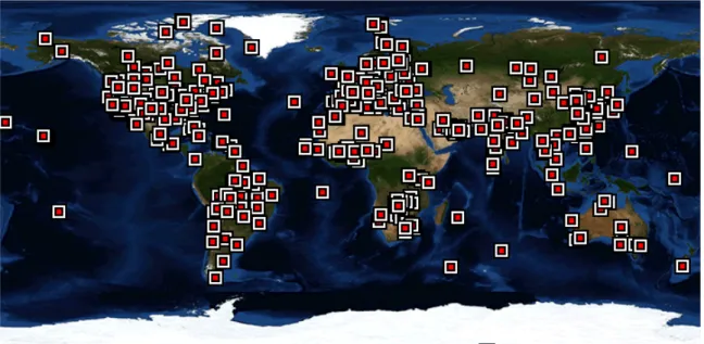
The Aerosol Robotic Network (AERONET, Holben et al., 1998) is a global network of automated sunphotometers dedicated to aerosol monitoring and
characterization at high temporal resolution and multiple spectral bands. Locations of the AERONET stations are shown in the map in Figure 1.5. The AERONET sunphotometers can sample a fuller range of scattering angles than satellite-based instruments (when the sun is at a lower elevation), given that they scan the sky throughout the day. Almucantar measurements scan the sky at the elevation of the sun, whereas principle plane
measurements scan the sky in the plane of the sun. Direct sun measurements of spectral AOD are also made. An inversion combines these measurements to retrieve the columnar aerosol size distribution, refractive index, and SSA (Dubovik and King, 2000; Dubovik et al., 2002). Accuracy of the retrievals of these properties is found to improve with a larger
coverage of scattering angles of 100º or larger (Dubovik et al., 2000), and when the aerosol loading is higher (AOD > ~0.4 at 0.44 µm).
Figure 1.5: Locations of past and existing AERONET stations. From http://aeronet.gsfc.nasa.gov.
1.3 Overview of Aerosol Impacts in North Africa
1.3.1 Aerosol Types and SeasonalityMuch of our understanding about aerosol sources and transport in North Africa has come from remote sensing observations. The largest component of the aerosol mass in North Africa is dust aerosol, which originates from the region’s numerous dust sources. TOMS AI data suggest that the majority of airborne dust in North Africa (and the world) originates in topographical lows, where alluvial flows are collected from wadi beds and salt playas (Prospero et al., 2002). Nearly all of the active dust sources in North Africa are located north of 15º N, where annual rainfall is less than 200 mm yr-1 (Figure 1.6). The single largest source in the region is the Bodele depression in Chad, as indicated by the near-persistent frequency of TOMS AI values exceeding 1.0 (Figure 1.6, region near 15º N, 15º E), and by visibility data from a nearby meteorological station which
show significant visibility reduction throughout the year, with some decreased frequency in the fall months (Mbourou et al., 1997).
Figure 1.6: Map of dust sources and elevation (shaded colors) in the global dust belt. Contours are the mean values of frequency of days per month with TOMS AI > 1.0. From Prospero et al. (2002).
The seasonality and interannual variability of dust emissions from North African sources is demonstrated in Figure 1.7. Dust activity begins at low latitudes in the winter months, when strong surface winds activate production in the Bodele depression
(Washington and Todd, 2005; Washington et al., 2006). This dust is transported across the Atlantic to South America (Prospero et al., 1981), serving as an important source of nutrients for the Amazon basin (Koren et al., 2006). Dust activity shifts northward, and also exhibits the largest spatial extent, in the spring and summer months. Strong surface heating results in rapid convective mixing that activates additional sources in western North Africa. As summer daytime boundary layers in this region extend to 600 millibars on average (Parker et al., 2005), dust is easily lofted to heights of 3-5 km, where it is transported across the Atlantic to North America (e.g. Perry et al., 1997).
Figure 1.7: Seasonal variability in 1981 (left) and interannual variability from 1982-1987 (right) of dust sources as indicated by frequency of days per month with TOMS AI > 1.0. From Prospero et al. (2002).
The onset of peak activity in dust aerosol emissions from the Bodele depression in winter coincides with the peak season of the other dominant aerosol source in North Africa: biomass burning in the Sahel. During this dry season, human-induced agricultural burning activities are widespread south of 11º N. Using satellite measurements of active
fire counts, Giglio et al. (2006) find that the peak months of fire activity in the Sahelian region are November to February (Figure 1.8). They also find that the maximum density of fires occurs in equatorial Africa with very little inter-annual variability.
Figure 1.8: Corrected fire pixel density (a) and peak month of fire activity (b) derived from Terra MODIS observations from 2000-2005. From Giglio et al. (2006).
As the dust emissions from Bodele and other regional sources are carried southward by cool, dry northwesterly winds, they intersect the biomass burning emissions, which are moving slowly northward in a region of convective instability (Haywood et al., 2008). The biomass burning emissions are pushed upward by the dust “front”, rising to higher and higher altitudes as they move further north (Figure 1.9,
Haywood et al., 2008). Some of this dust is also transported westward over the Atlantic; the plume of absorbing aerosol in January in Figure 1.7 is likely biomass-burning dominated.
Figure 1.9: Schematic cross section of the intersection between southward transported dust and northward transported biomass burning during the winter dry season in the Sahel. From Haywood et al. (2008).
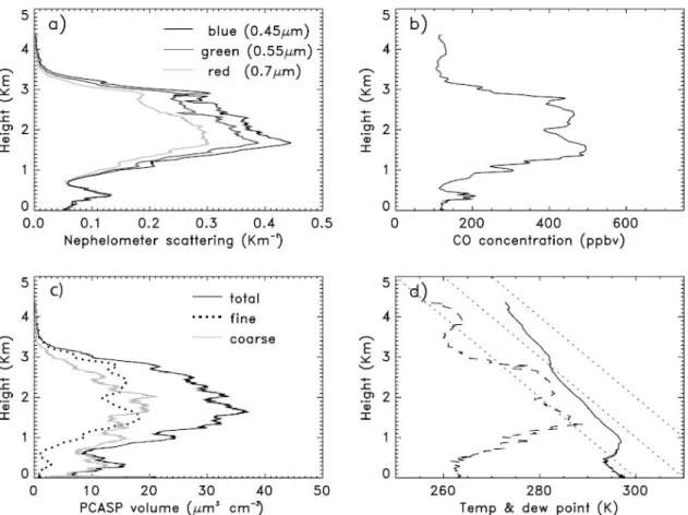
During the Dust and Biomass-burning Aerosol Experiment (DABEX) campaign, which was a component of the African Monsoon Multidisplinary Analysis (AMMA) study, research flights were performed through aerosol plumes during January and February 2006 near Niamey, Niger. Although there was significant variability in individual profiles of aerosol measured during the campaign, they typically included an elevated layer of biomass burning aerosol, with dust dominating the boundary layer (Johnson et al., 2008a). An example from 19 January 2006 is shown in Figure 1.10. The dominance of dust aerosol below 1 km is indicated by the near-zero spectral dependence of aerosol scattering, and the fact that the aerosol volume concentration is primarily made up of coarse mode particles. Above this layer, the spectrally-dependent aerosol scattering and increased fine mode particle concentration indicate the presence of biomass burning
aerosol; however, since coarse mode concentrations are similar to those in the boundary layer, the biomass burning aerosol has mixed with dust. Indications of aging of biomass burning aerosol are also present, which does result in a larger mean size of the aerosol. A mid-level inversion, which is a common feature of the seasonal circulation pattern in this region (Figure 1.9) keeps the aerosol confined below 4 km.
Figure 1.10: Vertical profiles of nephelometer scattering (a), CO concentration (b), aerosol volume concentration (c), and temperature and dew point (d) determined from in situ aircraft measurements near
Niamey, Niger on 19 January 2006. From Johnson et al. (2008a).
1.3.2 Physical and Optical Properties
Several field campaigns and lab studies have been performed in an effort to characterize the optical properties of dust and biomass burning aerosol originating from North Africa (e.g. Haywood et al., 2008; Tanré et al., 2003; Volz, 1973). A few key results will be described here.
As mentioned above with respect to vertical profiles of aerosol, the majority of biomass burning aerosol mass is located in the fine mode (Dp <1 µm), whereas the majority of dust aerosol mass is located in the supermicron coarse mode. Johnson et al (2008a) find that the particle volume measured in biomass burning aerosol plumes during DABEX was dominated by particles smaller than 0.35 µm in diameter. The size
distribution of both aerosol types can change as their atmospheric residence time
increases. As biomass burning particles age, they increase in size due to coagulation and condensation, and may also grow by water uptake (Carrico et al., 2010). As dust plumes are transported away from sources, larger particles are lost due to gravitational settling, although Maring et al. (2003) find that dust size distributions exhibit little change in the contribution of particles with diameters smaller than ~7 µm, even in cases of trans-Atlantic transport.
Both dust and biomass burning aerosol optical properties are dependent on their source, age, and size. Although many studies confirm that fine mode dust aerosol is almost non-absorbing in the visible (SSA ~ 0.99 at 0.55 µm), McConnell et al. (2008) find that including the coarse mode from their dust measurements resulted in a SSA that was closer to 0.9. Furthermore, dust absorption is dependent on the mineral composition (e.g. Sokolik and Toon, 1999) and there is some evidence that dust from certain source regions is more absorbing than others. Formenti et al. (2008) find that dust from sources near the Sahel and in Mauritania has a higher content of iron oxides such as hematite, which is absorbing in shorter wavelengths, than dust from the Bodele depression. Alfaro et al. (2004) find similar evidence that dust collected in Niger is more absorbing than dust from the northern Sahara. Results using the DeepBlue algorithm (Hsu et al., 2004) also
suggest that Bodele dust may be less absorbing in the blue channels than dust from other sources (Figure 1.11). Over the Saharan desert, these variations in absorption could lead to changes in the sign and/or magnitude of the TOA forcing.
Figure 1.11: DeepBlue retrievals of SSA at 412 and 490 nm (value at 670 is assumed to be 1.0) downwind of Bodele and an Algeria/Niger dust source. From Hsu et al. (2004).
The absorptivity of biomass burning aerosol depends on the fraction of elemental carbon and organic species that are present in the aerosol, which varies with fuel type and fire conditions (McMeeking et al., 2009; Reid and Hobbs, 1998). The results of Johnson et al. (Johnson et al., 2008a) indicate that fresh biomass burning emissions in North Africa are more absorbing than those measured in southern African during the SAFARI-2000 campaign (Haywood et al., 2008), which could be due to differences in fuel type between the two regions.
1.4 Critical Reflectance Principle
The previous sections have shown that aerosol absorption over North Africa can be highly variable in space and time, and accurate knowledge of aerosol absorption properties is critical for understanding the impact of aerosols on climate in desert regions, and for tracking their emission and transport patterns. Because of the highly-reflective surface, the sign of the TOA aerosol forcing is quite sensitive to SSA. But, without reliable information about the underlying properties of the desert surface, one cannot determine the critical SSA at which the transition from TOA cooling to TOA warming occurs. The aerosol critical reflectance (Fraser and Kaufman, 1985; Kaufman, 1987), however, is a parameter that can be determined without knowledge of the surface reflectance and is uniquely related to the SSA for aerosol of a fixed size and scattering phase function. It can also be used to determine the relationship between the observed SSA and the critical SSA, and can thus provide some information about the sign of the TOA aerosol forcing, as well as its spectral dependence.
1.4.1 Definition and Assumptions
The critical reflectance principle was introduced by Fraser and Kaufman (1985) and further developed by Kaufman (1987) as an intrinsic property of aerosol that could provide information about the absorption properties of aerosol. It states that, for a given aerosol of fixed SSA and phase function, there is a certain surface reflectance, ρc, at
which a change in aerosol loading does not affect the reflectance of the earth-atmosphere system. If a more-absorbing aerosol is added over the critical surface reflectance, or if the aerosol is moved over a surface with a reflectance that is greater than ρc, the aerosol will
is added, or if the aerosol is moved over a surface with a reflectance less than ρc. Because
the critical surface reflectance is relatively independent of AOD, its determination does not require information about the aerosol loading.
The demonstration of the critical reflectance concept is shown in Figure 1.12, using radiative transfer calculations with an assumed aerosol size distribution and
refractive index at a wavelength of 0.61 µm. The difference between the TOA reflectance and the surface reflectance (y-axis) is plotted as a function of the surface reflectance for AODs of 0, 0.2, 0.4, and 0.6 for an SSA of 0.96 and 0.81 (assuming a fixed scattering phase function for both). For each SSA there is a surface reflectance at which the TOA reflectance is not sensitive to changes in AOD. Physically, this point represents a balance between increased aerosol backscatter at TOA and increased absorption of the surface contribution as the aerosol loading increases. This balance occurs at a lower critical reflectance for the more absorbing SSA, and will also change as a function of the solar zenith angle, satellite view angle, and relative azimuth, all of which were held constant in the calculations shown in Figure 1.12.
Provided the underlying surface has some variability over which to see changes in the TOA reflectance across an image, the critical reflectance can be used to derive SSA from satellite images of the same scene with different aerosol loadings but the same solar and viewing geometries. The assumptions required to apply the critical reflectance principle to derive SSA from satellite images are (Kaufman, 1987):
1. The aerosol optical depth is constant over the area contained by the pixel 2. The surface reflectance is invariant between the two comparison days
3. The surface is Lambertian, or, its angular variability in reflectance does not affect the TOA reflectance between the two comparison days
4. The phase function of the “background” aerosol and gaseous composition is similar between the two days
Figure 1.12: The difference between the TOA upward reflectance and the surface reflectance, ρ, as a function of ρ for AOD = 0, 0.2, 0.4 and 0.6 and two different SSAs, 0.81 and 0.96. From Kaufman (1987).
1.4.2 Foundational Work and Applications 1.4.2.1 Demonstration of Principle
Fraser and Kaufman (1985) demonstrated the use of the critical reflectance principle on satellite imagery by plotting the reflectance measured by the Landsat instrument on a polluted day over Washington, D.C. against reflectances measured on a cleaner day over the same area (Figure 1.13). From this figure, the critical reflectance was determined to be 0.18. Kaufman (1987) ascribes the scatter in the data to various effects:
1. Variation in the surface reflectance between the two days
2. Different background aerosol composition between the two days 3. Changing atmospheric characteristics between the two days 4. Differences in the registration between the two images 5. Adjacency effects due to atmospheric scattering
6. Difference in surface reflectivity between the two days that is due to small variations in the solar zenith angle and satellite view angle and a non-Lambertian surface
Figure 1.13: Scatter diagram of Landsat reflectances measured on a polluted day compared to reflectances measured on a clean day over Washington, D.C. From Kaufman (1987).
1.4.2.2 Saharan Dust Absorption
Kaufman et al. (2001) used the critical reflectance principle to demonstrate that the absorption of Saharan dust aerosol was much smaller than currently accepted values, or those being used in global models to estimate aerosol effects (e.g. Sokolik and Toon,
1999; Sokolik et al., 1998). The World Meteorological Organization suggested that the imaginary index of refraction, k, for Saharan dust was 0.008 at a wavelength of 0.5 µm (WMO, 1983) corresponding to a SSA of 0.63. Kaufman et al. (2001) compared a Landsat image of a major dust event to a cleaner image to show that the dust
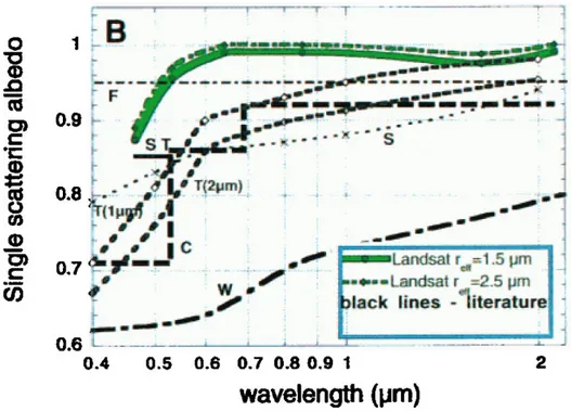
systematically increased the spectral reflectance at nadir view across the Western Sahara. Using the critical reflectance technique, they derived a SSA of 0.97 ± 0.02 at 0.64 µm, with a more absorbing SSA at 0.47 µm (<0.9) and near-zero absorption in the near-IR channels. Results of the case study are shown in Figure 1.14.
Figure 1.14: Spectral SSA for a Saharan dust event retrieved from Landsat measurements (green lines) compared to other estimates from the literature (black lines). From Kaufman et al. (2001).
1.4.3 Other Applications of the Principle
Since the application of the principle for the Saharan dust case in 2001, critical reflectance has been used to derive aerosol optical properties, but mainly in instances where temporally- and spatially-averaged SSA is sought. Two such studies that have been reported in the peer-reviewed literature are described here.
1.4.3.1 Average Saharan Dust Absorption
Yoshida and Murakami (2008) used the critical reflectance in order to determine average dust aerosol properties in the entire Sahara region. They used four years of data from the MODIS instrument to derive average reflectances during clean conditions and dusty conditions respectively. They compared the difference between these reflectances to find the TOA reflectance on the clean day that corresponded to a zero change in the TOA reflectance between the two days. They defined this as the critical reflectance at TOA, and used average AOD values from AERONET to derive a corresponding SSA. They retrieved an average SSA of 0.936 at 0.466 µm, and 0.976 at 0.553 µm. Their resulting SSAs (Figure 1.15) agree quite well with the estimates from Kaufman et al. (2001), although Yoshida and Murakami (2008) found the dust to be less absorbing at 0.466 µm.
Figure 1.15: Average spectral SSA for Saharan dust retrieved from MODIS measurements, compared to other estimates from the literature. From Yoshida and Murakami (2008).
1.4.3.2 Aerosol Properties over Saudi Arabia
Satheesh and Srinivasan (2005) extended the critical reflectance principle to an application that does not require assumptions about aerosol properties. They compared satellite measurements of TOA albedo change and ground-based measurements of AOD at the Solar Village AERONET station in Saudi Arabia to derive a critical aerosol optical depth that results to a zero change in the TOA albedo during November and July 2000 (Figure 1.16, shown for November), the two months corresponding to periods of high and low absorption at the site, respectively. Assuming that the bulk aerosol properties were unchanged over the course of the month, they derived an SSA of 0.89 and 0.97 for the two months at a wavelength of 0.5 µm. These estimates agreed well with SSA-critical AOD relationships simulated with a radiative transfer model.
Figure 1.16: Change in TOA albedo measured by satellite as a function of AOD measured by AERONET at Solar Village, Saudi Arabia. From Satheesh and Srinivasan (2005).
1.5 Objectives
Although previous applications of the critical reflectance method have produced SSA estimates that are in agreement with estimates from other retrieval techniques, they do not demonstrate the feasibility of using the principle for real-time aerosol absorption
monitoring at finer spatial resolution over desert surfaces. Kaufman (1987) outlined some of the limitations and sources of uncertainty in applying the critical reflectance to
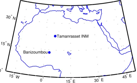
estimate SSA, but a full assessment of the utility of critical reflectance retrievals over desert, and over North Africa in particular, has not been reported to date. This work investigates the sensitivity of the critical reflectance parameter to assumed aerosol physical and optical properties, as well as solar and viewing geometries that are representative of satellite-based observations, using the SBDART radiative transfer model and a T-matrix code. We use our findings to build look-up-tables which we apply to retrieve spectral SSA from critical reflectance, derived from MODerate resolution Imaging Spectroradiometer (MODIS) Level 1B data, in the vicinity of two North African AERONET sites: Tamanrasset, a site in the Algerian Sahara, and Banizoumbou, a site in Niger. We evaluate our results with comparisons to the AERONET-retrieved SSA and size distributions, DeepBlue SSA, as well as measurements of TOA and surface fluxes from the RADAGAST experiment (Slingo et al., 2009) and TOA albedo from CERES. Our results reveal the main sources of uncertainty in the spectral SSA derived over North Africa from the critical reflectance, and help us to define the conditions in which the retrieval will be best applied in this region. Implications of the SSA uncertainties for the ability to estimate TOA aerosol forcing over the AERONET sites are also explored.
2 Retrieval Method and Sensitivity
2.1 Observations
2.1.1 The MODIS Instrument
The Moderate Resolution Imaging Spectroradiometer (MODIS) is a passive radiometer aboard NASA’s Terra and Aqua satellites, with 36 spectral channels ranging from 0.41 µm to 15 µm. Both satellites follow a sun-synchronous near-polar orbit, with the Terra-MODIS instrument crossing the equator at roughly 10:30 a.m. local time, and the Aqua-MODIS instrument crossing the equator at roughly 1:30 p.m. local time. MODIS achieves global coverage approximately every two days, with repeat orbits occurring every 16 days. The Aqua-MODIS instrument is part of the A-train, a
constellation of satellites in which both active and passive sensors observe the same spot on earth within a few minutes of each other during local afternoon time. One of the reasons for these near-simultaneous measurements is to better quantify the anthropogenic aerosol effect at the top of the atmosphere (Anderson et al., 2005).
The seven channels that are used in the MODIS operational aerosol retrieval algorithm over ocean (Remer et al., 2005) are Bands 1 – 7, which span the spectral range from 0.459 – 2.155 µm. The bandwidths, weighted central wavelengths, and spatial resolutions of these channels are listed in Table 2.1. The weighted central wavelengths were determined by integration of the channel-averaged response function of the MODIS instrument (Remer et al., 2006).
Table 2.1: Bandwidth, central wavelength and spatial resolution of MODIS Bands 1 – 7.
Band Bandwidth (µm) Weighted central wavelength (µm) Spatial resolution at nadir (m) 1 0.620 – 0.670 0.646 250 2 0.841 – 0.876 0.855 250 3 0.459 – 0.479 0.466 500 4 0.545 – 0.565 0.553 500 5 1.230 – 1.250 1.243 500 6 1.628 – 1.652 1.632 500 7 2.105 – 2.155 2.119 500
2.1.2 Processing MODIS Level 1B Data
The analysis used in this study begins with MODIS Level 1B data, obtained from LAADS (Level 1 and Atmosphere Archive and Distribution System) Web
(http://ladsweb.nascom.nasa.gov/). Because the critical reflectance must be derived by comparing images with the same solar and viewing geometry, we obtain data for pairs of images with different aerosol loading that are 16 days apart. The Level 1B files contain geolocated reflectance factors at the 36 MODIS bands; we use only the seven bands used in the operational MODIS algorithm, along with one additional band (1.38 µm) for cloud screening purposes. The reflectance is a unitless quantity that is simply the outgoing radiance at TOA normalized by the incoming solar irradiance, which has also been corrected for solar zenith angle variation. The reflectance, ρλ, is defined as
) cos( , o o F L θ π ρ λ λ λ = (2.1)
where Lλ is the measured radiance (in W m-2 ster-1), Fo,λ is the solar irradiance (in W m-2),
and θo is the solar zenith angle. The reflectance factor given in the MODIS Level 1B data
is simply the product of ρλ and cos(θo), therefore we normalize the data by cos(θo) to
2.1.2.1 Correction for Gaseous Absorption and Clouds
To isolate the component of the reflectance that is due to aerosol scattering, we correct the reflectance data for absorption due to water vapor, ozone, and carbon dioxide, and for the presence of clouds within the image. The gaseous absorption correction is the same as that used in the operational MODIS aerosol retrieval algorithm (Remer et al., 2006), and requires ancillary data on trace gas concentrations. Column precipitable water data from 1o x 1o NCEP reanalysis (obtained from http://www.esrl.noaa.gov/psd/ data/ reanalysis/reanalysis.shtml) are used for the water vapor correction; the ozone correction is done using the 1o x 1o TOAST (Total Ozone Analysis using SBUV/2 and TOVS) column ozone product (obtained from http://www.osdpd.noaa.gov/ml/air/ toast.html). We assume climatological values of optical depth for the carbon dioxide correction.
We calculate transmission factors, Tλ, for each gas from the ancillary gas
concentration data. For water vapor:
)) )) (ln( ) ln( exp(exp( 1,2 2,2 3,2 2 2 K K Gw K Gw TλHO = HλO+ HλO + HλO (2.2) For ozone: ) exp( 3 3 GK D TλO = λO (2.3)
For carbon dioxide:
) exp( 2 2 CO CO G Tλ = τλ (2.4)
where w is the column precipitable water vapor (in centimeters), D is the column ozone (in Dobson units), Kλ is the absorption coefficient for water vapor or ozone, and τλCO2 is
the climatological optical depth of carbon dioxide. The absorption coefficients and climatological optical depth values used in the correction can be found in Table 2.2. G is
the air mass factor, which is calculated from the solar (θo) and sensor (θ) zenith angles as follows: ) cos( 1 ) cos( 1 θ θ + = o G (2.5)
The corrected reflectance, ρaer,λ,is calculated from the MODIS Level 1B reflectance by
λ λ
λ
ρ
ρ
gasaer, =T (2.6)
where Tλgas is the total gas transmission factor, which is simply the product of the individual gas transmission factors for water vapor, ozone, and carbon dioxide:
2 3 2O O CO H gas T T T Tλ = λ λ λ (2.7)
Table 2.2: Gas absorption coefficients for water vapor and ozone, and climatological optical depth values of carbon dioxide. Wavelength (µm) HO K 2 , 1λ O H K 2 , 2λ O H K 2 , 3λ 3 O Kλ CO2 λ τ 0.466 4.26 x 10⁻⁶ 0.553 1.05 x 10⁻⁴ 0.646 -5.73888 0.925534 1.543 x 10⁻² 5.09 x 10⁻⁵ 0.855 -5.32960 0.824260 1.947 x 10⁻² 1.243 -6.39296 0.942186 1.184 x 10⁻² 4.196 x 10⁻⁴ 1.632 -7.76288 0.979707 9.367 x 10⁻³ 8.260 x 10⁻³ 2.119 -4.05388 0.872951 5.705 x 10⁻² 2.164 x 10⁻²
We perform cloud screening on the reflectance data using the same technique as described by Martins et al. (2002) for the MODIS over-ocean cloud screening algorithm, which we have modified to be applicable over land. It consists of a combined test using the spatial homogeneity of the reflectance along with absolute reflectance thresholds. We use 0.466 µm to identify low clouds, and Band 26 (1.38 µm) to identify high clouds. Figure 2.1 demonstrates that the reflectance associated with aerosol plumes (shown at 0.553 µm, a channel we do not use for our cloud screening) tends to be much more spatially-homogeneous than that associated with clouds, although there is a relatively broad transition region between the two. Martins et al (2002) estimate that their chosen
threshold allows for 1 – 5% cloud contamination of the pixels. Our algorithm constructs a 3 x 3 pixel mask that is flagged as cloud if the standard deviation of the reflectance of the 3 x 3 pixels is greater than 0.01 at 0.466 µm or 0.007 at 1.38 µm. It is also flagged as cloud if the gas-corrected reflectance in either of these bands exceeds a maximum threshold value (0.4 at 0.466 µm and 0.1 at 1.38 µm). The effectiveness of these thresholds over land has not been rigorously tested, however, so it is possible that our algorithm allows for a higher fraction of cloud contamination than the over-ocean algorithm.
Figure 2.1: Histogram of 3 x 3 pixel reflectance standard deviation for 0.553 µm, demonstrating the separation between aerosol and cloud. The “operational thresh” line refers to the threshold used in the
operational over-ocean MODIS aerosol retrieval algorithm. From Martins et al. (2002). 2.1.2.2 Remapping
Next, in order to facilitate pixel-to-pixel comparison of two images, we remap the reflectance data onto an equal latitude-longitude grid. Even though this analysis makes use of the MODIS 16-day repeat viewing cycle to compare images with the same geometry, the two images will not be identical. Small orbital shifts cause slight changes
in viewing and solar zenith angle for a given pixel relative to 16 days prior. Also, because MODIS has a relatively large footprint, the images it produces are not on a regular grid. The instrument samples by scanning from left to right over the curved surface of the earth, resulting in an increased pixel size as the sensor moves away from nadir. This is known as the “bowtie effect”, where consecutive scans partially overlap at non-nadir angles (Figure 2.2) resulting in over-sampling of these pixels. We do not assess the effects of the overlapping sampling in our analysis, but we do consider the change in pixel size when choosing our remapping grid. The pixels at the edge of a MODIS image are about three times the length and width of those at nadir, so, in order to not perform subpixel interpolation in our remapping process, we aggregate the reflectances up to a grid of about 1.5 km. This is done at all seven channels, despite the fact that Channels 1 and 2 have a resolution of 250 meters.
Figure 2.2: Representation of three consecutive MODIS scans consisting of 10 pixels along the flight direction, and 22 along the scan direction. From eoweb.dlr.de.
2.1.2.3 Data Fitting and Assumptions
Once the data are remapped to the same grid, the area of a larger pixel upon which to retrieve a constant SSA is defined. The area must be large enough to contain some variability in surface reflectance, so that there is some dynamic range of clean day
reflectances over which to perform a data regression. But, the pixel must not be too large as to contain significant spatial variations in aerosol loading. We choose an area of 10 by 10 pixels (approximately 15 by 15 km). Within each box, which we will call the retrieval pixel, the remapped reflectance data are matched in space, and the reflectances on the polluted day are regressed against the reflectances of the cleaner day. The slope and intercept are determined using a robust linear fitting procedure, in order to give less weight to data outliers. An example scatter plot containing a few outlying reflectance points is show in Figure 2.3. The point at which the fit line crosses the one-to-one line is the critical reflectance at TOA. The y-intercept will be referred to as the path radiance, which is proportional to the optical depth difference between the clean and the polluted day. If there are any missing data within the retrieval pixel due to cloud screening, no retrieval is performed within the box.
0 0.2 0.4 0.6 0.8 1 0 0.1 0.2 0.3 0.4 0.5 0.6 0.7 0.8 0.9 1 Clean refl Polluted refl
Figure 2.3: Example of a scatter plot of polluted versus clean reflectances for one 10 x 10 pixel box. The black line is the one-to-one line; the red line is the linear fit determined using the robust regression routine.
2.1.2.4 Post Processing and Error Estimation
There are a few diagnostic tests that we use to determine if a retrieval pixel should be eliminated a posteriori. First, in order to ensure that the slope of the fit line is not so similar to the one-to-one line that it inhibits the precise determination of the critical reflectance, and to prevent the inclusion of pixels in which the cleaner day is actually more polluted than the polluted day (resulting in negative path radiance), we arbitrarily ascribe a minimum path radiance threshold of 0.02. Secondly, if the robust fit results in a negative critical reflectance, or a critical reflectance that exceeds 1.0, that pixel is also discarded.
Because the uncertainty in the measured reflectances from MODIS is only on the order of ± 2% (Remer et al., 2005), we assume that the uncertainty in the critical
reflectance is a combination of the uncertainties associated with the data fitting routine and the assumptions listed in Section 1.4.1. We will address the former uncertainty source here, and the latter sources using sensitivity tests in subsequent chapters. We consider one measurement of the uncertainty due to data fitting to be the standard deviation of the residuals of the fit line:
1 ) ( 1 2 , − − =
∑
= N y y N i i fit i residσ
(2.8)where yi the TOA reflectance value of a single pixel on the polluted day, and yfit,i is the
y-value of the linear fit to the TOA reflectance data. In order to consider the number of outliers in the determination of which pixels to keep from the retrieval, we also throw out those in which more than 10 pixels have a residual reflectance greater than 2σresid.
A second measure of the fitting uncertainty is determined through error propagation. Given that we perform a linear fit to the reflectance data, the critical reflectance, Rcrit, is simply
m b Rcrit − = 1 (2.9)
where m is the slope of the linear fit and b is the y-intercept. Given the general error propagation equation 2 2 2 2 z z y x x S z x S y x S ∂ ∂ + ∂ ∂ = (2.10)
the error in the critical reflectance is
2 2 2 2 1 1 1 m b Rcrit m b m σ σ σ − + − = (2.11)
where σb is the uncertainty in the y-intercept as determined from the robust fitting routine
and σm is the uncertainty in the slope of the linear fit.
2.2 Forward Model
We use a standard, publicly-available radiative transfer model, SBDART, to build a look-up table (LUT) of critical reflectance as a function of SSA for different assumed aerosol size distributions and refractive indices, as well as a range of solar and viewing geometries that are applicable to the MODIS instrument orbit and scanning
characteristics. This section details the radiative transfer model set-up, aerosol model assumptions and phase function calculations, and the LUT-building procedure. LUT results and their implications for the critical reflectance sensitivity to aerosol physical and optical properties, as well as the model set-up, will be included in Section 2.3.
2.2.1 Radiative Transfer Model Set-Up
The Santa Barbara DISORT Atmospheric Radiative Transfer (SBDART) model (Ricchiazzi et al., 1998) is a multi-stream radiative transfer model that uses DISORT (Discrete Ordinate Radiative Transfer, Stamnes et al., 1988) to integrate the radiative transfer equation for a plane-parallel vertically-inhomogeneous atmosphere. We use the most recent version of the code, version 2.4 (obtained from ftp://ftp.icess.ucsb.edu/pub/ esrg/sbdart/). The model can handle a maximum of 40 streams, but we use the default 20 streams because the simulations can be performed 10 times faster in this mode. A
discussion of the impact of the number of streams used in SBDART can be found in Section 2.5.4.
The model set-up we use ascribes 32 layers to the atmosphere: 25 equidistant layers between 0 and 25 km, 5 equidistant layers between 25 and 50 km, and 2
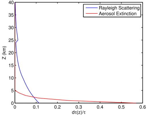
equidistant layers between 50 and 100 km. Gaseous concentrations are assumed based on the standard subarctic summer atmosphere contained in the SBDART database. Because we correct the MODIS data for gaseous absorption, we set column ozone, water vapor, and carbon dioxide concentrations to zero in the model. We also ascribe the average surface elevation of each region of interest (given in Chapter 3 for the case study sites), so as to scale the Rayleigh scattering accordingly. We apportion the total aerosol optical depth into the lowest 5 km of the atmosphere. This height was chosen based on average vertical profiles of aerosol extinction measured in the Sahel region during the Dust and Biomass Burning Experiment (DABEX) campaign (Figure 2.4, Johnson et al., 2008b). The assumed vertical distribution of the fractional optical depth (dτ(z)/ τ) of each layer is
shown in Figure 2.5, for both aerosol extinction and Rayleigh scattering (at 0.466 µm). Below the atmosphere, isotropic scattering from the surface is assumed.
Figure 2.4: Average vertical profiles of aerosol extinction from the DABEX campaign for (a) total aerosol and (b) biomass burning and dust components, separately. From Johnson et al. (2008b).
0 0.1 0.2 0.3 0.4 0.5 0.6 0 5 10 15 20 25 30 35 40 Z (km) dτ(z)/τ Rayleigh Scattering Aerosol Extinction
Figure 2.5: Vertical profile of the fractional optical depth assumed for Rayleigh scattering (blue) at 0.466 µm and aerosol extinction (red) at all wavelengths in SBDART.
Aerosol single-scattering albedo, optical depth, and scattering phase function are input into SBDART for each layer below 5 km. Expansions of the scattering phase
function are performed in the model using Legendre polynomials of the order N. The expansion takes the form
∑
− = N l l lP P 0 ) ( ) (µ χ µ (2.12)where µ is the cosine of the scattering angle, Pl is the lth order Legendre polynomial and
χl are the lth order expansion coefficients
∫
− + = 1 1 ( ) ( ) 2 ) 1 2 ( µ µ µ χl l P Pl d (2.13)The phase function inputs required by SBDART are the Legendre moments of the phase function, Ml, given as
∫
∫
− − = 1 1 1 1 ) ( ) ( ) ( µ µ µ µ µ d P d P P Ml l (2.14)We use polynomials with 128 terms in our simulations, in order to sufficiently represent more complicated Mie phase functions when spherical particles are assumed.
2.2.2 Aerosol Models and Phase Function Calculations
Because we are performing retrievals over a region that is often impacted by non-spherical dust particles, we do not use a Mie code to determine the scattering
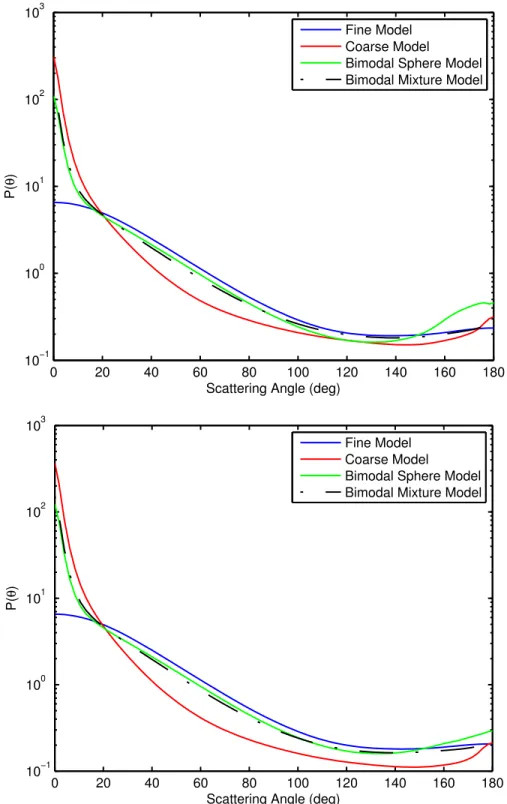
characteristics of our aerosol models. Aerosol phase functions and single-scattering albedos are instead modeled using a modified T-matrix code (Dubovik et al., 2002) for the seven MODIS channels we use in the retrieval. The code simulates a population of particles as spheres, spheroids, or a mixture of both. The user specifies the particle size distribution and the percent sphericity (as the fraction of the total particle volume made up of spherical particles) of a particle population. We use 22 size bins evenly spaced on a
log scale, ranging from 0.05 to 15 µm in radius, which is consistent with the length and range of the size distribution vector output by the standard AERONET retrieval. We assume four different aerosol models: fine mode spheres, a coarse mode made of
primarily spheroids (percent sphericity = 0.5%), bimodal spheres, and bimodal spheroids (percent sphericity = 4%). The bimodal size distribution (Figure 2.6) was taken from an AERONET retrieval over the Banizoumbou station on 19 January 2006. For the coarse model, we simply assume the coarse mode of this distribution, and the fine mode for the fine model. The value chosen for percent sphericity of the bimodal spheroid distribution is assumed based on the reported value from AERONET on 19 January 2006.
10−2 10−1 100 101 102 0 0.02 0.04 0.06 0.08 0.1 0.12 0.14 0.16 Radius (µm) dV/dlnr ( µ m 3 /µ m 2 )
Figure 2.6: Bimodal size distribution model (from Banizoumbou AERONET site on 19 January 2006).
For each wavelength and size model we assume the real refractive index to be 1.53, which is the same value assumed in the MODIS operational algorithm from 0.466 to 0.855 µm for the dust-like aerosol model (Remer et al., 2005). We vary the imaginary part of the refractive index in order to simulate a wide range of aerosol absorption values.
For each refractive index and wavelength, the code estimates the scattering phase function at 83 scattering angles, as well as the SSA of the particle population. The minimum imaginary refractive index that can be input into the T-matrix code is 0.0005, so the largest SSA we can simulate is slightly less than 1.0 (Table 2.3). For the fine and bimodal models we vary the imaginary part from 0.0005 to 0.030. For the coarse model, we vary the imaginary part from 0.0005 to 0.015. The corresponding SSAs for the maximum imaginary values assumed are listed in Table 2.4.
Table 2.3: SSAs estimated using the T-matrix code with k = 0.0005 for the four aerosol models.
Wavelength (µm)
Fine Model Coarse Model Bimodal Sphere Model Bimodal Spheroid Model 0.466 0.9973 0.9819 0.9922 0.9922 0.553 0.9970 0.9848 0.9917 0.9917 0.646 0.9966 0.9868 0.9912 0.9914 0.855 0.9955 0.9896 0.9906 0.9911 1.243 0.9920 0.9923 0.9912 0.9920 1.632 0.9860 0.9938 0.9925 0.9932 2.119 0.9741 0.9950 0.9939 0.9943
Table 2.4: SSAs estimated using the T-matrix code with k = 0.015 for the coarse aerosol model and 0.030 for the other three models.
Wavelength (µm)
Fine Model Coarse Model Bimodal Sphere Model Bimodal Spheroid Model 0.466 0.8584 0.7582 0.7978 0.8009 0.553 0.8465 0.7787 0.7796 0.7844 0.646 0.8298 0.7947 0.7609 0.7678 0.855 0.7841 0.8185 0.7324 0.7441 1.243 0.6726 0.8462 0.7208 0.7382 1.632 0.5431 0.8661 0.7372 0.7541 2.119 0.3915 0.8835 0.7633 0.7761
2.2.3 Critical Reflectance LUT Building
The computed phase functions and SSAs for each size model and refractive index are input into SBDART to simulate top-of-atmosphere radiances from which a critical reflectance can be determined. We perform our simulations at the same geometries as the MODIS operational algorithm: nine solar zenith angles (6, 12, 24, 36, 48, 54, 60, 66, and