IT 17 034
Examensarbete 15 hp
Juni 2017
Quadratic Programming Models
in Strategic Sourcing Optimization
Daniel Ahlbom
Institutionen för informationsteknologi
Teknisk- naturvetenskaplig fakultet UTH-enheten Besöksadress: Ångströmlaboratoriet Lägerhyddsvägen 1 Hus 4, Plan 0 Postadress: Box 536 751 21 Uppsala Telefon: 018 – 471 30 03 Telefax: 018 – 471 30 00 Hemsida: http://www.teknat.uu.se/student
Abstract
Quadratic Programming Models in Strategic Sourcing
Optimization
Daniel Ahlbom
Strategic sourcing allows for optimizing purchases on a large scale. Depending on the requirements of the client and the offers provided for them, finding an optimal or even a near-optimal solution can become computationally hard. Mixed integer programming (MIP), where the problem is modeled as a set of linear expressions with an objective function for which an optimal solution results in a minimum objective value, is particularly suitable for finding competitive results.
However, given the research and improvements continually being made for quadratic programming (QP), which allows for objective functions with quadratic expressions as well, comparing runtimes and objective values for finding optimal and approximate solutions is advised: for hard
problems, applying the correct methods may decrease runtimes by several orders of magnitude. In this report, comparisons between MIP and QP models used in four different problems with three different solvers
were made, measuring both optimization and approximation performance in terms of runtimes and objective values. Experiments showed that while QP holds an advantage over MIP in some cases, it is not consistently efficient enough to provide a significant improvement in comparison with, for example, using a different solver.
Tryckt av: Reprocentralen ITC IT 17 034
Examinator: Olle Gällmo Ämnesgranskare: Di Yuan
Daniel Ahlbom, Uppsala University 2017
Acknowledgements
I would like to express my deepest gratitude to the following: Professor Arne Andersson at Trade Extensions, for being my supervisor and introducing me to a project with great depth and learning opportunities; Dr. Fredrik Ygge at Trade Extensions, for being an advisor providing the guidance, discussions and problems necessary for making the project interesting; and Professor Di Yuan at Uppsala University, for providing much needed insights and taking the time and effort to criticize this report into legibility.
Contents Daniel Ahlbom, Uppsala University 2017
Contents
1 Introduction 4
2 Background 5
2.1 Computing Strategic Sourcing . . . 5
2.2 Solving Computationally Hard Problems . . . 5
2.3 Mixed Integer Linear Programming . . . 5
2.4 Quadratic Programming . . . 6
2.5 Approximation . . . 6
2.6 Modeling with AMPL . . . 6
3 Comparison of MIP and QP in Sourcing Problems 9 3.1 Seller Discounts . . . 9 3.2 Supply Restrictions . . . 11 3.3 Regional Division . . . 16 3.4 Reserved Price . . . 20 4 Summary 24 4.1 Conclusion . . . 24 4.2 Future Work . . . 24 References 25 A Prerequisite knowledge 26 A.1 NP-completeness . . . 26
A.2 Linear Algebra . . . 26
A.3 Convex Functions and Sets . . . 27
B Experiments 28 B.1 Testing platform . . . 28
B.2 Datasets . . . 28
B.3 AMPL Implementations . . . 28
Glossary Daniel Ahlbom, Uppsala University 2017
Glossary
AMPL A Mathematical Programming Language: A modeling language suitable forMixed Integer Programming
(MIP)andQuadratic Programming (QP)solving technologies. Official site as of June 27, 2017: http://ampl.com/.
Constraint Boundaries that a solution must satisfy in order to be valid..
Decision variable Variables for which the value has to be determined in order to find a solution.
Gurobi A solver suitable for MIP and QP optimization. It supports convex and non-convex problems with continuous and non-continuous variables in any combination forMIP, whileQPrequires that the problem is convex, or that any variable-by-variable multiplication to consist of a binary variable on either side. Official site as of June 27, 2017: http://www.gurobi.com/.
Knitro A solver suitable forQPoptimization using local search. It supports convex and non-convex problems with continuous and non-continuous variables in any combination. Official site as of June 27, 2017: https://www.artelys.com/en/optimization-tools/knitro.
LP Linear Programming: A solver technology where models are written using linear relations. Discussed in
2.3: Mixed Integer Linear Programming.
MiniSAT A solver suitable for Boolean Satisfiability Problem (SAT) problems. Official site as of June 27, 2017: http://www.minisat.se.
MiniZinc A declarative, modeling, solver-independent modeling language suitable for a wide range of solvers.
Official site as of June 27, 2017: http://www.minizinc.org/.
MIP Mixed Integer Programming: A solver technology where models are written using linear formula. In
contrast with Linear Programming (LP), integers are allowed, which increases the difficulty of finding solutions. Discussed in2.3: Mixed Integer Linear Programming.
Model A description of a problem suitable for a solver.
Objective function The function quantifying the quality of a solution. If the optimal solution is found by
minimizing the objective function, a solution where the function returns the lowest possible value is optimal.
Optimization problem Problems where the goal is to find an optimal solution according to an objective function: this is in contrast withsatisfaction problem.
QP Quadratic Programming: A solver technology where models are written using quadratic relations.
Dis-cussed in2.4: Quadratic Programming.
SAT Boolean Satisfiability Problem: A satisfaction problemswhere a solution determines whether a boolean expression can be evaluated as true.
Satisfaction problem Problems where the goal is to find any solution: the aim of this is usually to prove
feasibility, that is, whether a solution exists for a dataset.
Solver A program which accepts a model and finds an (optimal) solution: while there are many solver tech-nologies, the ones used in this report areMIP andQP.
Xpress A solver suitable for MIP and QP optimization. It supports convex and non-convex problems with continuous and non-continuous variables in any combination forMIP, whileQPrequires that the problem is convex. Official site as of June 27, 2017:
Introduction Daniel Ahlbom, Uppsala University 2017
1 Introduction
When a business faces the issue of large-scale purchases, an optimization problem arises according to their requirements.
The requirements may involve factors such as lowering costs, reducing environmental impact and increasing production speeds. As the scale of their purchases increase, so does computation time: depending on how the problem is expressed, finding an optimal solution in a naive way may require hundreds of thousands of years, despite state-of-the-art computational power. However, as the scale increases, potential improvements according to requirements may increase as well. In this report, the use of strategic sourcing by expressing the problems for use with advanced algorithms allows for finding optimal solutions within feasible time-frames. The methods involve combinatorial optimization, by use of high-levelmodelsthat are interpreted bysolvers: software implementing sets of algorithms specialized in finding solutions to computationally complex problems. The
solversoftwares cover a spectrum of different problems and implementations, being continuously researched and improved. This motivates continuous re-evaluation of the most suitable methods of solving specific problems. While strategic sourcing problems allow for efficient use withMIP– expressing the problems in terms of linear relations with integer variables – they can be intuitively expressed in terms of QP, which allows for use of quadratic relations as well.
The aim of this report is to investigate the comparitive efficiency of modern versions ofMIPandQP solvers
Background Daniel Ahlbom, Uppsala University 2017
2 Background
2.1 Computing Strategic Sourcing
Strategic sourcing considers the purchase of products from a number of sellers.
Large companies encounter sourcing problems of different kinds and complexity. In its simplest form, the problem requires no more effort than to find the best price for each product from each seller. This allows for problem solving in linear time: each price of each product only has to be considered once. In real-life situations, this method may prove to be infeasible. While an optimal solution could allow for a small purchase from hundreds of sellers, this may be highly impractical due to increased management complexity. Sellers may provide discounts. Some products may have regional restrictions.
Adding such restrictions to the problem risk making it necessary to consider combinations of sources, in order to find an optimal solution. This quickly increases computation time. For example, with s sellers and p products, there are psarrangements – given that each product is assigned at most single seller. At 15 products
and 20 sellers, looking at each possible combination requires approximately 219523 years, 1 given 4.8· 1010
solutions per second.2 On the other hand, finding an optimal solutions may provide significantly better results, according to a customer’s requirements. A case study – using similar methods to those discussed in this report – shows how Procter & Gamble reduced costs of display manufacturing by 48% annually, translating to nearly $67 million, along with many other benefits [1].
Using an electronic reverse auction [2], sellers can bid their offers using online services; this provides data suitable for more advanced solution methods, in turn allowing for more clever problem solving methods.
2.2
Solving Computationally Hard Problems
When encountering problems for which naive algorithms lead to exponentially increasing computing times, solutions may be more efficiently found by constructing amodelfor use with a solver.
When using brute-force algorithms, NP-complete problems – see Appendix A.1 for a refresher – quickly become impossible to solve within useful timeframes in real-life instances. In order to solve such instances, much more efficient methods are required. One such method involves expressing the problem in terms of a different problem, in this context denoted a model. Any NP-complete problem can be reduced to some other NP-complete problem in polynomial time [3]. Modeling languages such as MiniZinc and A Mathematical Programming Language (AMPL) allow for expressing a problem such that it is interpreted by a solver — software specializing in solving specific problem types. There are many different solvers created for different problems by different companies. For example, SAT solvers such asMiniSAT [4] specialize in satisfiability of boolean expressions, whileLP solvers, as used in this report, are particularly efficient in satisfying and finding optimal solutions for sets of linear relations. While using asolver allows for utilizing powerful algorithms with a minimal number of declarations, it is not necessarily trivial nor suitable to express a specific problem in terms of another.
Thesolverstechnologies discussed in this report useMIPandQP.
2.3
Mixed Integer Linear Programming
A LP modelof a linear optimization problemis expressed as follows [3,5,6]:
Minimize cTx (1)
Subject to Ax≤ b
x≥ 0 (2)
For a reminder of matrix and vector multiplication, seeAppendix A.2. The terms are defined as follows: • x is a vector of decision variables: the goal of the problem is achieved by finding the best possible
combination of values for these. • A is a matrix of known constants. • b and c are vectors of known constants. • (1) is theobjective function.
• (2) are the constraints.
1 1520
4.8·1010·60·60·24·365.25 ≈ 219522.9734728223
Background Daniel Ahlbom, Uppsala University 2017
When decision variables are required to be integers, it is denoted aMIP model. As efficient algorithms for
LPrely on continuity of variables to find extreme points of polytopes [6], MIPtends to be significantly slower.
2.4 Quadratic Programming
The general form of a quadratic program is stated as follows [5,6]:
Minimize 1
2x
TAx + xTc (3)
Subject to Ax≤ b
x≥ 0 (4)
For a reminder of matrix and vector multiplication, seeAppendix A.2. The terms are defined as follows: • x is a vector ofdecision variables.
• A∈ Rn×n is a symmetric matrix of known constants, where each side is the size of x.
• b and c are vectors of known constants. • (3) is theobjective function.
• (4) are the constraints.
If A is not a positive definite matrix – discussed inAppendix A.3 – the objective function is non-convex, resulting problem becomes much more complex [5]. For example, solving with the interior point method, used by Artelys Knitro [7], does not guarantee finding the global optimum [8,9] in this case. Certain solvers, such as Gurobi, allow for finding the global optimum in non-convexQP problems when the problem is formulated such that a multiplication x1· x2 restricts x1 or x2to binary values [9].
2.5
Approximation
In certain cases, optimization problems can be solved such that a near-optimal solution can be found with significantly shorter runtimes.
Depending on the method, approximation can be accomplished within a proven percentage. For example, using a branch-and-bound algorithm, an accepted gap may be set according to the allowed value. Problem-specific approximation can also be applied. The discount problem discussed in 3.1: Seller Discounts, where sellers can provide a discount if a purchase surpasses a certain threshold, can be expressed approximately without having a discount at all. This allows for finding a solution in linear time, as the optimal solution would trivially be achieved by finding the lowest price of each product sold by each seller.
Integer relaxation is an approximation method that can indicate optimal solutions. This is done by con-sidering all integer variables as continuous. In some cases, especially for MIPproblems, this may significantly reduce runtimes. There are, however, cases where integer relaxation is not applicable. For example, constraints with binary variables are used in3.4: Reserved Pricein such that making the results of integer relaxation useful would generate a new problem of similar complexity.
2.6
Modeling with AMPL
AMPL [10] is a high-level language for constructing mathematicalmodels for use withsolvers.
While writing models according to the restrictions inherent in a solving technology may be difficult,
un-derstanding a model is fairly intuitive. It also allows for both MIP and QP models to be interpreted. It is therefore suitable for the purposes of this report.
2.6.1 File structure
AMPL’s file structure consists of amodel file, as well as a dataset. This allows for a singlemodelto be reused with any number of compatible sets of data. It also makes themodel more managable, as larger datasets may contain thousands of lines.
Background Daniel Ahlbom, Uppsala University 2017
2.6.2 Syntax
Modelsare written using the following syntax:
• param defines a parameter, i e a constant for which a value is usually defined in a dataset. • set defines a range of numbers, this is useful in the context of a for-all statement.
• var defines adecision variable.
• Parameters and variables are defined as arrays by declaring the set it spans within curly brackets. For example, a two-dimensional array sharing sizes with sets Products and Sellers is declared using {Products,Sellers}.
• Valid ranges for parameters and variables, as used in this report, are defined using >,>=,<=,<,binary (strictly greater than, greater than, less than, strictly less than and binary –{0, 1} values – respectively). • Theobjective functionis written using minimize or maximize, followed by a function.
• Constraintsare declared following the marker subject to. A “for all i in S” statement, is set using {i in S}:hconstrainti.
• Both objective functionand constraints can be prefixed by a name, preceding the : symbol, or for-all statement.
• Comments follow the hashtag symbol #.
2.6.3 Example
A short example demonstrates amodel according to the following: • n_products is the number of products.
• n_sellers is the number of sellers.
• m_sellers is the allowed number of sellers from which to order. • Price[i,j] is the price of product i from seller j.
• The objective is to minimize the total cost of purchases.
• The problem is constrained by requiring all products to be purchased and the number of sellers.
To solve this, two sets of variables are used: Order[i,j] corresponds to the amount product i is ordered from seller j and SellerOrder is set such that, if there is an order from seller i, SellerOrder[i] = 1. The resultingmodelis shown inListing 1.
Listing 1: An example modelwritten inAMPL
1 ### CONSTANTS ###
2 param n_products; # Number of products
3 param n_sellers; # Number of sellers
4 param m_sellers; # Allowed number of sellers
5
6 # Sets allow convenient descriptions
7 set Products := 1..n_products; # Set of products
8 set Sellers := 1..n_sellers; # Set of sellers
9
10 # Price[i,j] is price of product i from seller j 11 param Price {Products , Sellers} >= 0;
12 13
14 ### VARIABLES ###
15 # Order[i,j] describes amount product i is ordered from seller j 16 var Order {Products , Sellers} >= 0, <= 1;
17
18 # SellerOrder[j] == 1 iff there is an order from seller j 19 var SellerOrder {Sellers} binary;
20 21
Background Daniel Ahlbom, Uppsala University 2017
22 ### OBJECTIVE ###
23 # Sum of all orders subtracted by sum of all discounts
24 minimize totalCost:
25 (sum {i in Products} Order[i,j]*Price[i,j]);
26 27
28 ### CONSTRAINTS ###
29 subject to
30
31 # Sum of orders for each product must exceed 1
32 eachProductOrdered {i in Products}:
33 (sum {j in Sellers} Order[i,j]) >= 1;
34
35 # Satisfy order limit: sum of enlisted sellers must be less than limit.
36 countSellers:
37 (sum {j in Sellers} SellerOrder[j]) <= m_sellers;
38
39 # Mark sellers with orders: if Order[i,j] > 0, SellerOrder[j] must be 1 40 setSellerOrder {i in Products , j in Sellers}:
Comparison of MIP and QP in Sourcing Problems Daniel Ahlbom, Uppsala University 2017
3 Comparison of MIP and QP in Sourcing Problems
A comparison ofMIP andQPwas done by constructing a problem in3.1: Seller Discounts, followed by three extensions providing a wider base of testing in a sourcing context.
The sourcing discount problem occurs in a context where a number of sellers offer products at a discounted price following a certain order size. This creates a problem of significantly greater complexity, than one where simply selecting the seller providing the lowest price for each product. Since the three problems following the first share many similarities,3.1: Seller Discountscontains a more in-depth explanation.
All problems were implemented in AMPL followed by practical experiments calculating both exact and approximate solutions. The solvers used were Knitro(efficient forQPsolving [5]),Gurobi (QPandMIP) and
FICO Xpress (MIPonly, due to solver limitations). Exact solutions were found usingGurobiandXpresswith default parameters. Approximative solutions for the problems were found using the following:
Max cross iterations An option in Knitro allowing for further optimization by use of the solver’s Cross
Iteration algorithm. This can provide more exact results at cost of increased computation time.
Increased optimality gap An option in both Gurobiand Xpress setting the relative threshold by which a solution is accepted as optimal using the branch-and-bound algorithm. For example, a 5% optimality gap accepts a solution that is at most within 5% of optimum. The default value, in this context considered the global optimum, is at 0.01% in both solvers. This can also be set to an absolute value. SinceGurobi
essentially uses the binary nature of the variables to convert QP models for use with MIP algorithms, the improvements made by increasing the optimality gap is very similar for both models. Therefore, only
MIP modelsin Gurobiwere tested using this parameter.
No discount condition A trivial modification of the model, removing all constraints and subtractions
allow-ing for discountallow-ing of problems. Disregardallow-ing discounts can, in some instances, provide nearly optimal results while immensely simplifying the problem.
Integer relaxation (applicable in discount problem only) A solver option available in all solvers, allowing
non-continuous variables to be regarded as continuous. This causes most constraints to be incorrectly fulfilled, which is why results are only applicable to the discount problem. While relaxation significantly improves runtime, most discount conditions are left unfulfilled in practice, leading to a higher actual cost compared to what the solver expects. An advanced improvement for this would require an auxiliary solution to attempt increasing purchases from sellers from which the discount is nearly applied.
3.1
Seller Discounts
Consider a seller discount problem as follows: a number of sellers provide products we have to purchase, where following specific thresholds a company may provide a discount. The objective is to minimize the total cost.
The problem can be defined according to the following constants: • Let set P represent all products such that P ={i ∈ N | 1 ≤ i ≤ |P |}.
• Let set S represent all sellers such that S ={j ∈ N | 1 ≤ j ≤ |S|}.
• A two-dimensional array C∈ R|P |×|S| describes cost Ci,j for product i when provided by seller j, where
Ci,j > 0. If seller i does not provide product i, the cost is set to Ci,j=−1.
• A two-dimensional array D∈ R|P |×|S| describes the possible discount Di,j for product i when provided
by seller j, where Di,j> 0.
• A two-dimensional array D0 = C − D describes the discounted price for each product, such that each element Di,j0 = Ci,j− Di,j.
• A one-dimensional array T ∈ N|S| contains the discount threshold Tj ∈ T for each seller j, such that if
the total cost of an order from j exceeds Tj a discount is provided for all purchases from j.
3.1.1 MIP Model
A linear formulation of this problem defines three variable arrays: • A two-dimensional array X∈ R|P |×|S|of real values 0≤ X
i,j≤ 1 where Xi,j is the proportional amount
of product i ordered from seller j.
• A two-dimensional array Y∈ R|P |×|S| of real values 0≤ Yi,j ≤ 1 where Yi,j = Xi,j if the discount is
Comparison of MIP and QP in Sourcing Problems Daniel Ahlbom, Uppsala University 2017
• A one-dimensional array Z∈ N|S| of binary values Z
j ∈ {0, 1} where Zj = 1 if the discount is applied for
seller j.
This allows for a description of the problem as follows:
Minimize ∑ i∈P ∑ j∈S Ci,j· Xi,j− ∑ i∈P ∑ j∈S Di,j· Yi,j (5) Subject to ∀i ∈ P ( ∑ j∈S Xi,j≥ 1 ) (6) ∀j ∈ S( ∑ i∈P Ci,j· Xi,j− Zj· Tj ≥ 0 ) (7)
∀i ∈ P, j ∈ S(Xi,j− Yi,j≥ 0
)
(8)
∀i ∈ P, j ∈ S(Zj− Yi,j ≥ 0
)
(9)
∀i ∈ P, j ∈ S(Ci,j· Xi,j≥ 0
)
(10) Where the relations define the following:
(5) is the objective, i e total cost, found by the sum of all orders subtracted by the sum of all discounts. (6) ensures each product is ordered, by ensuring that the sum of all orders of each product is at least 1. (7) is the discount condition: for each seller j, the sum of the order must be at least that of their thresholds
multiplied by the binary variable Zj.
(8) sets that discounts are only provided for purchased products: the condition only holds if the discounted amount is at most the ordered amount. The more intuitive statement Xi,j = Yi,j would not hold if no
discount is provided.
(9) assures discounts are only provided for a product iff the discount condition for the seller is met: if no discount is provided, i e Zj = 0, then Yi,j= 0 as well.
(10) sets that purchases can only be made when a seller provides the product: if a product i is not provided by seller j, then Ci,j=−1. Therefore, Ci,j· Xi,j< 0 if Xi,j> 0, breaking the constraint. To satisfy the
constraint in such a case, Xi,j = 0.
3.1.2 QP Model
A quadratic formulation of this problem defines two variable arrays:
• A two-dimensional array X∈ R|P |×|S|of real values 0≤ Xi,j ≤ 1 where Xi,jis the proportional amount of
product i ordered from seller j. This corresponds to the variable of the same name in the MIP formulation • A one-dimensional array Y∈ N|S|of binary values Yj∈ {0, 1} where Yj = 1 if the discount is not applied
for seller j.
This allows us to describe the problem as follows, with many similarities to the3.1.1: MIP Model:
Minimize ∑ i∈P ∑ j∈S D0i,j· Xi,j+ ∑ i∈P ∑ j∈S Di,j· Xi,j· Yj (11) Subject to ∀i ∈ P ( ∑ j∈S Xi,j≥ 1 ) (12) ∀j ∈ S( ∑ i∈P D0i,j· Xi,j+ ∑ i∈P Di,j· Xi,j− Tj· (1 − Yj)≥ 0 ) (13)
∀i ∈ P, j ∈ S(Di,j0 · Xi,j≥ 0
)
(14) (11) is the objective, i e total cost: this is calculated by the sum of discounted prices and the corresponding
discounts (equivalent of difference to the full cost). (12) ensures each product is ordered, corresponding to (6).
(13) is the discount condition: contrary to (7), if the total order of a seller i does not exceed the threshold, Yj
must be set to 0.
Comparison of MIP and QP in Sourcing Problems Daniel Ahlbom, Uppsala University 2017 0 0.2 0.4 0.6 0.8 1 1.2 1.4 1.6 ·106 Knitro (QP) Knitro (QP), mcit1 Knitro (QP), mcit2 Gurobi (QP) Gurobi (MIP) Gurobi (MIP), 5% gap Gurobi (MIP), 10% gap Gurobi (MIP), no discount Gurobi (MIP), relaxed Xpress (MIP) Xpress (MIP), 5% gap Xpress (MIP), 10% gap Xpress (MIP), no discount Xpress (MIP), relaxed
Objective values
Setting
Objective values for the seller discount problem
p100-s140-A p100-s140-C p100-s80-B p140-s100-A p140-s100-C p140-s120-B p100-s140-B p100-s80-A p100-s80-C p140-s100-B p140-s120-A p140-s120-C
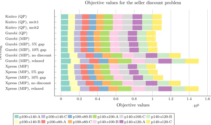
Figure 1: Sum of objective values for all tested datasets in the seller discount problem, where pA-sB-C consists of A products, B sellers in instance C. Gurobi (QP), Gurobi (MIP) and Xpress (MIP) show proven optimality. Lower values are better.
3.1.3 Implementation
Models for each solution was written inAMPL and are shown inListing 2andListing 3, underAppendix B.3
for the MIP solution and QP solution respectively.
3.1.4 Results
Figure 1 shows the sum of objective values for each solver method, allowing for an overview of how well the approximations compare to exact solutions. Table 1shows the relative accuracy of each solution, allowing for a similar comparison at greater detail. Figure 2allows for comparison of runtimes from the various methods.
The entirety of test results are shown inTable 5, underAppendix B.4.
3.1.5 Discussion
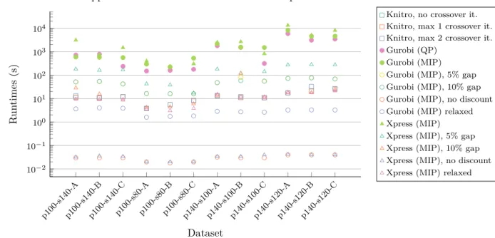
The results inFigure 2show that there is some benefit in finding global optima using theQPmodel withGurobi. The runtime improvements do however not differ by orders of magnitude, with the exception of a single tested instance. However, the difference in different solvers can affect runtimes more than the models: specifically, in instances p100-s140-A as well as p100-s140-C, Gurobi finds an optimal solution signficantly quicker than
Xpress.
Approximate solutions provide a negligible benefit for QPsolving withKnitro. In this problem, crossover iterations do not significantly impact results. As shown inFigure 1, accuracy is only slightly better thanXpress
solutions with 10% accuracy, while the runtimes do not differ significantly. Table 1shows a more fine-grained comparison between the two: the difference in accuracy for respective solutions vary by problem instance, suggesting that neither method is uniformly superior.
When relaxingMIPvariables, the model allows for mistakenly applying discounts that are invalid. This, in turn, provides highly inaccurate results. A possible solution for this would be to fine-tune the resulting solution by transferring purchases from sellers further from having their discounts applied, to those nearly reaching their discount thresholds.
3.2 Supply Restrictions
Not all sellers can be expected to provide an infinite supply. This may be reflected in a problem that restricts the size of purchases of a product from a specific seller.
Comparison of MIP and QP in Sourcing Problems Daniel Ahlbom, Uppsala University 2017
p100-s140-Ap100-s140-Bp100-s140-Cp100-s80-Ap100-s80-Bp100-s80-Cp140-s100-Ap140-s100-Bp140-s100-Cp140-s120-Ap140-s120-Bp140-s120-C 10−2 10−1 100 101 102 103 104 Dataset R un times (s)
Application runtimes for the seller discount problem
Knitro, no crossover it. Knitro, max 1 crossover it. Knitro, max 2 crossover it. Gurobi (QP)
Gurobi (MIP) Gurobi (MIP), 5% gap Gurobi (MIP), 10% gap Gurobi (MIP), no discount Gurobi (MIP) relaxed Xpress (MIP) Xpress (MIP), 5% gap Xpress (MIP), 10% gap Xpress (MIP), no discount Xpress (MIP) relaxed
Figure 2: Runtimes in seconds for all tested datasets, where pAsB-C has A products and B sellers for an instance C. Gurobi (QP), Gurobi (MIP), Xpress (MIP) found proven optimality and have filled markers. Lower values are better. The figure is provided in logarithmic scale as different methods provide results that differ in several orders of magnitude. Knitroruntimes are similar, resulting in overlaps in the figure. The same is true for the two different gap settings in Gurobi. Exact results are shown inTable 5.
Solver Settings Dataset p100-s140-A p100-s140-B p100-s140-C p100-s80-A p100-s80-B p100-s80-C p140-s100-A p140-s100-B p140-s100-C p140-s120-A p140-s120-B p140-s120-C
Knitro
None 7.24% 8.89% 9.16% 6.71% 7.40% 7.66% 6.16% 3.25% 8.14% 4.47% 6.78% 4.39% Max 1 cross it. 7.24% 8.89% 9.16% 6.71% 7.40% 7.66% 6.16% 3.25% 8.14% 4.47% 6.78% 4.39% Max 2 cross it. 5.33% 8.89% 9.16% 6.71% 7.40% 7.66% 6.16% 3.25% 8.14% 4.47% 7.05% 4.39%
Gurobi QP 0.00% 0.00% 0.00% 0.00% 0.00% 0.00% 0.00% 0.00% 0.00% 0.00% 0.00% 0.00% MIP, int. 0.00% 0.00% 0.00% 0.00% 0.00% 0.00% 0.00% 0.00% 0.00% 0.00% 0.00% 0.00% MIP, 5% gap 1.70% 0.80% 2.61% 0.19% 2.97% 2.52% 0.91% 1.50% 1.19% 2.47% 0.42% 0.78% MIP, 10% gap 1.70% 0.80% 2.61% 0.19% 2.97% 2.52% 0.91% 6.49% 1.19% 2.47% 0.42% 0.78% MIP, no disc. 26.97% 26.98% 27.35% 26.37% 26.87% 26.42% 26.24% 26.73% 27.10% 25.91% 26.05% 26.12% MIP, rel. 45.83% 46.20% 46.17% 45.35% 45.56% 45.31% 45.30% 45.81% 46.04% 44.77% 45.32% 45.16% Xpress None 0.00% 0.00% 0.00% 0.00% 0.00% 0.00% 0.00% 0.00% 0.00% 0.00% 0.00% 0.00% 5% gap 2.93% 2.87% 2.39% 0.70% 1.39% 0.16% 1.95% 1.92% 3.89% 1.76% 3.21% 2.20% 10% gap 9.98% 9.21% 7.58% 7.60% 7.89% 8.93% 8.61% 1.92% 9.44% 8.11% 7.12% 8.73% No disc. 26.97% 26.98% 27.35% 26.37% 26.87% 26.42% 26.24% 26.73% 27.10% 25.91% 26.05% 26.12% Rel. 45.83% 46.20% 46.17% 45.35% 45.56% 45.31% 45.30% 45.81% 46.04% 44.77% 45.32% 45.16% Optimal 71734.19 69054.30 69955.39 71238.80 72483.11 72426.68 100189.75 100633.70 101961.60 100100.39 102388.86 100192.48
Table 1: Accuracy of the objective values of the seller discount problem. Each cell shows how much larger the objective value of a solution is compared to the proven optimality of each dataset. An optimum solution shows exactly 0%, while larger values suggest less accuracy.
Comparison of MIP and QP in Sourcing Problems Daniel Ahlbom, Uppsala University 2017
Additionally, a seller may restrict their dependency on a specific company: another requirement restricting the total order from each seller is therefore added.
In addition to the constants defined in3.1: Seller Discounts, we add the following, including the modified array C:
• A two-dimensional array A describes the possible amount Ai,j of a product i sold by a seller j, where
Ai,j = 1 suggests the full required amount can be purchased, while Ai,j = 0 means that the seller does
not provide the product at all.
• A one-dimensional array B describes the total price Bj a seller j will accept.
3.2.1 MIP Model
We use the same decision variables as the3.1.1: MIP Modelfor3.1: Seller Discounts. This allows us to describe the problem as follows:
Minimize ∑ i∈P ∑ j∈S Ci,j· Xi,j− ∑ i∈P ∑ j∈S Di,j· Yi,j (15) Subject to ∀i ∈ P ( ∑ j∈S Xi,j≥ 1 ) (16) ∀j ∈ S( ∑ i∈P Ci,j· Xi,j− Zj· Tj ≥ 0 ) (17)
∀i ∈ P, j ∈ S(Xi,j− Yi,j≥ 0
)
(18)
∀i ∈ P, j ∈ S(Zj− Yi,j ≥ 0
)
(19)
∀i ∈ P, j ∈ S(Ai,j− Xi,j≥ 0
) (20) ∀j ∈ S(Bj− ∑ i∈P Ci,j· Xi,j≥ 0 ) (21) Where the relations define the following:
(15) is the objective, i e total cost. (16) ensures each product is ordered. (17) is the discount condition.
(18) sets that discounts are only provided for purchased products.
(19) assures discounts are only provided for a product iff the discount condition for the seller is met. (20) limits purchases according to supply: this replaces the condition whether an item is sold at all. (21) limits purchases according to permitted level.
3.2.2 QP Model
We use the same decision variables as3.1.2: QP Modelfor3.1: Seller Discounts., which describes the problem using the following statements.
Minimize ∑ i∈P ∑ j∈S D0i,j· Xi,j+ ∑ i∈P ∑ j∈S Di,j· Xi,j· Yj (22) Subject to ∀i ∈ P ( ∑ j∈S Xi,j≥ 1 ) (23) ∀j ∈ S( ∑ i∈P D0i,j· Xi,j+ ∑ i∈P Di,j· Xi,j− Tj· (1 − Yj)≥ 0 ) (24)
∀i ∈ P, j ∈ S(Ai,j− Xi,j≥ 0
) (25) ∀j ∈ S(Bj− ∑ i∈P Di,j0 · Xi,j− ∑ i∈P Di,j· Xi,j· Yj >= 0 ) (26) Where each statement considers the following:
Comparison of MIP and QP in Sourcing Problems Daniel Ahlbom, Uppsala University 2017 0 0.1 0.2 0.3 0.4 0.5 0.6 0.7 0.8 0.9 1 ·106 Knitro (QP) Knitro (QP), mcit1 Knitro (QP), mcit2 Gurobi (QP) Gurobi (MIP) Gurobi (MIP), 5% gap Gurobi (MIP), 10% gap Gurobi (MIP), no discount Xpress (MIP)
Xpress (MIP), 5% gap Xpress (MIP), 10% gap Xpress (MIP), no discount
Objective values
Setting
Objective values for the supply problem
p60-s100-A p60-s100-C p80-s60-B p100-s60-A p100-s60-C p100-s80-B p60-s100-B p80-s60-A p80-s60-C p100-s60-B p100-s80-A p100-s80-C
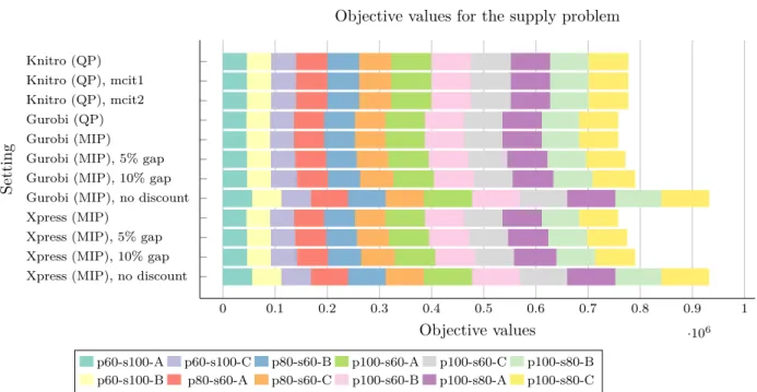
Figure 3: Sum of objective values for all tested datasets in the supply problem, where pA-sB-C consists of
A products, B sellers in instance C. Gurobi (QP), Gurobi (MIP) and Xpress (MIP) show proven optimality.
Lower values are better.
(22) is the objective, i e minimizing total cost. (23) ensures each product is ordered.
(24) is the discount condition.
(25) limits purchases according to supply: this replaces the condition whether an item is sold at all. (26) limits purchases according to permitted level.
3.2.3 Implementation
Models for each solution was written in AMPL. Models are shown in Listing 4 and Listing 5 for the MIP solution and QP solution respectively. The approximative models differ only by setting the binary variable to continuous.
3.2.4 Results
Figure 3 shows the sum of objective values for each solver method, allowing for an overview of how well the approximations compare to exact solutions. Table 2shows the relative accuracy of each solution, allowing for a similar comparison at greater detail. Figure 4allows for comparison of runtimes from the various methods.
The entirety of test results are shown inTable 6, underAppendix B.4.
3.2.5 Discussion
Similar to in 3.1: Seller Discounts, results for this problem show that solving without discounts requires siginificantly less time than finding optimal solutions, while other approximations are placed somewhere in between.
Figure 3shows that approximate solutions found withKnitroroughly correspond to objective values between the 5% and 10% gap tolerances tested with MIP solvers. Runtimes using Knitro are consistently slower than for correspondingMIPapproximations in datasets with 60 products and 100 sellers, while the opposite is true for datasets with 100 products and 80 sellers. No discernable pattern is apparent for the remaining datasets.
QPmodels inGurobiappear to be the consistently quickest way to find optimal results, with small margins in most cases.
Comparison of MIP and QP in Sourcing Problems Daniel Ahlbom, Uppsala University 2017
p60-s100-Ap60-s100-Bp60-s100-Cp80-s60-Ap80-s60-Bp80-s60-Cp100-s60-Ap100-s60-Bp100-s60-Cp100-s80-Ap100-s80-Bp100-s80-C 10−2 10−1 100 101 102 103 104 Dataset R un times (s)
Application runtimes for the supply problem
Knitro, no crossover it. Knitro, max 1 crossover it. Knitro, max 2 crossover it. Gurobi (QP)
Gurobi (MIP) Gurobi (MIP), 5% gap Gurobi (MIP), 10% gap Gurobi (MIP), no discount Xpress (MIP)
Xpress (MIP), 5% gap Xpress (MIP), 10% gap Xpress (MIP), no discount
Figure 4: Runtimes in seconds for all tested datasets, where pAsB-C has A products and B sellers for an instance C. Gurobi (QP), Gurobi (MIP), Xpress (MIP) found proven optimality and have filled markers. Lower values are better. The figure is provided in logarithmic scale as different methods provide results that differ in several orders of magnitude.
Solver Settings Dataset p60-s100-A p60-s100-B p60-s100-C p80-s60-A p80-s60-B p80-s60-C p100-s60-A p100-s60-B p100-s60-C p100-s80-A p100-s80-B p100-s80-C
Knitro
None 1.82% 2.58% 4.17% 3.84% 3.40% 5.03% 1.96% 0.74% 3.99% 0.14% 2.56% 1.83% Max 1 cross it. 1.82% 2.58% 4.17% 3.84% 3.40% 5.03% 1.96% 0.74% 3.99% 0.14% 2.56% 1.83% Max 2 cross it. 1.82% 2.58% 4.17% 3.84% 3.40% 5.03% 1.96% 0.74% 3.99% 0.14% 2.56% 1.83%
Gurobi QP 0.00% 0.00% 0.00% 0.00% 0.00% 0.00% 0.00% 0.00% 0.00% 0.00% 0.00% 0.00% MIP, int. 0.00% 0.00% 0.00% 0.00% 0.00% 0.00% 0.00% 0.00% 0.00% 0.00% 0.00% 0.00% MIP, 5% gap 2.55% 0.70% 1.89% 2.65% 0.12% 2.00% 2.78% 1.84% 0.60% 2.48% 3.33% 0.91% MIP, 10% gap 2.55% 0.70% 9.27% 2.65% 4.75% 9.35% 2.78% 1.84% 0.60% 3.77% 4.87% 9.26% MIP, no disc. 24.42% 23.53% 24.41% 22.69% 22.64% 23.76% 22.89% 22.67% 22.76% 22.30% 22.66% 22.96% Xpress None 0.00% 0.00% 0.00% 0.00% 0.00% 0.00% 0.00% 0.00% 0.00% 0.00% 0.00% 0.00% 5% gap 2.55% 0.70% 1.76% 2.65% 0.84% 2.73% 2.78% 2.93% 0.60% 2.78% 3.65% 2.55% 10% gap 2.55% 0.70% 9.27% 2.65% 8.17% 9.35% 2.78% 2.93% 0.60% 7.61% 3.65% 2.55% No disc. 24.42% 23.53% 24.41% 22.69% 22.64% 23.76% 22.89% 22.67% 22.76% 22.30% 22.66% 22.96% Optimal 44441.56 45250.31 45840.41 57937.72 58823.45 58739.54 75484.18 74694.82 74074.37 75272.57 71827.11 74792.74
Table 2: Accuracy of the objective values of the seller supply problem. Each cell shows how much larger the objective value of a solution is compared to the proven optimality of each dataset. An optimum solution shows exactly 0%, while larger values suggest less accuracy.
Comparison of MIP and QP in Sourcing Problems Daniel Ahlbom, Uppsala University 2017
3.3
Regional Division
Ordering products from a seller brings some overhead: an optimized minimum cost may result in an impractical number of sellers to manage.
This problem is of particular interest when a company requires purchases to be made for a larger amount of regions: for example, a small number of national sellers can be more managable than a large number of local sellers. This is, however, not always a possibility: for example, there may be a policy that requires a certain class of wares to be locally produced.
Another interpretation may be in a multinational context: global corporations may deliver products to certain countries, but not all.
The problem can be defined according to the following constants: • Let set P represent all products such that P ={i ∈ N | 1 ≤ i ≤ |P |}.
• Let set S represent all sellers such that S ={j ∈ N | 1 ≤ j ≤ |S|}. • Let set R represent all regions such that R ={k ∈ N | 1 ≤ k ≤ |R|}.
• A three-dimensional array C∈ R|P |×|S|×|R| describes cost Ci,j,kfor product i when provided by seller j,
where Ci,j,k> 0. If seller i does not provide product i, the cost is set to Ci,j,k=−1.
• A three-dimensional array D ∈ R|P |×|S|×|R| describes the possible discount Di,j,k for product i when
provided by seller j, where Di,j,k> 0.
• A three-dimensional array D0 = C − D describes the discounted price for each product, such that each element Di,j,k0 = Ci,j,k− Di,j,k.
• A two-dimensional array Q of size|P | × |R| describes the number of units Qi,k required of a product i in
region k. If Qi,j = 0, the product is not required in this region.
• A one-dimensional array L of size|R| describes the limit Lk of total sellers serving a single region k.
• A constant l describes the total amount of sellers allowed across all regions.
3.3.1 MIP Model
We use decision variables similar to the 3.1.1: MIP Modelfor3.1: Seller Discounts.
• A three-dimensional array X∈ R|P |×|S|×|R| of real values 0≤ Xi,j where Xi,j,kis the ordered amount of
product i from seller j in region k.
• A three-dimensional array Y∈ R|P |×|S|×|R| of real values 0≤ Y
i,j where Yi,j,k = Xi,j,k if the discount
is applied for seller j and product i is purchased from them in region k. • A one-dimensional array Z∈ N|S| of binary values Z
j ∈ {0, 1} where Zj = 1 if the discount is applied for
seller j.
• A two-dimensional array U∈ N|S|×|R| of binary values Uj,k ∈ {0, 1} where Uj,k = 1 if seller j has an
order in region k.
• A one-dimensional array V∈ N|S| of binary values Vj∈ {0, 1} where Vj = 1 if seller j has any order.
Comparison of MIP and QP in Sourcing Problems Daniel Ahlbom, Uppsala University 2017 Minimize ∑ i∈P ∑ j∈S ∑ k∈R Ci,j,k· Xi,j,k− ∑ i∈P ∑ j∈S ∑ k∈R Di,j,k· Yi,j,k (27) Subject to ∀i ∈ P, ∀k ∈ R( ∑ j∈S Xi,j,k− Qi,k ≥ 0 ) (28) ∀j ∈ S( ∑ i∈P ∑ k∈R Ci,j,k· Xi,j,k− Zj· Tj ≥ 0 ) (29)
∀i ∈ P, j ∈ S, k ∈ R(Xi,j,k− Yi,j,k≥ 0
)
(30)
∀i ∈ P, j ∈ S(Qi,k· Zi,j− Yi,j,k≥ 0
)
(31)
∀i ∈ P, j ∈ S, k ∈ R(Ci,j,k· Xi,j,k≥ 0
)
(32)
∀i ∈ P, j ∈ S, k ∈ R(Uj,k· Qi,k− Xi,j,k≥ 0
) (33) ∀k ∈ R( ∑ j∈S Uj,k− Lk≤ 0 ) (34) ∀j ∈ S, k ∈ R(Vj− Uj,k≥ 0 ) (35) ∀j ∈ S(Vj− l ≤ 0 ) (36) Where the relations define the following:
(27) is the objective, i e total cost. (28) ensures each product is ordered. (29) is the discount condition.
(30) sets that discounts are only provided for purchased products.
(31) assures discounts are only provided for a product iff the discount condition for the seller is met. (32) sets that purchases can only be made when a seller provides the product.
(33) sets whether a seller has an order in a region. (34) limits sellers in a region.
(35) sets whether a seller has any order. (36) limits total number of sellers.
3.3.2 QP Model
We use decision variables similar to the 3.1.2: QP Modelfor3.1: Seller Discounts.
• A three-dimensional array X∈ R|P |×|S|×|R| of real values 0≤ Xi,j where Xi,j,kis the ordered amount of
product i from seller j in region k.
• A one-dimensional array Y∈ N|S|of binary values Yj∈ {0, 1} where Yj = 1 if the discount is not applied
for seller j.
• A two-dimensional array U∈ N|S|×|R| of binary values U
j,k ∈ {0, 1} where Uj,k = 1 if seller j has an
order in region k.
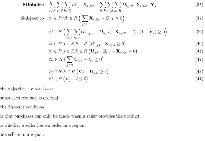
Comparison of MIP and QP in Sourcing Problems Daniel Ahlbom, Uppsala University 2017 Minimize ∑ i∈P ∑ j∈S ∑ k∈R Di,j0 · Xi,j,k+ ∑ i∈P ∑ j∈S ∑ k∈R Di,j,k· Xi,j,k· Yj (37) Subject to ∀i ∈ P, ∀k ∈ R( ∑ j∈S Xi,j,k− Qi,k≥ 0 ) (38) ∀j ∈ S( ∑ i∈P ∑ k∈R
(Di,j,k0 + Di,j,k)· Xi,j,k− Tj· (1 − Yj)≥ 0
)
(39)
∀i ∈ P, j ∈ S, k ∈ R(D0i,j,k· Xi,j,k≥ 0
)
(40)
∀i ∈ P, j ∈ S, k ∈ R(Uj,k· Qi,k− Xi,j,k≥ 0
) (41) ∀k ∈ R( ∑ j∈S Uj,k− Lk ≤ 0 ) (42) ∀j ∈ S, k ∈ R(Vj− Uj,k≥ 0 ) (43) ∀j ∈ S(Vj− l ≤ 0 ) (44) (37) is the objective, i e total cost.
(38) ensures each product is ordered. (39) is the discount condition.
(40) sets that purchases can only be made when a seller provides the product. (41) sets whether a seller has an order in a region.
(42) limits sellers in a region.
(43) sets whether a seller has any order. (44) limits total number of sellers.
3.3.3 Implementation
Models for each solution were written inAMPL. The models are shown inListing 6andListing 7for the MIP solution and QP solution respectively. The approximative models differ only by setting the binary variable to continuous.
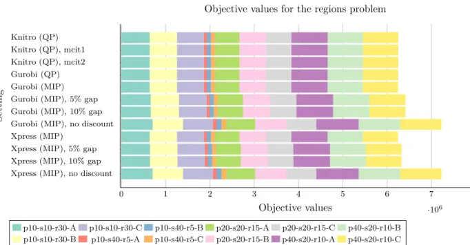
3.3.4 Results
Figure 5 show the sum of objective values for each solver method, allowing for an overview of how well the approximations compare to exact solutions. Figure 6 allows for comparison of runtimes from the various methods.
The entirety of test results are shown inTable 7, underAppendix B.4.
3.3.5 Discussion
In this subproblem, theQP modelperforms unevenly withGurobi, in comparison with the other tested methods for finding optimal solutions, while the QP model performs significantly slower with Knitro than all other configurations, including all three set-ups finding proven optimality.
In contrast with experiments in both 3.1: Seller Discountsand 3.2: Supply Restrictions, Knitrodoes find solutions very close to optimality, even when compared toMIPconfigurations with 5% and 10% gap tolerances. Since QP algorithms have a tendency to become inefficient for a large number of variables [5], it is possible that the three-dimensional arrays constructed for this problem cause the longer runtimes. Meanwhile, Gurobi
andXpressare likely able to use conventionalMIPalgorithms, handling larger variable arrays with less issues. Further, they are likely to exploit the restricted amounts of sellers, which further cuts down the search space. TheQPmodel used withGurobistill shows comparable, but not superior, runtimes for optimal solutions.
Comparison of MIP and QP in Sourcing Problems Daniel Ahlbom, Uppsala University 2017 0 1 2 3 4 5 6 7 ·106 Knitro (QP) Knitro (QP), mcit1 Knitro (QP), mcit2 Gurobi (QP) Gurobi (MIP) Gurobi (MIP), 5% gap Gurobi (MIP), 10% gap Gurobi (MIP), no discount Xpress (MIP)
Xpress (MIP), 5% gap Xpress (MIP), 10% gap Xpress (MIP), no discount
Objective values
Setting
Objective values for the regions problem
p10-s10-r30-A p10-s10-r30-C p10-s40-r5-B p20-s20-r15-A p20-s20-r15-C p40-s20-r10-B p10-s10-r30-B p10-s40-r5-A p10-s40-r5-C p20-s20-r15-B p40-s20-r10-A p40-s20-r10-C
Figure 5: Sum of objective values for all tested datasets in the regions problem, where pA-sB-C consists of
A products, B sellers in instance C. Gurobi (QP), Gurobi (MIP) and Xpress (MIP) show proven optimality.
Lower values are better.
p10-s10-r30-Ap10-s10-r30-Bp10-s10-r30-Cp10-s40-r5-Ap10-s40-r5-Bp10-s40-r5-Cp20-s20-r15-Ap20-s20-r15-Bp20-s20-r15-Cp40-s20-r10-Ap40-s20-r10-Bp40-s20-r10-C 10−2 10−1 100 101 102 103 104 Dataset R un times (s)
Application runtimes for the regions problem
Knitro, no crossover it. Knitro, max 1 crossover it. Knitro, max 2 crossover it. Gurobi (QP)
Gurobi (MIP) Gurobi (MIP), 5% gap Gurobi (MIP), 10% gap Gurobi (MIP), no discount Xpress (MIP)
Xpress (MIP), 5% gap Xpress (MIP), 10% gap Xpress (MIP), no discount
Figure 6: Runtimes in seconds for all tested datasets, where pAsB-C has A products and B sellers for an instance C. Gurobi (QP), Gurobi (MIP), Xpress (MIP) found proven optimality and have filled markers. Lower values are better. The figure is provided in logarithmic scale as different methods provide results that differ in several orders of magnitude.
Comparison of MIP and QP in Sourcing Problems Daniel Ahlbom, Uppsala University 2017
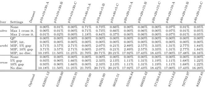
Solver Settings Dataset p10-s10-r30-A p10-s10-r30-B p10-s10-r30-C p10-s40-r5-A p10-s40-r5-B p10-s40-r5-C p20-s20-r15-A p20-s20-r15-B p20-s20-r15-C p40-s20-r10-A p40-s20-r10-B p40-s20-r10-C
Knitro
None 0.00% 0.01% 0.00% 0.71% 0.73% 0.66% 0.00% 0.06% 0.00% 0.07% 0.01% 0.05% Max 1 cross it. 0.00% 0.01% 0.00% 0.71% 0.73% 0.66% 0.00% 0.06% 0.00% 0.07% 0.01% 0.05% Max 2 cross it. 0.01% 0.02% 0.00% 1.18% 0.84% 0.37% 0.00% 0.06% 0.00% 0.07% 0.01% 0.05%
Gurobi QP 0.00% 0.00% 0.00% 0.00% 0.00% 0.00% 0.00% 0.00% 0.00% 0.00% 0.00% 0.00% MIP, int. 0.00% 0.00% 0.00% 0.00% 0.00% 0.00% 0.00% 0.00% 0.00% 0.00% 0.00% 0.00% MIP, 5% gap 3.71% 3.57% 2.71% 0.00% 2.07% 0.21% 2.89% 2.57% 3.33% 1.31% 2.77% 1.84% MIP, 10% gap 3.71% 3.57% 2.71% 0.00% 2.07% 0.21% 2.89% 2.57% 3.33% 1.31% 2.77% 1.84% MIP, no disc. 10.19% 11.50% 11.25% 21.70% 20.71% 20.21% 17.92% 17.43% 18.43% 17.00% 17.48% 16.16% Xpress None 0.00% 0.00% 0.00% 0.00% 0.00% 0.00% 0.00% 0.00% 0.00% 0.00% 0.00% 0.00% 5% gap 0.93% 0.90% 1.66% 0.00% 2.33% 2.13% 1.11% 1.31% 1.19% 1.11% 1.68% 1.22% 10% gap 0.93% 0.90% 1.66% 0.00% 2.33% 2.13% 1.11% 1.31% 1.19% 1.11% 1.68% 1.22% No disc. 10.18% 11.50% 11.25% 21.70% 20.71% 20.21% 17.92% 17.43% 18.42% 17.00% 17.43% 16.20% Optimal 633951.12 615860.60 610585.91 67197.00 89291.00 90525.51 553186.84 600235.42 571204.63 817514.62 797792.97 842267.85
Table 3: Accuracy of the objective values of the regions problem. Each cell shows how much larger the objective value of a solution is compared to the proven optimality of each dataset. An optimum solution shows exactly 0%, while larger values suggest less accuracy.
3.4
Reserved Price
A special case appears where the number of sellers a customer will order from is highly limited.
Consider a situation where a customer will purchase a number of products from one of two sellers. The first provides highly competitive prices for all products but one, which may be unavailable or sold at a very high cost. The other seller provides all products, but all are at a significantly higher price. In this case, a customer may want to consider ordering the competitively priced products from the first seller, while ordering the very last product by some other means.
To implement this problem, a reserved price is introduced. For each product such that, if the total cost will be lowered by purchasing a product of this price, it is applied without increasing the number of sellers from which an order is made.
In addition to the constants defined in3.1: Seller Discounts, the following constants are defined. • A seller limit l that sets the highest total number of sellers.
• A one-dimensional array H of size P , where each entry Hiis the penalty, or reserved price, for not ordering
a product from any of the defined sellers.
3.4.1 MIP Model
We use the same decision variables as the 3.1.1: MIP Model for3.1: Seller Discounts, with the following two additions.
• A one-dimensional array V∈ N|S| of binary values Vj∈ {0, 1} where Vj = 1 if seller j has any order.
• A one-dimensional array W∈ R|P | of real values 0≤ Wi≤ 1 where Wj ≥ 0 if a product is ordered from
a different source.
Comparison of MIP and QP in Sourcing Problems Daniel Ahlbom, Uppsala University 2017 Minimize ∑ i∈P Wi· Hi+ ∑ i∈P ∑ j∈S Ci,j· Xi,j− ∑ i∈P ∑ j∈S Di,j· Yi,j (45) Subject to ∀i ∈ P (Wi+ ∑ j∈S Xi,j≥ 1 ) (46) ∀j ∈ S( ∑ i∈P Ci,j· Xi,j− Tj· Zj≥ 0 ) (47)
∀i ∈ P, j ∈ S(Xi,j− Yi,j≥ 0
)
(48)
∀i ∈ P, j ∈ S(Zj− Yi,j≥ 0
)
(49)
∀i ∈ P, j ∈ S(Ci,j· Xi,j≥ 0
) (50) ∀i ∈ P, ∀j ∈ S(Vj− Xi,j≥ 0 ) (51) ∑ j∈S Vj− l ≤ 0 (52)
Where the relations define the following: (45) is the objective, i e total cost.
(46) ensures each product is ordered. (47) is the discount condition.
(48) sets that discounts are only provided for purchased products.
(49) assures discounts are only provided for a product iff the discount condition for the seller is met. (50) sets that purchases can only be made when a seller provides the product.
(51) sets whether a seller has any order. (52) limits total number of sellers.
3.4.2 QP Model
We use the same decision variables as the 3.1.2: QP Model for3.1: Seller Discounts, with the following two additions.
• A one-dimensional array V∈ N|S| of binary values Vj∈ {0, 1} where Vj = 1 if seller j has any order.
• A one-dimensional array W∈ R|P | of real values 0≤ Wi≤ 1 where Wj ≥ 0 if a product is ordered from
a different source. Minimize ∑ i∈P Hi· Wi+ ∑ i∈P ∑ j∈S Di,j0 · Xi,j+ ∑ i∈P ∑ j∈S Di,j· Xi,j· Yj (53) Subject to ∀i ∈ P (Wi ∑ j∈S Xi,j≥ 1 ) (54) ∀j ∈ S( ∑ i∈P D0i,j· Xi,j+ ∑ i∈P Di,j· Xi,j− Tj· (1 − Yj)≥ 0 ) (55)
∀i ∈ P, j ∈ S(Di,j0 · Xi,j≥ 0
) (56) ∀i ∈ P, j ∈ S(Vj− Xi,j≥ 0 ) (57) ∑ j∈S Vj− l ≤ 0 (58)
(53) is the objective, i e total cost. (54) ensures each product is ordered. (55) is the discount condition.
(56) sets that purchases can only be made when a seller provides the product. (57) sets whether a seller has any order.
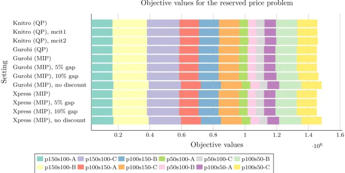
Comparison of MIP and QP in Sourcing Problems Daniel Ahlbom, Uppsala University 2017 0.2 0.4 0.6 0.8 1 1.2 1.4 1.6 ·106 Knitro (QP) Knitro (QP), mcit1 Knitro (QP), mcit2 Gurobi (QP) Gurobi (MIP) Gurobi (MIP), 5% gap Gurobi (MIP), 10% gap Gurobi (MIP), no discount Xpress (MIP)
Xpress (MIP), 5% gap Xpress (MIP), 10% gap Xpress (MIP), no discount
Objective values
Setting
Objective values for the reserved price problem
p150s100-A p150s100-C p100s150-B p50s100-A p50s100-C p100s50-B p150s100-B p100s150-A p100s150-C p50s100-B p100s50-A p100s50-C
Figure 7: Sum of objective values for all tested datasets in the reserved price problem, where pA-sB-C consists of A products, B sellers in instance C. Gurobi (QP), Gurobi (MIP) and Xpress (MIP) show proven optimality. Lower values are better.
3.4.3 Implementation
Models for each solution were written inAMPL. The models are shown inListing 8andListing 9for the MIP solution and QP solution respectively.
3.4.4 Results
Figure 7 shows the sum of objective values for each solver method, allowing for an overview of how well the approximations compare to exact solutions. Table 4shows the relative accuracy of each solution, allowing for a similar comparison at greater detail. Figure 8allows for comparison of runtimes from the various methods.
Full results are shown inTable 8.
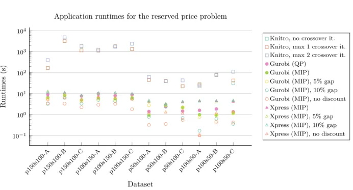
3.4.5 Discussion
Similarly to observations in3.3.5: Discussion, results forGurobiandXpressare favorable to those ofKnitro. WhileQP withKnitro configurations consistently provides results near optimality, runtimes exceed those ofGurobiandXpressby orders of magnitude in all tested datasets. Notably, allowing for 2 crossover iterations provides worse objective values – this may be explained by a floating point error. Further, approximations used with MIP configurations provide similarly promising results at even more improved runtimes. QP and MIP
configurations inGurobiprovide generally similar runtimes, where the advantage varies by each dataset. Overall, this problem suggests thatQPandMIPconfigurations are similarly powerful usingGurobi, while
Comparison of MIP and QP in Sourcing Problems Daniel Ahlbom, Uppsala University 2017
p150s100-Ap150s100-Bp150s100-Cp100s150-Ap100s150-Bp100s150-Cp50s100-Ap50s100-Bp50s100-Cp100s50-Ap100s50-Bp100s50-C 10−1 100 101 102 103 104 Dataset R un times (s)
Application runtimes for the reserved price problem
Knitro, no crossover it. Knitro, max 1 crossover it. Knitro, max 2 crossover it. Gurobi (QP)
Gurobi (MIP) Gurobi (MIP), 5% gap Gurobi (MIP), 10% gap Gurobi (MIP), no discount Xpress (MIP)
Xpress (MIP), 5% gap Xpress (MIP), 10% gap Xpress (MIP), no discount
Figure 8: Runtimes in seconds for all tested datasets, where pAsB-C has A products and B sellers for an instance C. Gurobi (QP), Gurobi (MIP), Xpress (MIP) found proven optimality and have filled markers. Lower values are better. The figure is provided in logarithmic scale as different methods provide results that differ in several orders of magnitude.
Solver Settings Dataset p150s100-A p150s100-B p150s100-C p100s150-A p100s150-B p100s150-C p50s100-A p50s100-B p50s100-C p100s50-A p100s50-B p100s50-C
Knitro
None 0.00% 0.00% 0.92% 0.54% 0.00% 0.05% 0.00% 0.00% 0.00% 0.94% 0.00% 0.00% Max 1 cross it. 0.00% 0.00% 0.92% 0.54% 0.00% 0.05% 0.00% 0.00% 0.00% 0.94% 0.00% 0.00% Max 2 cross it. 1.13% 0.00% 1.24% 0.00% 0.00% 0.05% 0.99% 0.00% 0.00% 0.94% 0.00% 0.00%
Gurobi QP 0.00% 0.00% 0.00% 0.00% 0.00% 0.00% 0.00% 0.00% 0.00% 0.00% 0.00% 0.00% MIP, int. 0.00% 0.00% 0.00% 0.00% 0.00% 0.00% 0.00% 0.00% 0.00% 0.00% 0.00% 0.00% MIP, 5% gap 0.00% 0.00% 0.00% 0.00% 0.00% 0.00% 0.00% 0.00% 0.00% 0.03% 0.00% 0.00% MIP, 10% gap 0.00% 0.00% 0.00% 0.00% 0.00% 0.00% 0.00% 0.00% 0.00% 8.86% 2.63% 0.00% MIP, no disc. 3.89% 2.37% 0.26% 1.90% 0.75% 1.29% 1.23% 6.41% 0.18% 4.40% 4.00% 0.66% Xpress None 0.00% 0.00% 0.00% 0.00% 0.00% 0.00% 0.00% 0.00% 0.00% 0.00% 0.00% 0.00% 5% gap 0.00% 0.00% 0.00% 0.00% 0.00% 0.00% 0.00% 0.00% 0.00% 0.00% 0.00% 0.00% 10% gap 0.00% 0.00% 0.00% 0.00% 0.00% 0.00% 0.00% 0.00% 0.00% 0.00% 0.00% 0.00% No disc. 3.89% 2.37% 0.26% 1.90% 0.75% 1.29% 1.23% 6.41% 0.18% 3.49% 4.00% 0.66% Optimal 162661.05 216974.92 203646.79 122473.65 126080.31 129088.76 54149.66 52328.36 51603.81 71238.31 134949.40 127011.46
Table 4: Accuracy of the objective values of the reserved price problem. Each cell shows how much larger the objective value of a solution is compared to the proven optimality of each dataset. An optimum solution shows exactly 0%, while larger values suggest less accuracy.
Summary Daniel Ahlbom, Uppsala University 2017
4 Summary
4.1 Conclusion
Test results show thatQPprovides no significant benifit overMIPin solving the presented problems, with the used parameters.
Solversexploiting the binary nature of variables, allowing for finding optimal solutions in non-convex prob-lems, have lead to slightly increased efficiency in the experiments outlined in 3.1: Seller Discounts as well as
3.2: Supply Restrictions. In the following two experiments, results have been less consistent.
Approximate solutions provide several considerations. GurobiandXpressallow for relaxing integer variables inMIP models, while relaxed integer variables inQP modelswere only allowed inKnitrofor the tested problems. Further, the non-convex nature of the discussed problems do not allow for globally optimal solutions in QP
models inKnitro, such that the solutions become locally optimal – essentially becoming approximations. These solutions have generally been comparable to applying an optimality gap between 5% and 10% in Gurobiand
Xpress. The significant caveat in this case, however, is that no such gap can be guaranteed for general, non-convex QPproblems. Considering runtimes,QPmodels inKnitro appear to perform similarly to comparable
MIP approximations at best, while being consistently and significantly slower at worst. The latter is certainly the case in experiments discussed in3.3: Regional Divisionand3.4: Reserved Price.
There are, however, many nuances to consider. For example, amodelwritten in terms ofQPmay be more intuitively formulated and understood. If, for example, multiplication of binary variables is performed, a QP
model appears to be likely to perform similarly to MIP model in finding a solution that is optimal, as shown in all four discussed problems, or within an increased global optimality gap. It may however be cumbersome to consider the limitations of what a solver allows for: at the time of writing,Xpressonly accepts convexQP
unless all variables are restricted to binary values [9].
To summarize, it appears that for the discussed problems and solvers, it is possible to write efficientMIP
models that allow for finding solutions that are, at worst, nearly as good in terms of runtimes and optimality as QP.
4.2
Future Work
Since there are a large amount of untestedsolvers, testing them all would be far beyond the scope of this report. Research inQPalgorithms is being done continuously, which may quickly provide an advantage tosolvers
implementing the latest discoveries, while the same is true for MIP solvers. As such, the results found in this report may drastically differ in future versions of the same software. Generally, all testedsolversare considered state-of-the-art, suggesting that they incorporate what may be considered leading edge research. Since the software is proprietary, the details of their implementations are difficult to assess. Further, entirely different technologies such as constraint programming and local search allow for finding approximations and optimal solutions as well: since these are being continuously researched in a similar manner, considering the quality of these solvers could provide interesting results as well.
Further experimentation withmodels and parameters could also provide significant benefits. It is difficult to prove whether a specific implementation of a problem is most efficient, in any aspect, as unknown approaches may exist. The impact of setting different parametres may also provide interesting results: the tested solvers
allow for a multitude of settings that can be used in a large number of combinations.
The problems discussed in this report do not cover the entirety of strategic sourcing. Any combination of the applied considerations may be used to create new sets of constraints. Further, entirely different constraints may be applied for penalizing factors such as environmental impact.
In conclusion, while this report shows thatQP does not appear to provide any significant benefit for the discussed problems, it is by no means to be considered exhaustive.
References Daniel Ahlbom, Uppsala University 2017
References
[1] Sandholm T, Levine D, Concordia M, Martyn P, Hughes R, Jacobs J, et al. Changing the Game in Strategic Sourcing at Procter & Gamble: Expressive Competition Enabled by Optimization. Interfaces. 2006;36(1):55–68. Available from: http://www.jstor.org/stable/20141360.
[2] Beall S, Carter C, Carter PL, Germer T, Hendrick T, Jap S, et al. The role of reverse auctions in strategic sourcing. CAPS research. 2003;.
[3] Cormen TH, Leiserson CE, Rivest RL, Stein C. Introduction to Algorithms. 3rd ed. Cambridge, MA: MIT Press; 2009.
[4] Eén N, Sörensson N. An extensible SAT-solver. In: International conference on theory and applications of satisfiability testing. Springer; 2003. p. 502–518.
[5] Nocedal J, Wright SJ. Numerical optimization. 2nd ed. New York: Springer; 2006.
[6] Luenberger DG, Ye Y. Linear and Nonlinear Programming. 4th ed. Cham: Springer International Pub-lishing; 2016.
[7] Byrd R, Nocedal J, Waltz R. Knitro: An Integrated Package for Nonlinear Optimization. Large-scale nonlinear optimization. 2006;p. 35–59.
[8] Wächter A, Biegler LT. Failure of global convergence for a class of interior point methods for nonlinear programming. Mathematical Programming. 2000;88(3):565–574.
[9] Bussieck MR, Vigerske S. MINLP solver software. Wiley encyclopedia of operations research and man-agement science. 2010;.
[10] Fourer R, Gay DM, Kernighan BW. A modeling language for mathematical programming. Management Science. 1990;36(5):519–554.