2012, Lund Lund University Lund Institute of Technology Division of Production Management Department of Industrial Management and Logistics
Benefits of Multi-Echelon Inventory Control
A case study at Tetra Pak
Author: Oskar Räntfors
Supervisors: Johan Marklund, LTH Jonas Schmidt
ABSTRACT
This thesis studies a two-echelon distribution inventory system with a central depot which supplies N non-identical retailers with a single product. Stochastic customer demand occurs solely at the retailers. The purpose of the master thesis project is to evaluate the potential benefit of two methods in which the control of the inventory points in the inventory system is coordinated. The two models of coordinated control are benchmarked against a widely used single stage (uncoordinated) method.
Comparisons of the solutions produced by the methods are done using a discrete event simulation model based on real inventory data. The effectiveness of the models are evaluated in terms of the resulting total system cost, the average inventory levels, and different types of service levels.
The simulation results clearly indicate that the evaluated methods for coordinated control of inventories can offer considerable savings in reduced inventory levels and even, in many cases, at the same time increasing the fill rate. The reductions in total cost range 11-37% and an increase in fill rate accompanied by a reduction of the holding costs is observed in most cases. Especially the holding costs at the Central Warehouse can be reduced; when using a method for coordinated control the fill rate for orders from the retailers is 16-71% which corresponds to a reduction of the CW holding costs of 50-94%.
FOREWORD
This master thesis is the concluding chapter of my journey to become a Master of Science in Industrial Engineering. The project has been done in collaboration with an ERP systems supplier who wishes to remain anonymous and Tetra Pak Technical Services who wanted to know more about coordinated control in multi-echelon inventory systems. For me, this has been a very rewarding journey, the analytical skills I have absorbed during my four years at Lund Institute of Technology has been tested to the maximum.
A would like to take this opportunity to thank my supervisor Johan Marklund at LTH, his help and support has been essential for this master thesis. I would also like to thank all of you that was always helpful and provided important input at the anonymous ERP systems supplier, you know who you are. A special thank goes to Jörgen Siversson at Tetra Pak for supplying the crucial inventory data. I am also grateful to Christian Howard for supplying me with his Extend model.
CONTENTS
1. INTRODUCTION ... 1
1.1. Background to inventory control in a multi-echelon system ... 1
1.2. The studied inventory system and methods for coordinated control ... 3
1.3. Problem definition ... 5
1.4. Method ... 6
1.5. Outline of the report ... 7
2. THEORETICAL FRAMEWORK ... 8
2.1. Inventory control theory ... 8
2.1.1. Concepts ... 8
2.1.2. Normally distributed demand ... 10
2.1.3. Poisson process ... 10
2.1.4. Compound poisson demand ... 11
2.1.5. Gamma distribution... 12
2.1.6. Optimal reorder points for an continuous review (R, Q) policy ... 14
2.2. Multi-echelon inventory systems ... 17
2.2.1. Uncoordinated control of multi-stage inventory systems ... 18
2.3. Coordinated multi-echelon inventory optimization methods ... 19
2.3.1. The considered multi-echelon models - preliminaries ... 19
2.3.2. Model 1: Heuristic coordination of a decentralized inventory systems using induced backorder costs ... 21
2.3.3. Model 2: Approximate optimization of a two-echelon distribution inventory system 26 3. METHOD OF EVALUATION ... 30
3.1. Simulation model ... 30
3.2. Selecting test cases ... 31
3.3. Supply in-data for the simulation ... 32
3.3.1. Virtual retailer ... 34
3.3.2. Calculate reorder levels ... 34
3.4. Output data analysis ... 35
4. RESULTS AND DISCUSSION ... 36
4.2. Sensitivity analysis ... 40
4.2.1. Eliminate direct upstream demand ... 40
4.2.2. Demand mean, transporting times and batch quantities ... 42
4.2.3. Target service levels ... 47
4.2.4. Homogenous / Heterogenic demand structure ... 48
5. CONCLUSIONS AND FUTURE RESEARCH ... 51
6. Appendix ... 53 6.1. Appendix A ... 53 6.2. Appendix B... 54 6.3. Appendix C ... 56 6.4. Appendix E ... 57 References ... 61
1.
INTRODUCTION
Supply Chain Management, the control of the material flow from suppliers of raw material to final customers, is today widely recognized as a crucial activity in most enterprises. The interest in coordinated control of multi-stage inventory systems in most supply chains is growing rapidly. A reason for this is that during the last two decades the research in this area has progressed substantially; many early models, which were rather restrictive in their assumptions, have been replaced by quite general ones. The new information technology has also greatly increased the possibilities for effective use of these models. Still, in practice today, there are very few examples of applications of the new research even though multi-echelon systems are common. This can be explained by the fact that the methods are quite difficult to understand and there are few illustrations of the benefits that coordinated control may bring in real cases. This master thesis aims to provide such an illustration by evaluating newly researched methods for coordinated inventory control using a simulation model based on real inventory data.
This study was initiated by an ERP system supplier who wishes to remain anonymous, and the inventory data required for the simulation models was acquired from Tetra Pak
Technical Services. Tetra Pak Technical Services provide technical expertise, services and support in the areas of food processing and food packaging. They offer installation and start-up services at a new plant; customized solutions within maintenance, verification, and parts together with improvement services to enhance the performance; they also offer training services for operators, maintenance personnel and managers. The inventory system in question has its central warehouse in Lund and is handling spare parts for food processing and packaging machinery.
1.1. Background to inventory control in a multi-echelon system A multi-stage, or multi-echelon, inventory system, consists of two or more inventory locations that are connected to each other. In a multi-echelon distribution system each location has as most one predecessor but an arbitrarily number of successors. The
complexities of managing inventory for such system increases significantly compared to the single-echelon case.
Figure 1.1 A single-echelon inventory system and a two-echelon distribution system. Before indulging in the challenges of multi-echelon systems let us review the single-echelon problem, as seen in Figure 1.1. To control this inventory system one must make decisions about which items to stock; how much stock to keep on hand; how often to inspect the inventory; when to buy; how much to buy; controlling pilferage and damage; and managing shortages and back orders. This is what inventory control is about and the ultimate
objective is to reduce the cost of the distribution, taking into account both costs associated with keeping products in stock, holding costs, and costs associated with not being able to satisfy customer demand directly, shortage costs. To narrow the scope of this master thesis the focus lies on one of these questions: When to buy? A common way to answer this question is to use the (R, Q) policy. This policy implies that a batch of Q units is ordered when the inventory position (stock on hand + outstanding orders – backorders) drops to, or below, the reorder point of R units. Therefore, to set a value for R is to answer the
question of when to replenish. By assuming continually inspected inventories (the time between inspections is zero) the question on when to order is answered. The approaches for finding an optimum ordering policy is well known for the single echelon case (Axsäter, 2006), they depend on a series of factors:
- Demand forecast.
- Leadtime to the external supplier - Service level goal
But how should you set the control variables in the multi-echelon case? Today, enterprises typically apply the single-echelon approach to each stock point in the system without explicitly considering how decisions at one stock point affects the others; we refer to this as an uncoordinated control of a multi-echelon system. Two questions arise:
- How much stock should be kept at the warehouse and at the different retailers? - How do shortages at the warehouse affect the retailer leadtime?
The two questions are related, they have to do with the dynamics of the system; if you reduce the service level of the warehouse, the risk of shortages will increase and therefore the risk that an order from a retailer is delayed. As a result, the average retailer leadtime will increase. Since those dynamics are impossible to take into account when the coupled inventories are treated as independent there is no scientific way to determine the warehouse service level. The uncoordinated approach will thus result in suboptimal solutions often with excess inventory.
We now turn to the more advanced methods for control of multi-echelon inventory systems, which we refer to as methods for coordinated control. There exists no completely general method that works in all types of systems. The method depends on the
characteristics of the inventory system in question, such as: The physical properties of the system, i.e., how the installations are coupled to each other, the size of the system, for example, larger systems with high demand generally require approximate methods, as exact methods tend to be computationally very demanding. Another aspect that governs the choice of model is whether the system is controlled centralized or decentralized. For an introduction on multi-echelon theories see Axsäter’s Inventory Control (2006).
1.2. The studied inventory system and methods for coordinated control The considered inventory system is a two-level distribution system, which consists of one central warehouse to which an arbitrarily number of retailers, N, are connected, see Figure 1.1. Customer demand takes place at the retailers, which replenish their stock from the warehouse. The warehouse in turn places its orders with an outside supplier. The
fully backordered. This means that in case of a stock-out the customer waits until the demand is fulfilled. Deliveries are made on a first-come first-serve basis – i.e. demand is satisfied in the order it arrives. Transportation times are constant but retailer leadtimes are stochastic due to possible shortages at the warehouse. All facilities use continuous review (R,Q)-policies. This means that when the local inventory position (stock on hand + outstanding orders – backorders) at the facility i decline to or below Ri, a replenishment
order of Qi units is placed. The objective is to optimize the reorder points Ri, i=0, 1, 2 …
N (0 corresponds to the central warehouse), the batch quantity and other inventory parameters are given and fixed. Also, indications are that to assume predetermined and fixed order quantities will only have a marginal effect on the expected cost, provided that the reorder cost is adjusted accordingly and that the given order quantities are not too far off, see for example Zheng (1992) and Axsäter (1996).
The two multi-echelon methods chosen to be evaluated in this study are both developed at the division of production management at Lund Institute of Technology. The first method, which will be denoted as Method 1 in the report, is the result from a series of three
publications. The first article (Andersson et al. 1998) introduces an induced backorder cost at the warehouse, which will reflect the impact of the warehouse reorder level on the retailer leadtime, and ultimately the end-customer service level. A somewhat
computationally demanding iterative procedure is used to find an optimal value for the induced backorder cost. The introduction of the induced backorder cost enables a
decomposition of the multi-echelon system into a number of single echelon problems. The model is based on a simple approximation, in which the stochastic leadtimes perceived by the retailers are replaced by their correct averages. The method also assumes identical order quantities at the retailers and normally distributed end customer demand. The second article (Andersson & Marklund 2000) lifts the restriction of identical retailers. The third (Berling & Marklund 2006) uses the iterative procedure developed in the first article to build an intuitive understanding as to how the optimal induced backorder cost depends on the system parameters, and uses this knowledge to create simple closed-form estimates of the induced backorder, thus eliminating the computationally demanding iterative process in the earlier publications.
The second method is based on Axsäter (2003), it is denoted as Method 2 in the report. It uses normal approximations both for the retailer demand and the demand at the
warehouse, i.e., orders from the retailers. The normal approximations make it possible to optimize even quite large systems effectively. The method also assumes that the mean and variance for the delay at the warehouse, due to shortages, is the same for all retailers. The general idea of the method is to (1) fit a normal distribution to the warehouse demand mean and variation. (2) Determine mean and variance for the retailer leadtime for each considered reorder level at the warehouse. (3) Determine each retailers optimum reorder point for each of the considered warehouse reorder points. This is done through a simple search procedure. (4) The optimum warehouse reorder level is determined by minimizing the total system cost, which is now only dependent on the warehouse reorder point (through step 3).
The uncoordinated approach that is evaluated in this project is an optimization method found in a widely used commercial application developed by the ERP company that initiated this study. This method is based on the standard techniques to optimize reorder points in single-echelon system for example described in Axsäter (2006).
1.3. Problem definition
The purpose of this master thesis project is to investigate the performance of two models for coordinated control in a multi-echelon inventory system, and thereby illustrate the potential value of coordinated inventory control over the currently used uncoordinated method.
Comparisons of the solutions produced by the methods are done using a discrete event simulation model based on real inventory data. The effectiveness of the models are evaluated in terms of the resulting total system cost, the average inventory levels, and different types of service levels, in comparison with an uncoordinated approach.
1.4. Method
This project can be interpreted as a rather straightforward operations research study, “..a scientific method of providing executive departments with a quantitative basis for decisions regarding the operations under their control." (Morse, 2003). Figure 1.2 shows the major phases of a typical operations research study.
- Phase 1. Formulating the problem. - Phase 2. Constructing a mathematical
model to represent the studied system. - Phase 3. Deriving a solution from the
model.
- Phase 4. Testing the model and the solution derived from it.
- Phase 5. Establish control over the solution
- Phase 6. Putting the solution to work: Implementation.
Figure 1.2 The six major phases in a typical operations research study. In phase 1 a well-defined statement of the problem together with appropriate objectives is developed. This phase is continually re-examined in the light of new insights obtained during the later process. Phase 2 is in this project not about constructing a new
mathematical model to represent the system analytically, but rather to find, read and understand the structure and assumptions of already developed models and to choose models for evaluation. The model of how to represent the inventory system in the simulation environment is constructed in this phase. The work of phase 3, to derive a solution from the mathematical model, is mostly done outside of this project. The majority of this project is carried out within phase 4, where the models’ validity is tested.
This phase is divided into three steps.
1. Select test cases – Historical inventory data is analyzed to select a number of products that is to be used as test cases.
2. Obtain and analyse in-data for simulation – A complete set of parameters that define the inventory system for each test case is derived: leadtimes, batch sizes, demand patterns etc together with an optimal solution from each of the three compared inventory control models.
3. Simulate and compare overall system costs - Discrete event simulation is used for evaluating the performance of the alternative solutions produced by the studied methods. Total system costs and different types of service levels are estimated in these simulations.
Phase 5¸ to establish control over the solution, refers to installing a well-documented system for applying the model. This system would include the model, the solution procedure, and operating procedures for implementation. Since it is evident that the solution for the real problem remains valid only as long as the underlying models remains valid, a plan for detecting parameters and implement the model where it remains valid is part of the system for applying the model. The last phase, phase 6, implementation, will completely fall outside the scope of this project.
1.5. Outline of the report
For readers interested in the results of the study; in the effectiveness of models for
coordinated control, turn to the conclusions in Chapter 5, or for a more detailed discussion about the results, to Chapter 4. Researchers interested in aspects of how the study was conducted, consult Chapter 3. In this chapter it is described how the simulation model was constructed and how in-data, in the form of parameters for the inventory system, was gathered. The analysis of the output data is also described. Turn to section 2.3 for an in-depth explanation of the methods for coordinated control evaluated in this study. The earlier sections of Chapter 2 provides a more general theoretical base from which the inventory system and the execution of the study can be understood, basic inventory theory is presented together with an introduction to simulation.
2. THEORETICAL FRAMEWORK
This chapter presents the theoretical base from which the inventory system and the evaluation of the multi-echelon optimization models can be understood. Section 2.1 starts with a number of definitions of concepts in inventory theory, then the theory used later in the report is provided in section 2.1.2-2.1.4; the Poisson process, the compound Poisson process and the gamma distribution. Expressions for optimizing reorder levels in a single-echelon inventory system are given in section 2.1.5. Section 2.2 and onwards focuses on inventory theory for the multi-echelon case. It begins with an overview of multi-echelon inventory systems, and then discusses traditional methods for control of this system and their strengths and weaknesses. Section 2.3 presents the theory for the two multi-echelon models we consider.
2.1. Inventory control theory
This section focuses on the theoretical framework for controlling single-echelon inventory systems.
2.1.1. Concepts
This is a short introduction to the basic concepts used in inventory control theory, for a more in-depth treatment see for example the book Inventory Control (Axsäter 2006). To begin with, a few central concepts in inventory control are defined.
Stock on hand – The number of physical items found in the defined inventory facility. Backorder – A record of a customer order that could not be fulfilled immediately and is waiting to be delivered.
Outstanding orders – Items ordered from the supplier that has not yet been delivered to the inventory location in question.
Leadtime – The time from the ordering decision until the ordered amount is available for demand on the shelves.
Holding cost – The cost for holding stock. The opportunity cost for capital tied up in inventory usually makes the dominant part of this cost. Other parts can be material
handling, storage, damage and obsolescence, insurance and taxes. The holding cost per unit and time unit is often determined as a percentage of the unit value.
Shortage costs – Costs occur when demanded items cannot be delivered due to shortages. In some situations the customer agrees to wait, in other situations the customer chooses some other supplier.
Service level goal – In most cases the costs associated with shortages are difficult to estimate; therefore it is very common to replace them by a suitable service level constraint or target service level. In practice there are many ways to define a service level and measure service, the three most common are: (1) Probability of no stockout in an order cycle. (2) “fill rate” – fraction of demand that can be satisfied immediately from stock on hand. (3) “ready rate” – fraction of time with positive stock on hand.
Inventory position – Ordering decisions are based on the inventory position, inventory position = stock on hand + outstanding orders – backorders.
Inventory level – Holding and shortage costs is based on the inventory level, inventory level = stock on hand – backorders.
Continuous review / Periodic review – An inventory control system can be designed so that the inventory position is monitored continuously and decisions made as changes occur, this is called continuous review. An alternative, which is often motivated by the cost of
continuous supervision, is to monitor the inventory position only at certain given points in time. In general, the intervals between these points are constant, this is called periodic review. Continuous review will reduce the needed safety stock since this stock only have to guard against demand variations during the leadtime. With periodic review the uncertainty
time is extended by the review period. Consider a review when no order is triggered. The next possible delivery is the leadtime plus one review period ahead.
2.1.2. Normally distributed demand
In practice the demand during a certain time interval is nearly always a nonnegative integer. However, if the demand is relatively large, it is more practical to use a continuous demand model as an approximation. The central limit theorem dictates that a sum of many
independent random variables will have a distribution that is approximately normal (see, for example, Blom & Holmquist 1998). In many situations the demand comes from several independent customers, and it is therefore reasonable to let the demand be represented by a normal distribution. The normal distribution is also mathematically relatively easy to deal with. A drawback for an inventory modelling perspective is that with the normal
distribution there is always a small probability for a negative demand. For a detailed discussion of various assumptions concerning demand distributions see Brown and Zipkin (1991). A stochastic variable X that is normally distributed with mean μ and standard deviation σ is denoted X є N(μ, σ). The normal distribution with mean μ = 0 and standard deviation σ = 1 is called a standardized normal distribution and has the following density,
e x x x , 2 1 ) ( 2 2 , (2.1)
and cumulative distribution function,
x du e x x u , 2 1 ) ( 2 2 . (2.2)We can obtain the density of X є N(μ, σ) as (1/σ)φ((x - μ)/σ) and the distribution function as Φ((x - μ)/σ) for other values of μ and σ.
2.1.3. Poisson process
It is common in inventory theory to assume that the demand, i.e. the arrival of customers, follows a Poisson process. The well known memoryless property of the exponential distribution implies that the time until the next arrival is independent of when earlier arrivals have occurred. These results explain why the Poisson process often is a suitable demand model. Many systems, with large calling populations (many different customers), experience demand where customers arrive independently of each other and only demand
one unit at a time. The popularity of the process can also be explained by the fact that the memoryless property simplifies analytical calculations.
Definition
Let k be the number of arrivals in the time interval (0, t). A stochastic process X(t), t ≥ 0, is a Poisson process if the following three conditions are met:
1. The process has independent increments, i.e. the number of arrivals in disjoint time intervals are independent.
2. P(there are exactly one arrival in the interval (t, t+h)) = λh + o(h). 3. P(there are more than one arrivals in the interval (t, t+h)) = o(h)
The Poisson process is said to have the intensity λ, which is also known as the arrival rate. Two interesting results can be derived from these conditions. First, for a given t, the number of arrivals in the time interval (0, t) is Poisson distributed with mean and variance λt, i.e. the probability distribution of X(t) is given by
...). 2 , 1 , 0 ( ! ) ( ) ( e x x t x P x t X (2.3)
Second, the time between two arrivals is exponentially distributed with mean 1/λ, i.e. the density function for the time between consecutive arrivals is given by
). 0 ( ) (t e t P t (2.4)
Proofs of these results can be found in e.g. Blom (1998).
2.1.4. Compound poisson demand
To make the simulations realistic a generalization of the poisson demand process is used when describing the demand in the simulation environment. The customers arrive according to a poisson process but the size of the customers’ orders is stochastic. The quantity is assumed independent of other customer demands and of the distribution of the customer arrivals. The discrete distribution of the demand size is denoted the
compounding distribution. Let
fjk probability that k customers give the total demand j
D(t) stochastic demand in the time interval t
We assume that there are no demands of size zero. This is no lack of generality, in both cases such demand processes can be replaced by an equivalent process without those characteristics. To determine D(t) we first note that f00 = 1, and fj1 = fj. Given fj1 we can
obtain the j-fold convolution of fj, fjk, recursively as
... , 4 , 3 , 2 k , f f f 1 j 1 k i i j 1 k i k j
(2.5)Using (2.3) we then have
. f e ! k ) t ( )j ) t ( D ( P k j t 0 k k
(2.6)If K is the stochastic number of customers during a time unit, J the stochastic demand size of a single customer, and Z the stochastic demand during the time unit considered. Since K is generated through a poisson process E(K) = Var(K) = λ, and K and J are independent the mean and variance for the demand per time unit, μ, is given through
1 ) ( ) ( ) ( j j jf J E K E Z E . (2.7)
1 2 2 2 ( ) . j j f j J E (2.8) 2.1.5. Gamma distributionIn the simulation environment a discrete distribution that is based on the gamma distribution is used as the compounding distribution in the compound poisson demand process. The gamma distribution, that is continuous, is converted to a discrete distribution by rounding the stochastic variable up to nearest integer (see section 3.2).
The gamma distribution is defined by the probability density function (pdf) fX(x) and the cumulative distribution function (cdf) FX(x)
0 0 0 ) ( 1 ) ( / 1 x if x if e x p a x f a x p p X (2.9)
where p > 0 and a > 0. A stochastic variable X that is gamma distributed can be denoted as: X є Γ(p,a) and has mean E[X]=pa and variance Var[X]=pa2. The name of the gamma
distribution stems from the gamma function: ) 0 ( ) ( 0 1
p dx e x p p x (2.10)If p is an integer then, as can be found be repeated partial integrations of the integral above, Γ(p) = (p – 1)!. If p=1, the gamma distribution becomes an exponential distribution (Blom, 1998).
2.1.6. Optimal reorder points for an continuous review (R, Q) policy An ordering policy is the set of rules that control when and how much to order at an inventory location. The continuous review (R, Q) policy implies that the inventory position is inspected continually and that a batch of Q units is ordered at the instant that the
inventory position reaches R units. The parameter R is referred to as the reorder point and Q as the ordering quantity or the batch quantity.
When implementing the (R, Q) policy, the objective is to determine the two parameters; the reorder point and the ordering quantity. How to determine ordering quantity lies outside the scope for this master thesis, this parameter will be treated as given. To determine an optimal reorder point we need to balance the need to minimize holding costs with the need to provide adequate service. This is either done through a prescribed service level goal, or by defining holding costs and shortage costs. We will assume that the demand is normally distributed. The process of finding an optimal reorder point is only discussed briefly here, for more details see Axsäter (2006) chapter 5, which this section follows quite closely.
Used notation:
IL inventory level
f(x) density function for the inventory level F(x) distribution function for he inventory level φ(x) The normal density function
Φ(x) The normal distribution function S2 Service level goal, fill rate
S3 Service level goal, ready rate
μ Mean for the leadtime demand
σ Standard deviation for the leadtime demand h Holding cost
b Backorder cost
Using a service level constraint
In section 2.1.1, three different service level definitions are given. Here we will only consider the last two, fill rate (S2) and ready rate (S3). These are the constraints that is used
by Tetra Pak. Under the assumption of normally distributed demand S2 = S3, and the service level is the probability of positive stock. Using the so called loss function,
x x x x dv v x v x G ( )( ) ( ) (1 ( )), (2.11)the distribution function for the inventory level can be given by
Q R R x u Q x F 1 1 ) ( G u x u du Q Q R R
1 R Q x G x R G Q . (2.12)The service level can now be obtained from
R Q G R G Q F S S2 3 1 0 1 . (2.13)For a given service level we can search for the smallest R rendering the required service level.
Using holding costs and shortage costs
We optimize the reorder point by minimizing the sum of expected holding and backorder costs. It is convenient to use the notation
(x)+ = max(x, 0) and (x)−= max(-x, 0). (2.14) Note that x+ - x- = x. The expected cost per unit of time is given by
hE(IL) bE(IL) C hE(IL)(hb)E(IL)
0 ) ( ) ( ) 2 / (R Q h b F x dx h dudx x u G Q b h Q R h Q R R
) ( )0 1 2 / (
Q R R du u G Q b h Q R h ) ( ) 2 / ( . (2.15)In the first line of (2.15) we use that the average inventory position is R + Q/2 in the continuous case. Furthermore,
0 0 0 0 0 ) ( ) ( ) ( ) ( ) (IL uf u du f u dx dx f u du dx F x dx E x u (2.16) We now need to define the function H(x),
1
1 ( )
( )
2 1 ) (x G v dv x2 x x x H x
.Note that H´(x) = - G(x). We can now express the cost in (2.15) as H R H R Q Q b h Q R h C 2 ) ( ) 2 / ( . (2.17)
To find the optimal reorder point we now need to minimize (2.17) with respect to R. From (2.17) and (2.13) and the definition of H(x) we have
) 1 )( ( ) ( 2 G R Q G R Q h h b S Q b h h dR dC 3 2 ( ) ) (h b S b h b S b . (2.18)
Since C is a convex function of R, the optimal R is obtained for dC/dR = 0.
Relationship between cost parameters and service level
In the optimal solution for (2.18) we have
b h b S S 3 2 . (2.19)
Since it is often the relation between holding costs and backorder cost that is of interest, the holding cost can be set to one. Then, if a service level, S2, is given, (2.19) can be used to
find a backorder cost. The backorder cost can in turn be used to find an optimal reorder level which will render the desired service level. In the case of compound Poisson demand this relation is only valid for the ready rate and it becomes
* 3
* 1
3 S R b h b R S . (2.20)(2.20) is also valid for the fill rate in case of pure Poisson demand, when each customer only orders one item.
2.2. Multi-echelon inventory systems
A multi-echelon inventory system consists of several inventory locations that are connected to each other. They appear in practice both when distributing products over large
geographical areas and in production, where stocks of raw material, components, and finished products are coupled. The inventory control theory distinguishes between four main types of multi-echelon systems.
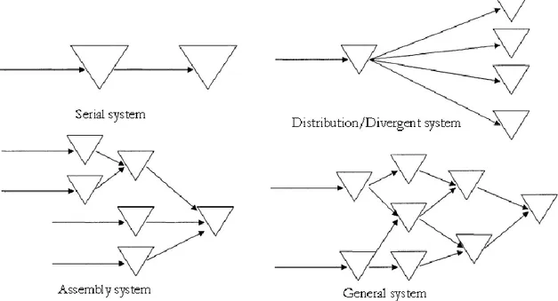
In the serial system each stock has at most one immediate successor and at most one predecessor, see Figure 2.2. For the pure distribution systems each stock point has at most one predecessor but an arbitrary number of successors. A stock point in an assembly system has an arbitrarily number of predecessors but at most one immediate successor. If each stock point can have an arbitrarily number of both predecessors and successors this system is called a general multi-echelon inventory system.
Figure 2.2 Upper left corner: a serial system. Upper right corner: a two-echelon distribution system. Lower left corner: a three-echelon assembly system. Lower right corner: a general multi-echelon
system.
The different types of multi-echelon systems shown in Figure 2.2 are quite different in an inventory control context, and different multi-echelon models are required for controlling and evaluating them. Other characteristics of the inventory system also influence how it can be controlled.
- High / Low demand. Systems with high demand generally require approximate methods, as exact methods tend to be computationally very demanding.
- Repairable / Consumable items. Repairable items needs to be transported upstream in the system.
- Centralized / Decentralized organization. Is each stock point included in single organization so that they can be regulated centrally or are the administrated by a multiple number of independent organizations.
- Lateral transshipments. Items can be transported between parallel stock points in order to avoid shortages.
I will now focus on the two-echelon distribution system, for consumable items. For simplicity, no lateral transhipments will be regarded. For a more detailed introduction of different types of multi-echelon systems and models see, for example, van Houtum et al (1996).
2.2.1. Uncoordinated control of multi-stage inventory systems
As previously mentioned we refer to an uncoordinated approach to control multi-stage inventory systems when single-echelon models are used to control stocks that are in fact connected and interdependent. Each stock point in the system is treated as independent with a set leadtime and service level, optimal reorder points is then determined using a forecast for the demand at this site.
The obvious strength of this method is its simplicity, multi-echelon method are in general much more complex. The weakness is that it does not describe the real system in an adequate way and obvious interdependencies in the system are not taken into account, and as a result suboptimal solutions are produced.
In an uncoordinated approach two problems arise: (1) How we should determine the warehouse demand, this demand is in fact fully determined by the retailer demand and to do an extra forecast introduces an extra layer of error and a risk for bullwhip effect. (2) Since we assume that the purpose of the system is to serve the end-customer, the question is to deploy the safety stock in the system in the most efficient way to achieve this objective
in time. How should then the service level for the warehouse be set? The choice of service level goal at the warehouse will affect the leadtime to the retailer. With a low central inventory, orders from the retailers will often be delayed and, as a result, it may be necessary to increase the retailers reorder points. In an uncoordinated approach the last remark is not taken into account and the resulting solution will thus be suboptimal. 2.3. Coordinated multi-echelon inventory optimization methods 2.3.1. The considered multi-echelon models - preliminaries
The two considered methods deal with approximate optimization of the reorder points for continuous review (R, Q) policies in a two-echelon distribution inventory system. The batch quantities are assumed to be given. The stochastic customer demand occurs at the retailers. It is stationary with known mean and standard deviation, and is independent across retailers and over time. The retailers replenish their stock from the warehouse, and the warehouse in turn places its order with an outside supplier with supposedly infinite stock. Stockouts at both echelons are backordered and delivered on a first-come first-serve basis. All transportation times are constant but the retailer leadtimes are stochastic because of delays due to shortages at the warehouse. Also, to minimize the long run average system costs with respect to reorder points, the investigated methods use a cost structure with linear holding cost and shortage costs.
The following notation will be used for both methods. N number of retailers
li constant transportation time for an order to arrive at retailer i from the warehouse
L0 constant leadtime for an order to arrive at the warehouse from the outside supplier
q largest common factor of Q0, Q1, Q2, …,QN, i.e., q is the largest positive
integer such that all batch quantities are integer multiples of q (q may correspond to a package size or could be 1), this factor is referred to as a subbatch.
Qi batch size at retailer i, expressed in units
Q0 batch size at the warehouse, expressed in units
hi holding cost per unit and time unit at retailer i h0 holding cost per unit and time unit at the warehouse
pi shortage cost per unit and time unit at retailer i;
Ri reorder point for retailer i
R0 warehouse reorder point expressed in units of q
Ci expected cost per time unit at retailer i C0 expected warehouse cost per time unit
C expected total system cost per unit of time
μi(t) mean of the demand at retailer i during time period t
Vari(t) variance of the demand at retailer i during during time period t
μi expected demand per time unit at retailer i
μ0 expected demand per time unit at the warehouse Σi μ i
Vari variance of the demand per time unit at retailer i Var0 variance of the demand per time unit at the warehouse
pi,k(L0) probability for k orders at retailer i during the warehouse leadtime
μiw(L0) average demand from retailer i at the warehouse during the warehouse
leadtime Variw(L
0) variance of the demand from retailer i at the warehouse during the
warehouse leadtime μw(L
0) average demand from the retailers at the warehouse during
the warehouse leadtime = Σi μwi(L0)
Varw(L
0) variance of the demand from the retailers at the warehouse during the
warehouse leadtime = Σi Varwi(L0)
D0(L0) stochastic demand at warehouse during leadtime, expressed in units
2.3.2. Model 1: Heuristic coordination of a decentralized inventory systems using induced backorder costs
Introduction
The choice of a reorder level at the warehouse affects the retailers’ leadtimes, which in turn influences the reorder level decisions at the retailers. To coordinate the control of the inventories in the distribution system this method introduces an induced backorder cost, β, which captures the impact that a reorder level decision at the warehouse has on the
retailers. When an appropriate induced backorder cost is determined it is possible to optimize the reorder level at the warehouse. A relationship between the warehouse reorder level and the retailers’ leadtimes can then be used to provide the lead-time estimate
necessary for optimizing the reorder points at the retailers.
The method builds on the results from three research papers: The first (Andersson et al. 1998) presents an iterative procedure to find an induced backorder that minimizes the expected total system costs, β*. In this paper the stochastic retailer leadtimes are replaced by their averages and all retailers are assumed to use a common batch quantity, Q0. For
general settings the iterative procedure is too computationally demanding in order to be used commercially. The second paper (Andersson et al. 2000) develops the model to allow for retailers to use individual ordering quantities. In the third paper (Berling & Marklund 2006) the iterative procedure in the first paper is used to build an understanding on how the optimal induced backorder cost depends on the parameters of the inventory system. This knowledge is then used to create closed form estimates which produce near-optimal induced backorder costs that will be denoted as β*. An emphasis is placed on large systems with high demand and/or many retailers for which existing methods are not
computationally feasible. The model assumes normally distributed demand and that, in case of shortages, orders are shipped when they can be delivered in full.
The optimization of the reorder level is performed in 6 steps: (1) The warehouse demand is determined (note that this is independent of the retailers’ reorder points). (2) The system parameters are normalized. (3) The near-optimal induced backorder cost, β*, is determined using the normalized system parameters. (4) A single-echelon method is used to determine
the optimal warehouse reorder point. (5) Given the optimized warehouse reorder level the stochastic retailer leadtime is determined and then replaced with its average. (6) Finally, the retailer reorder points can also be determined using ordinary single-echelon methods.
Step 1: Warehouse leadtime demand mean and variance
D0,q(L0) stochastic leadtime demand at the warehouse expressed in units of q
Defining F(x) as the cumulative distribution function (cdf) of the associated gamma distribution (see 2.1.5), we use (2.21) to construct a probability mass function (pmf) to approximate the discrete warehouse lead time demand probabilities, P(D0,q(L0)=u) for
u=0,1,…. ,... 2 , 1 ) 5 . 0 -( -) 5 . 0 ( 0 ) 5 . 0 ( ) ) ( ( 0, 0 u for u F u F u for F u L D P q (2.21)
It is noteworthy that the mean and variance of the constructed pmf may deviate slightly from w(L
0)/q and Varw(L0)/q2.
Step 2: Normalize system parameters
To reduce the number of parameters that need to be varied independently Berling & Marklund (2006) propose that the system can be normalized with respect to li, μi and hi.
This means that a time unit is defined so that li is 1, a unit of demand is defined so that μi is
100, and a monetary unit is defined so that hi is 1. Figure 2.3 shows the relationship between original and normalized system parameters and corresponding β* values. Figure 2.4 provides an illustrative example of how the transformation is performed, when q is 1.
Figure 2.3 Relationship between original and normalized system parameters and corresponding β values (source: Berling & Marklund 2006).
Figure 2.4 Example illustrating the normalization procedure (source: Berling & Marklund 2006).
Step 3: Near-optimal induced backorder cost
The near-optimal induced backorder cost for orders from retailer i is denoted βi* and estimated through (2.22). Table A1 and Table A2 in Appendix A provide tabulated values for g(Qi,n, pi,n) and k(Qi,n, pi,n). If the values of Qi or pi fall outside the tabulated range, use the
estimated closed form expressions for g(Qi,n, pi,n) and k(Qi,n, pi,n) presented in Berling &
Marklund (2006), see also Appendix A.
) , ( , , , , , ) , ( * kQin pin n i n i n i i i h g Q p (2.22)
A single induced warehouse backorder cost is estimated as a weighted average with respect to the average demand rates.
* * 1 0 i N i i
. (2.23)Step 4: Optimal warehouse reorder point
The objective is to find a near optimal reorder point to the original system by minimizing the expected holding and induced backorder costs at the central warehouse, C0(R0).
) R ( C0 0
y u q Q R R y u L D P u y Q q h 0 0 , 0 1 0 0 ) ) ( ( ) ( *) ( 0 0 0 q L Q R q w ) ( 2 1 * 0 0 0 (2.24)It is easy to show that, as >0, C0(R0)-C0(R0-1) is increasing in R0, which implies that )
R (
C0 0 is convex. Thus an optimal R0can therefore be found through a simple search
R :C (R )-C (R -1)≤0
max
R*0 0 0 0 0 0 (2.25)
Step 5: Retailer leadtimes
Eq (2.26)-(2.28) provide an approach to approximate the average retailer leadtime proposed in Andersson & Marklund (2000). Numerical observations have shown that a large retailer in terms of μi and Qi tends to have longer mean leadtime, Li. In other words, a retailer which orders often and in large quantities have, relatively speaking, more units backordered and reserved at the warehouse than a retailer with low ordering frequency and small order quantities. This step is more thoroughly described in Andersson and Marklund (2000) section 5.2.
Define i
L expected lead-time for an order to arrive at retailer i
) (B0
) ( 0r
B
E expected number of reserved subbatches at the warehouse
(ordered by a retailer at the central warehouse but not yet shipped)
0 0 1 E(B )q/
mean delivery delay due to stockouts at the warehouse
0 0
2 E(B )q/
r
mean delivery delay due to reserved units waiting to be shipped
N i i i i Q q 1 ) (
y u 0 q , 0 Q R 1 R y 0 0 q , 0 ) L ( D Q R 1 R y 0 0 (u y)P(D (L ) u) Q 1 ) y ) L ( D ( E Q 1 B E 0 0 0 0 q , 0 0 0 0 (2.26) i i i i i i l q Q N q Q L 1 2 1 1 1 1 ) ( ) / ( ) ( (2.27)Where (x)+ = max(x, 0). The first two terms in (2.27) represent an estimate of the mean
delivery delay to retailer i due to stockouts at the warehouse and reserved units waiting to be shipped respectively. The estimate is found by differentiating the average delivery delay due to stockouts over all retailers based on the relative size of the retailer’s relative
deviation from the average retailer size, measured in terms of the product μi(Qi – Q), as a
basis for estimating the stockout delivery delay to that same retailer. The third term in (2.27) represents an estimate of the mean delivery delay to retailer i due to the existence of reserved units at the warehouse. The last term is the constant transportation time.
To get an explicit expression for ( 0)
r
B
E Andersson & Marklund suggests another
approximation, inspired by an idea in Lee and Moinzadeh (1987). This approximation is based on the observation that reserved units only occur when a fraction of a retailer’s order quantity is backordered. In (2.28) Q can be interpreted as an average batch size. If we divide the number of backordered units B0 by Q and the result is fractional, say 2.45, this
indicates, due to the complete delivery policy at the warehouse, that the total number of delayed units is 3 Q and subsequently that 0.55 Q units are reserved at the warehouse.
Define
x the smallest integer >= x
N i i i Q 1 0 = Demand intensity at the warehouse in number of retailer orders
N i N i i i i i Q Q Q 1 0 1 0 ) ( ) ( 0r 0 Q E Bo Q B E B E (2.28)Step 6: Optimal retailer reorder points
With an estimate in place the retailer reorder points can now be determined in analogy with step 4 by minimizing (2.29) with respect to Ri.
i i i i i i i i i i i i i i Q R H R H Q b h Q R h C 0 2 0( /2 ) ( ) (2.29)
2.3.3. Model 2: Approximate optimization of a two-echelon distribution inventory system
Introduction
The method originates with Axsäter (2003) and is based on normal approximations for both the retailer demand and the demand at the warehouse due to orders from the
retailers. The approximations make it computationally feasible to optimize by successively searching for the set of reorder points that generates the least costs.
In short, the method can be described in six steps: (1) The warehouse demand mean and variance is determined. (2) For each feasible warehouse reorder point, the mean and variance for the retailer leadtime is determined. (3) Optimal retailer reorder levels for each feasible warehouse reorder level are determined and total costs for each solution is
costs. Both warehouse and retailer demand is assumed to follow normal distributions. An excel macro that executes this inventory optimization algorithm can be found at:
http://www.iml.lth.se/Sven/Approximate%20Optimization.xls.
We define
μiLT mean of the stochastic leadtime faced by retailer i
VariLT variance of the stochastic leadtime faced by retailer i
Step 1: Warehouse leadtime demand mean and variance
First, the warehouse leadtime demand mean and variance, μw(L
0) and Varw(L0) is
determined. To do this the probability for k orders at retailer i during the warehouse leadtime, pi,k(L0), is approximated by
dx L L Q k x L L kQ x Q L p Qi i i i i i i i k i
0 0 0 0 0 0 , ) ( ) ( ) 1 ( ) ( ) ( 1 ) ( ) ( ) ( 2 ) ( ) ( ) 1 ( ) ( ) ( ) 1 ( ) ( 0 0 0 0 0 0 0 L L kQ G L L Q k G L L Q k G Q L i i i i i i i i i i i , (2.30)where G(x) is defined by (2.11) in section 2.1.6. Refer to Axsäter (2003) or Andersson et al (1998) for details on how pi,k(L0) is derived. pi,k(L0) is determined for all k for which the
probability is not too low, k is under normal conditions a small number. It follows that
) ( ) (L0 i L0 w i and (2.31)
k k i w i i w i L kQ L p L Var , 0 2 0 0) ( , (2.32)We now fit a normal distribution to the warehouse leadtime demand and determine its mean and variance, μw(L
0) and Varw(L0), by summing μiw(L0) and Variw(L0) over i.
Step 2: Mean and variance for retailer leadtimes
The mean and variance of the leadtime faced by the retailers are modelled as a function of the warehouse reorder point R0, the delay is assumed to be equal for all retailers. Using
Little’s formula the mean leadtime for the retailers are obtained from the expected number of backorders and the total demand,
N i i i LT i I E l 1 0) ( . (2.33)The variance of the retailer leadtime can be expressed as
2 2 ) ( ) ( E VariLT , (2.34)
where δ is the stochastic delay at the warehouse for retailer orders and μδ is its mean. The
mean and variance of the retailer leadtime are calculated for each feasible warehouse reorder point R0. For a complete derivation of these equations, see Axsäter (2003).
Step 3: Optimize retailer reorder levels
A normal distribution is fitted to the retailer leadtime demand and μi(LT) and Vari(LT)
determined through, i LT i i LT ( ) and (2.35) LT i i LT i i i LT Var Var Var( ) ( )2 . (2.36)
Optimal retailer reorder points are calculated for each feasible warehouse reorder point by minimizing the retailer cost function,
( ) ( ) ) , ( 0 i i i i i i R R hE I p E I C . (2.37)
The formulas for the expected number of backorders and the expected stock level, E(Ii)
-and E(Ii)+ are omitted here (again, see Axsäter 2003). We denote the optimal reorder point
for a given R0 by Ri*(R0). Since Ci(R0, Ri) is a convex function in Ri given R0 (see Axsäter
2000) the minimum is found using a computationally fast search procedure over Ri.
Step 4: Optimal warehouse reorder level
In the last step the warehouse costs are calculated for each feasible warehouse reorder point using ( ) ) ( 0 0 0 R h E I C o , (2.38)
where E(I0) is the expected inventory level. Now the optimal warehouse reorder point, R0,
and the corresponding optimal retailer points, Ri*(R
0), are found by minimizing the total
)) ( , ( ) ( ) ( 0 1 * 0 0 0 0 C R C R R R R C N i i i
. (2.39)Too make optimization fast we disregard that C(R0) is not necessarily convex and just look for a local minimum.
3. METHOD OF EVALUATION
This chapter explains how the performances of the optimization methods were investigated and compared. First a simulation model was constructed to represent the inventory system in the testing phase, see Section 3.1. The inventory data was analysed and three base cases selected, see Section 3.2. In-data to the simulation environment was supplied using the inventory data and output (reorder points) from the three optimization models, see Section 3.3. Lastly, the output data from the simulation was analysed to compare the optimization methods, Section 3.4.
3.1. Simulation model
The simulation of the inventory system is performed using a discrete event simulation model in the simulation software Extend. A reason for using a high-level programming software like Extend is that considerable time can be saved in constructing the model. Also, the foundation for the simulation model was already available through another research project (Howard, C. 2007). The logic of a two-echelon inventory system, as described in Section 1.2, was implemented in the simulation model. See Appendix D for more information on the simulation environment.
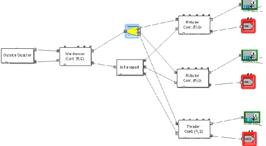
Figure 3.1. Graphical representation of the simulation model.
A graphical representation of the simulation model is presented in Figure 3.1, which is a screen dump from Extend. The rightmost blocks without the arrow generates customer
events with an intensity and order sizes according to a compound Poisson process. As described in Section 2.1.6 this process is often used to model demand data accurately, see this section for a more thorough discussion. The customer event is sent to the connected block labelled “Retailer Cont (R, Q)” which simulates a stock point governed by a
continuous review (R, Q) policy. The ordered items, represented by the customer events, which can be delivered immediately exits to the right entering to the block marked with an arrow, the ordered items that cannot be delivered are backordered. When the inventory position of the stock point reaches its reorder point an order of size Q is generated and sent to the block labelled “Warehouse Cont (R, Q)” which simulates a stock point in the same way as the retailer block. The warehouse block treats incoming orders the same way as the retailer block treats customer events. When an order (or part of an order) from a retailer is fulfilled, a replenishment event is triggered and sent to the “In transport” block, which delays the event for a set amount of time. After the event is delayed it is relayed to the retailer block, where the stock is replenished by the amount of units set by the ordering level of the retailer block. Order events triggered at the warehouse block is sent to the block labelled “Outside supplier”, where the event is delayed for a set amount of time and then sent back to the warehouse where the stock is replenished.
3.2. Selecting test cases
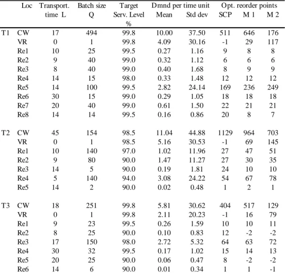
The inventory data supplied by Tetra Pak Technical Service AB in Lund was analysed to find adequate test cases. The data contained information on 80 products, characterized as spare parts, stocked in an inventory system that consisted of one central warehouse and 19 retailers. Few products were stocked at all 19 retailers. For each article and stock point the data included the following information:
- Order quantity
- Transportation time (time to transport unit from supplier to stock point) - Target service level (fill rate)
- Achieved service level (fill rate)
- Date, time and size for orders during a period of three years
Tetra Pak views the distribution system as a part of the value chain and therefore increases the value of an item by 20% when it arrives at a retailer. The inventory data was analysed
statistically to provide an overview, tables and plots from this analysis is provided in Appendix B. An interesting observation is that for most products a large portion of the demand took place directly at the warehouse, a direct upstream demand. Three products were selected to provide in-data for the simulation environment, for a specification see Table 4.1 in Section 4.1, these items will be referred to as the base cases. The rationale behind this selection was primarily the fact that it’s only relevant to evaluate the multi-echelon models in conditions they are designed for. We know that, in their current form, the methods are not designed for situations where the direct upstream demand is large or the total system demand low; in those cases other methods should be used. Therefore, only products where the total demand was more than five units/day and where the direct upstream demand comprised less than 60% of the total demand was considered. Within these limits the three products was selected to cover as much of the diversity in total inventory system demand, number of retailers, total system demand and mean size of the customer orders. All 80 products are plotted with respect to total demand and percentage of direct upstream demand in Appendix B.
3.3. Supply in-data for the simulation
The following parameters are needed to provide in-data to the simulation model: - Transportation times from the outside supplier to the warehouse and from the
warehouse to each retailer.
- Holding costs at all locations and shortage costs at all retailers. - Ordering quantities for the warehouse and the retailers.
- Parameters for the compound Poisson process that generates the retailer demand. - Reorder levels at the warehouse and each retailer.
The transportation times are readily available in the supplied inventory data and can be used directly. The need for holding costs and shortage costs arise since Method 1 and 2 are both, in their current form, so called backorder cost models. Since we are only interested in the relative performance of the optimization models, the retailer holding cost is normalized to 1 and, to accommodate for the fact that the value of the an item increases 20% when it reach the retailer, the warehouse holding cost is set to 0.84.
The shortage cost was derived from the target service level, that is available in the supplied inventory data, according to the process discussed in Section 2.1.6, Eq. (2.18) and (2.19). As noted in this section this method only produces accurate results for the fill rate when the demand is continuous or generated by a pure Poisson process. As the demand is generated by a compound Poisson process in the simulation model, the translation process will only be accurate when the service level is measured as a ready rate. This means that Method 1 and Method 2 is in fact optimizing the reorder level with regard to the ready rate (in the inventory data both the target and the achieved service level is measured with the fill rate in mind). Since the same is true for the uncoordinated method, as it assumes continuous demand, this does not constitute a problem when comparing the coordinated optimization models of the backorder type with the uncoordinated method which uses a service level constraint. However, there is an underlying problem of misalignment between the target service level and the service level used in the optimization of the reorder points for both the conventional single-echelon method and the investigated multi-echelon models.
Even though a parameter for the order quantity was explicitly available in the inventory data this value was not used when defining the test cases. The analysis of the inventory data showed that the actual size of the replenishment orders from the retailers did not follow the set order sizes. As the model assumes fixed order quantities the average of all replenishment orders from a retailer was used when defining the order quantities actually used in the test cases. The alternative, to fit the order quantities from the inventory data to a distribution and then treat them stochastically in the simulation model was disregarded for sake of simplicity. For the warehouse, the order quantity parameter available in the inventory data is used without modification since there is no data for the order placed with the outside supplier.
The arrival rate for the compound Poisson process that generates the retailer demand is determined as the mean number of customers arriving each day. The assumption of exponentially distributed interarrival times and gamma distributed customer order sizes was validated by series of goodness-of-fit tests; Kolmogorov-Smirnov test, Anderson-Darling test and Cramér-von Mises test. For a thorough discussion of these tests, see
D'Agostino and Stephens (1986). A discrete gamma distribution is fitted to the mean and variation of the customer order sizes and used as the compounding distribution. The gamma distribution was chosen because both its mean and variance can be varied through its parameters, it is non-negative, and it proved a good fit with the data. Arrival intensity, customer order sizes and demand data for the three test cases together with the resulting demand parameters is presented in Appendix C.
3.3.1. Virtual retailer
As mention in section 3.2, a common feature in the analysed test data was that a large portion of the customer demand takes place directly at the warehouse. This is sometimes called direct upstream demand in the literature. The evaluated models for coordinated control are not specifically constructed to handle this. The way around this dilemma is to model the direct upstream demand as a separate retailer, a virtual retailer that is a separate stock reserved for direct customer demand at the warehouse (see Axsäter 2007). The order quantity for the virtual retailer is always 1 and the leadtime is set to 0. For the
uncoordinated approach the reorder level is always set to -1. This means that each customer demand at the virtual retailer triggers a corresponding warehouse order of the same size. There will never be any stock on hand at the virtual retailer in the uncoordinated case. This is generally not true for a coordinated approach; in this case a reorder level is determined in the same way as for the other retailers.
3.3.2. Calculate reorder levels
The last step when defining the test cases is to determine a set of reorder levels for each of the evaluated optimization methods. Reorder levels are calculated for Method 1 and Method 2 using software provided by Johan Marklund and Sven Axsäter respectively. For the uncoordinated method, the SCP method, the order levels were calculated using documentation received from the ERP company that initiated this project.
The simulated warehouse mean and variance is used as input when determining reorder levels for the SCP Method. In real conditions, an extra forecast with accompanied forecast error would have to be made at the warehouse. As this extra layer of error is eliminated by providing the method with an exact value for the warehouse demand this provides a slight