«L å ,; . . g I f }
$
$
.m
mm
f
r
å
m
=>
VTI särtryck 298 - 1998
Tinbergen Revisited
Benefits from Infrastructure Investments
in an Open Economy
Imdad Hussain, VTI and
Lars Westin, Umeå University
Swsdisii
Rami and
TINBERGEN REVISITED: BENEFITS FROM
INFRASTRUCTURE INVESTMENTS IN AN
OPEN ECONOMY
Imdad Hussain & Lars Westin
Umeå Economic Studies No. 431
,
UMEÅ UNIVERSITY 1997
Tinbergen Revisited: Bene ts from Infrastructure
Investments in an Open Economyl
Imdad Hussain
Swedish Road and Transport Research Institute (VTI) S-981 95 Linköping
Lars Westin
Department ofEconomics
Umeå University
S-901 87 Umeå
SwedenLars.Westin @ natek.umu.se
November 1996 ABSTRACTIn his seminal work, Tinbergen (1957) studied the impact of an infrastructure
improve-ment on the transport cost of existing traffic and on the national product. In a numerical
example it was shown that the national product could increase substantially beyond the
value of the reduced cost of transportation on the improved link. This di erence has been labelled the Tinbergen multiplier. Since the modelled economy was thought of as a
rst best case, the result has been used among those arguing that transport investments
give rise to substantial Spill over effects in the economy. However, the result is in
contra-diction with later results within multimarket welfare analysis under rst best assumptions.
In this paper we recalculate Tinbergen s model and show that the spectacular result is
heavily dependent on the localisation of the transport sector. Hence, our results are of
utter importance for today s models of infrastructure assessment.
JEL Classi cation: D61, R13, R42
Keywords: Infrastructure investments, spatial cost-bene t analysis, multimarket welfare analysis, Tinbergen multiplier.
1 Financial support has been received from the Swedish Transport and Communications Research
1 Introduction
Tinbergen (1957) was probably the rst attempt to consider a transport investment
appraisal in a spatial economy-wide numerical framework. In his seminal paper, a road
construction scheme is evaluated by measuring transport cost savings for existing tra ic as well as the national product change at initial prices. The main conclusion is that transport cost savings for existing traf c substantially underestimate the economy-wide bene ts of the road investment. The result is frequently referred to and discussed in studies of transport investment appraisal. Often cited are also Bos and Koyck (1962) or
Liew and Liew (1985) which have reported similar results using models with a similar
basic structure. However, the result by Tinbergen is noticeably different from those
achieved by Lesourne (1975), Dodgson (1973), Jara-Diaz (1986), or Kanemoto and Mera (1985). The message in the latter studies is that in a rst best economy, bene ts to
existing and new traf c on the improved road represent total bene ts in the economy.
Since independent of this, the result by Tinbergen seems to attract politicians and the common debate it is of interest to revisit and explore the structural properties of the model by Tinbergen deeper.
A rst observation is that Tinbergen measured bene ts to tra ic as transport cost savings
for existing traf c. A part of the discrepancy may for this reason be explained by bene ts to newly generated traf c. However, new traffic alone may not explain the large difference suggested by what has been known as the Tinbergen multiplier. Obviously, the model must contain subtle assumptions which contradict the results established in modern welfare theory.
In this paper, the structure of the Tinbergen model is presented in line with the spatial computable general equilibrium tradition while the speci cation of the transport sector as
an imported good is shown to be critical for the result in the original paper. We then let
the transport sector become a domestic part of the economy and recalculate the
measures of bene ts. It is found that the revised model produces results which are
compatible with the contemporary general equilibrium welfare theory. The general lesson
of importance for current applications is that the size of the Tinbergen multiplier is
critically dependent on the spatial origin of the transport sector and the net of the balance of trade. Hence, while Tinbergen was right in case the economy is Open but not by assumption in external balance, the result is not valid for a closed economy. Nowadays, when cost-bene t analyses are made on regions and nations which may by no means be
treated as closed or in external equilibrium, this distinction between closed and open
economy CBA becomes even more important. The result is in line with comments on the need for open economy cost-bene t analysis already made by Mohring, 1993.
2
Tinbergen s three region model
Tinbergen develops a simple model consisting of three regions producing four
commodities. Commodity one, two, and three are respectively produced by regions one, two, and three while commodity four is produced both by region two and three. Demand is in the latter case characterised by a spatially in nite elasticity of substitution implying that consumers buy from the cheapest region. No taxes, transfers, savings or investment costs are considered explicitly. Neither are explicit demand and supply mctions for primary factors considered, a simpli cation not critical for the results.
The demand price in region j of commodity h produced in region r, pg , is in Tinbergens paper given by Pqu , which equals the factory gate price multiplied by the transport cost factor between region r and j. Given this, the unit transport cost of carrying commodity h
from region r to region j is pf tg = pf (Trj 1) where tg represents the unit transport cost
coe cient between the two regions. The demand price pg. may then also be expressed as
pf (1 + tg) . Since the unit transport cost coefficient between region r and j by Tinbergen was assumed to be independent of the good transported, we may use tn instead of tg- in the sequel.
Deliveries of commodity h produced by region j to region r are denoted vga. Those deliveries give revenues in the region of origin j, yj, which include the transport cost paid by other regions. Thus, for each region we have the following revenues or incomes,
y,(p,v)=§§p§'(1+t,-,)vt=>h:§p§ vt+.§:>;p?t,-,v;
Vi
(1)
In the last part of the equation, the rst term gives receipts net of transport costs while the second term represents the transport costs paid by other regions on goods produced
by region j. Vectors of prices and delivered quantities are denoted by p and v
respectively. Given regional incomes, the price and income dependent demand Emotion
in region j for commodity h produced in region r may be formulated as,
h
(py-(pw)
d?- ,
J(P Y)=
Ph(1+tq)J
l ;O<(pg<l and ZZcpgzl Vr,h,j (2) h rIn the equation, (på is the share of incomes in regionj spent on commodity h produced in region r. This demand function is also conditional upon the following constraints,
(i) d3>o
if
pig=min{p:;}
van
(ii) (it;-=O if
pigmnwg}.
vf,h,j
The above conditions are in the model by Tinbergen applicable to commodity four, which is produced by both region two and three. The aggregate supply function of region j for commodity h is dependent on available capacity and the relative mice compared to
other commodities,
Above, v? is the supply of commodity h in region j while 'o'-ål represents the capacity limit for this commodity. The symbol o? determines the supply elasticity of the function. The interpretation of the supply function is that a decrease in the price of a commodity ceteris paribus reduces supply. Since investments in production capacity is absent in the model, a region without a positive initial capacity will not produce a commodity after the
improvement. Given the above conditions of supply and demand, the market equilibrium
is ensured by equations (4) and (5) below.
erdir(P,Y)=§vir(P)=v§ (P)
vm.
(4)
Zn (RV) = Y
(5)
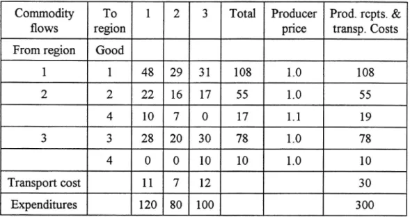
Equation (4) secures that total supply of each good equals total demand in the economy while (5) implies that regional incomes or expenditures including transport costs, aggregated across all regions equals the exogenously given national income Y. Equations (4) and (5) represent a system of six equations in ve endogenously determined equilibrium prices. One of the equations becomes redundant due to Walras Law. Since the aggregate national product was xed by Tinbergen at 300 units it thus acts as a numeraire and a system of ve equations and ve variables is obtained. Basically, the data used in Tinbergen s model consist of interregional ows, initial and new transport cost coef cients and parameters of the supply and demand functions. In table l below, the initial equilibrium according to the original model is shown.
In the table, interregional commodity ows, total supply, producer prices and transport
costs paid by each region are given. Although the total transport cost paid by all regions
by de nition must equal total receipts of transport revenues in the economy, the
transport costs paid by an individual region do not have to equal its receipts of transport
revenues from other regions.
Table 1 Commodity ows, incomes, receipts and transport costs in the initial equilibrium. Data from Tinbergen (1957).
Commodity
To
1
2
3
Total Producer Prod. rcpts. &
ows region price transp. Costs From region Good
1
1
48
29
31
108
1.0
108
2
2
22
16
17
55
1.0
55
4
10
7
0
17
1.1
19
3
3
28
20
30
78
1.0
78
4
0
0
10
10
1.0
10
Transport cost 11 7 12 30 Expenditures 120 80 100 300Transport costs paid by each region are also shown and aggregated to total receipts of transport revenues in the economy. The last column and row of the table show
producers receipts from the sale of commodities and expenditures by each region
respectively. It follows that the income in each region is fully spent on goods and the
transport costs involved to obtain the goods.
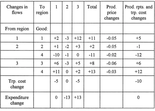
In his comparative static equilibrium analysis, Tinbergen assumed that a transport
improvement between region one and three is made. Table 2 gives the changes in
interregional commodity ows, producer receipts, producer prices and transport costs brought about by this sixty-six per cent reduction in the unit transport cost coef cients. In the new equilibrium, region one demands commodity four from region three instead of region two since the reduced transport cost made region three the cheapest supplier of the commodity. As expected, all producer prices have decreased while the supply of each
good has increased. The table also shows that the overall change in producer receipts
including those occurred in transport sector revenues sum up to zero. This property is due to equation (5) which keeps the national product at the given level.
Table 2
Impacts of a sixty-six per cent reduction in the transport coef cient
between region one and three. Data from Tinbergen (1957).
Changes in
To
1
2
3
Total
Prod.
Prod. rpts. and
ows region price trp. cost changes changes From region Good:
1 1 +2 -3 +12 +11 0.05 +5 2 2 +1 -2 +3 +2 -0.05 -1 4 -10 -1 O -11 -0.02 -12 3 3 +6 -3 +5 +8 -0.06 +6 4 +11 0 +2 +13 -0.03 +12 Trp. cost -5 O -5 -10 change Expenditure 0 -13 +13 0 change
3
Bene t measures in Tinbergen s model
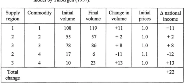
Given the two sets of equilibria above, welfare impacts of the improvement may be calculated. The economy-wide bene ts were by Tinbergen measured as the increase in
national product at initial prices, while the bene ts to traf c were calculated as transport
cost savings for the existing traf c ow on the improved road. Using the symbols ° and 1 indicating initial and post-improvement values respectively, the change in the national product is,
A? = zzng°vgl zzng°vg°
j r h j r h(6)
The above measure is computed as the change in demand for each product evaluated at initial prices including cost of transportation. By aggregating these changes across
regions and commodities, total economy-wide bene ts are obtained. As shown at the bottom of table 3, this increase in national product amounts to twenty two units.
Table 3 Increases in national income computed at initial prices in the original model by Tinbergen (1957).
Supply Commodity Initial Final Change in Initial A national region volume volume volume prices income
1
1
108
1 19
+1 1
1.0
+1 1
2
2
55
57
+ 2
1.0
+ 2
3
3
78
86
+ 8
1.0
+ 8
2
4
17
6
-1 1
1.1
-12
3
4
10
23
+13
1.0
+13
Total +22 changeTransport cost savings for existing tra c are calculated as the product of the unit transport cost reduction and the initial traf c ow in both directions on the road. Bene ts to initial traf c are denoted by BE and calculated as,
BE = Am13 X vi; + Am31 X Vä; . (7)
In (7), the change in unit transport cost is denoted by Am13 and Am31, while the initial
ow of goods in both directions are represented by Vis and vå]. Also, by de nition,
Am13 : PF x (T?3 Tåg) and Am,, : På x (T;1 Tål) , the change in transport cost factors multiplied by initial supply prices give the change in unit transport cost. Observe that the
difference between the initial and post-investment transport cost factors (T; - Ti,-) is
equivalent to the difference between the corresponding initial and post-investment
transport cost coef cients (t;- tå) Table 1 above gives us vi; : 31 and v3: = 28. From
the data on transport costs between regions one and three in the two transport coe icient matrices, the transport cost savings for existing traf c become,
BE = 1.0 x (1.3 1.1) x 31 +10 x (1.3 -1.1) x 28 = 11.8
(8)
In order to obtain a measure of the difference between the economy-wide bene ts and
the transport cost savings for existing traf c ows, the Tinbergen multiplier may be
interpreted as the ratio A? / BE. With the information in table 3 and equation (8), this
multiplier becomes 22/11.8 = 1.9. Having obtained this result, Tinbergen concluded that transport cost savings for existing traf c substantially underestimate economy-wide
bene ts of the investment.
It is now important to point at the assumption so crucial for the conclusions reached by
Tinbergen. Equation (5) above reveals that total output in the economy is absorbed by nal consumption. Since total expenditures on consumption are gross of transport costs,
a part of the national product is devoted to the transport sector. This is evident from
equation (9) below,
y r .
pj 2va = 2
r
) h
)
(:> y; = p?(v£*r + v it i)
V h,]
(9)
In the original formulation by Tinbergen (in the left part of the equation), y; represents
total expenditures by region r on consumption of commodity h produced in region j, including cost of transportation. To the right it is clear that this, as was indicated in (1) consists of both revenues to the delivering sector and to the transport sector. However, in the equilibrium condition (4) only the rst part contributes to the domestic demand for commodities. The transport cost in this way becomes a transfer of revenues abroad
with the implication that transport services are imported from an external transport
agent. Since imports of transport services are not balanced against exports of goods produced in the economy the reduced cost of transportation has a similar function as an
injection to the economy. As will be clear below and as would be expected from general
equilibrium welfare theory, this transfer has important repercussions on the bene t measures in Tinbergen s model.
4
A Tinbergen model with a domestic transport sector
If, contrary to Tinbergens original approach, the transport sector is specified as an endogenous part of the model it will compete with nal demand about the resources in the economy. A reduction in the transport costs will then not act as a net transfer from abroad but as a resource saving investment. This will change both the outcome of the initial and post investment equilibria.
We incorporate this new condition in the model by a change in the equilibrium condition
(4). We assume the transport sector as only input demands an amount of the transported
good as given by (9). Due to this total demand for good j in the economy will change such that the new equilibrium condition becomes,
2 då?, (P, Y) + % t; VHF) = %våi (P) + 2; i; v1}: (P) = v? (P) V haj (10)
The new term is the demand for resources by the transport sector which adds to the
demand for nal consumption. The difference between (4) and (10) is the important aspect of the transport service provision which makes Tinbergen s model a model of an
open economy. In the following, Tinbergen s model will be revised by treating transport
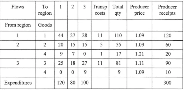
costs according to the formulation above. As one would expect, the new condition changes both the initial and post-improvement equilibrium prices and quantities. The
initial equilibrium in the revised model is shown in table 4 below.
Comparing the initial equilibrium produced by the revised model with the solution in table 1 shows that demand for goods [net of the transport related demand for goods] has decreased in the revised model. The new treatment of the transport sector implies that total output is now absorbed by nal demand as well as by the transport sector. Subsequently, an increase in prices and output is realised as a re ection of the usual
general equilibrium effect.
Table 4 Commodity ows, incomes, receipts and transport sector demand in the revised model. The initial equilibrium.
Flows To 1 2 3 Transp Total Producer Producer region costs qty price receipts From region Goods
1 1 44 27 28 11 110 1.09 120 2 2 20 15 1 5 5 55 1 .09 60 4 9 7 0 1 1 7 1 .21 20 3 3 25 1 8 27 1 1 81 1 . 1 1 90 4 0 O 9 9 1 .09 1 0 Expenditures 120 80 100
3 00 As in the original Tinbergen paper we may now compute the corresponding post-investment equilibrium obtained from the same reduction in the transport cost coef cients. Post-improvement prices and interregional ows are shown in table 5 below.
Table 5 Post-improvement equilibrium according to the revised model.
Flows To 1 2 3 Transp Total Producer Producer region dem. qty. price receipts From region Good
1 1 47 24 40 7 1 1 8 1 .02 1 20 2 2 21 12 18 6 57 1.05 60 4 0 6 0 0 6 1.12 7 3 3 31 16 32 6 85 1.06 90 4 10 0 10 2 22 1.05 23 Expenditures 120 67
1 13
300 12
We may observe that the overall output has increased while equilibrium prices have decreased due to the reduced transport costs. Furthermore, demand for goods in regions
located on the improved road [region one and three] has increased, while it has
decreased in region two. With this new allocation of resources, bene ts of the road investment may be computed.
5
Calculating the Tinbergen multiplier in the revised model
With the data in tables 4 and 5 we may recalculate the two measures of investment bene ts. First, we compute the national income change according to table 6 below. Then we measure transport cost savings for initial tra ic. However we will also calculate the bene ts associated with newly generated traf c on the road, the bene ts which were not
explicitly taken into account by Tinbergen.
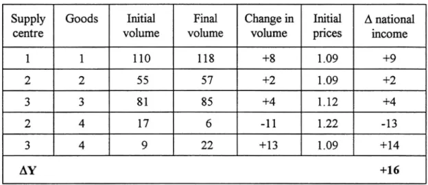
Table 6
The increase of national product at initial prices, with a domestic transport
sector.
Supply Goods Initial Final Change in Initial A national centre volume volume volume prices income
1
1
110
118
+8
1.09
+9
2
2
55
57
+2
1.09
+2
3
3
81
85
+4
1.12
+4
2
4
17
6
-1 1
1.22
-13
3
4
9
22
+13
1.09
+14
AY
+16
Already in table 6 one may observe that the rise in national product computed by the
revised model is less, 16 units, as compared with the 22 units given by the original
model. In order to investigate how this difference affects the size of the bene t multiplier
the transport cost savings for initial traf c are computed. From (7) and (8) we have, 12
BE* = 1.09 x (1.3 1.1) x 28 +112 x (1.3 1.1) x 25 = 11.7
(11)
A comparison between (8) and (11) indicates that the two versions of the model lead to almost exactly the same measure of bene ts in terms of transport cost savings for existing traf c. Given this, we may summarise the above results by comparing the
Tinbergen multiplier (TM) produced by the two cases:
A?
22
TM ori inal = = z1.9 12( g ) BE 11.8
( )
A?
16
TM revised = z zl. 13(
)
BE" 11.7
( )
The difference between the above multipliers show that the extent to which transport cost savings for existing traffic underestimate the increase in national income is much less
in the case with a domestic transport sector. Nevertheless, a considerable discrepancy
between the economy-wide bene ts and the transport cost savings for existing traf c
remains.
As mentioned, Tinbergen did not take into account the welfare gains associated with
newly generated traf c. Bene ts to generated tra ic may be captured by considering changes in the interregional commodity ows, Avg- , on the improved road. Those may be determined as the difference between the initial and post improvement ows between regions one and three provided by tables 4 and 5. For traf c in each direction on the road we obtain,
AVi3ZVii_Vi; =40~28 = 12 (14)
Avglzvgi-v§;=31-25=6.
(15)
Moreover, after the improvement region one buys good four from region three
[vg1 = 10], instead of its initial import of the good from region two [vg] = 9]. This shift
of demand for good four gives a further increase in traf c on the route between regions one and three. For the sake of computational ease we assume, perhaps without much loss of accuracy, that the transport demand segment between the initial and post-improvement situations in these cases is linear. Given this along with (12), (14) and (15) above, the bene ts associated with increased traf c on the improved road may be approximated by using the rule of a half ,
BN<L3>= 0.5 x [1.09 x (1.3 1.1) x12 + 1.12 x (1.3 1.1) x 6] = 1.98 = 2.
(16)
Equation (16) shows the bene ts associated with newly generated traf c from transportation of good one and good three on the improved road. In addition, the gain due to increased tra ic caused by the shift of region one s demand for good four 'om
region two to region three, must also be taken into account. This is denoted by EN )
and measured by the area under the post-investment demand curve for good four by region one. We have,
BN(4)=O-5 X[t§1 tål] X P;; x AVgi +611 X på; X Avgl
(17)
Ol
BW) = 0.5 x [0.3 0.1] x 1.094 x 10 + 0.1 x 1.094 x 10 = 2.2
(18)
By adding BM ) and EN ) total bene ts associated with increased traf c on the
improved road are obtained as,
BN = BN<L3> + BN(4> = 2 + 2.2 = 4.2.
(19)
Given the transport cost savings for existing traf c in (11) and the bene ts to generated traf c in (19), the full bene ts to traf c are measured as,
BT = BE*+BN= 11.7 +4.2 = 15.9 % 16. (20) Apparently, total bene ts to traf c in (20) are almost exactly equal to the national product increase computed by the revised model in table 6. These two bene t measures
give a modi ed Tinbergen Multiplier equal to 16 / 15.9 = 1.006, which is what should be
expected in a model of a rst-best economy. 6 Final comments
In Tinbergen s original model, the reduced transport costs may be viewed as a transfer
from abroad or a reduced tax, which acts as an injection into the domestic economy.
When this injection was removed the economy-wide bene ts decreased and parity with tra ic bene ts was obtained. With this results at hand, we may conclude that in a
rst-best economy, the bene ts of a transport infrastructure investment may always be
captured by considering existing and generated traf c on the improved infrastructure,
provided that provision of transportation services not implies a net transfer of income
from abroad. However, the example also shows that in a regional evaluation of
infrastructure investments, the impact of interregional transfers has to be evaluated and
that the open economy cost bene t analysis has an important relevance in the case of
infrastructure evaluation.
References
Bos, H.C. and M. Koyck (1961) The Appraisal ofRoad Construction Projects - A
Practical Example, Review ofEconomics and Statistics, No.1, pp 13-20. Dodgson, J.S. (1973) External Effects and Secondary Bene ts in Road Investment
Appraisal, Journal of Transport Economics and Policy, pp. 169-185. Dodgson, J.S. (1974) Motorway Investment, Industrial Transport Costs and
Sub-Regional Growth: A Case Study of the M62, Sub-Regional Studies, Vol. 8, pp. 75-90.
Dodgson, J.S. (1984) The Economic Assessment ofRoad Improvement Schemes, Road Research Technical Paper No. 75, HMSO, London.
Friedlaender, A.F. (1965) The Inter-State Highway System, North Holland, Amsterdam.
Harberger, A.C. (1971) Three Basic Postulates for Applied Welfare Analysis:
Interpretive Essay. Journal ofEconomic Literature 9, pp. 485-503.
Hussain, I. (1990) Road Investment Bene ts Over and Above Transport Cost Savings
and Gains to Newly Generated Traf c. Proceedings ofSeminar J Held at the
PTRC. Transport and Planning Summer Annual Meeting, University of Sussex,
England.
Hussain, I. (1993) Comparison of Partial and General Equilibrium Analysis of Bene ts
From Road Improvement. Proceedings of The Fourth CGE Modelling
Conference, University of Waterloo, Ontario, Canada.
Hussain, I. (1996) Bene ts of transport Infrastructure Investments. A Spatial Computable General Equilibrium Approach. Ph.D. diss. Umeå University: Umeå Economic Studies, no 409.
Jara-Diaz, S.R. and Friesz, TL. (1982): Measuring the Bene ts Derived from A Transportation Investment. Transportation Research, Vol. 16B, no. 1, pp.
57-77.
Jara Diaz, S.R. (1986) On the Relation Between Users Bene ts and the Economic Effects of Transportation Activities. Journal ofRegional Science, vol. 26, no 2, pp 379-391.
Kanemoto, Y. and Mera, K. (1985) General equilibrium Analysis of the Bene ts of Large Transportation Improvements, Regional Science and Urban Economics,
15, pp. 343-363
Lesoume, J. (1975) Cost-Bene t Analysis and Economic Theory. North-Holland, Amsterdam.
Liew, OK. and C.L. Liew (1985) Measuring the Development Impact of A
Transportation System - A Simpli ed Approach. Journal ofRegional Science
25, pp. 241-258.
Mohring, H. (1993) Maximizing, Measuring, and not Double Counting Transportation
Improvement Bene ts: A Primer on Closed-and-Open-Economy Cost-Bene t Analysis. Transportation Research Board, Vol. 27B, No. 6, pp. 413-424. Tinbergen, J. (1957) The Appraisal of Road Construction: Two Calculation Schemes.
The Review ofEconomics and Statistics, No. 3, pp. 241-249.
UMEÅ ECONOMIC STUDIES
(Studier i nationalekonomi)
All the publications can be ordered from Department of Economics, University of Umeå, S 901 87 Umeå, Sweden.
Umeå Economic Studies was initiated in 1972. For a complete list, see Umeå Economic Studies No 366 and earlier.
367 368 369 370 371 372 373 374 375 376 377 378 379
Zhang, Wei-Bin: Growth with Renewable Resources, 1995.
Zhang, Wei-Bin: Economic Dynamics with Livestock, 1995.
Zhang, Wei-Bin: An Agricultural Equilibrium Model with Two Groups, 1995. Aronsson, Thomas and Wikström, Magnus: Local Public Expenditures in Sweden.
A Model where the Median Voter is not Necessarily Decisive, 1995.
Aronsson, Thomas, Johansson, Per-Olov and Löfgren, Karl-Gustaf: Investment
Decisions, Future Consumption and Sustainability under Optimal Growth, 1995.
Hultkrantz, Lars: Dynamic Price Response of Inbound Tourism Guest-Nights in Sweden, 1995.
Brännäs, Kurt and Johansson, Per: Panel Data Regression for Counts, 1995. Berglund, Elisabet and Brännäs, Kurt: Entry and Exit of Plants: A Study Based on
Swedish Panel Count Data, 1995 .
Brännäs, Kurt and Karlsson, Niklas: Endogeneity Testing in Micro-Econometric Models, 1995.
Aronsson, Thomas, Johansson, Per-Olov and Löfgren, Karl-Gustaf: On the Proper
Treatment of Defensive Expenditures in Green NNP Measures, 1995.
Westerlund, Olle: Employment Opportunities, Wages and Interregional Migration
in Sweden 1970-1989, 1995.
Axelsson, Roger and Westerlund, Olle: A Panel Study of Migration, Household Real Earnings and Self-Selection, 1995.
Westerlund, Olle: Economic Influences on Migration in Sweden, 1995. PhD thesis.
380 381 382 383 384 385 386 387 388 389 390 391 392 393 394 395
Aronsson, Thomas, Brännlund, Runar and Wikström Magnus: Wage Determination under Nonlinear Taxes - Estimation and an Application to Panel Data, 1995.
Brännäs, Kurt: Explanatory Variables in the AR(1) Count Data Model, 1995. Norén, Ronny: Industrial Transformation in the Open Economy - A Multisectoral
View, 1995.
Brännäs, Kurt and Ohlsson, Henry: Asymmetric Cycles and Temporal Aggregation, 1995.
Brännlund, Runar, Chung, Yangho, Päre, Rolf and Grosskopf, Shawna: Emissions
Trading and Pro tability: The Swedish Pulp and Paper Industry, 1995.
Nordström, Jonas: Tourism Satellite Account for Sweden 1992 1993, 1995.
Brännlund, Runar, Löfgren, Karl-Gustaf and Sjöstedt, Sara: Forecasting Prices of
Paper Products: Focusing on the Relation Between Autocorrelation Structure and Economic Theory, 1995.
Qstbye, Stein: Real Options, Wage Bargaining, Regional Subsidies and Employment, 1995.
Qstbye, Stein: A Real Options Approach to Investment in Factor Demand Models, 1995.
Bergman, Mats A.: Price Competition under Capacity Constraint with Endogenous Timing of Entry, 1995.
Vredin, Maria: Values of the African Elephant in Relation to Conservation and
Exploitation, 1995.
Bergman, Mats A.: Antitrust, Marketing Cooperatives and Market Power, 1995. Brännäs, Kurt and Karlsson, Niklas: Estimating the Perceived Tax Scale within a
Labor Supply Model, 1995.
Sjögren, Tomas and Brännäs, Kurt: Recreation Travel Time Conditional on Labour Supply, Work Travel Time and Income, 1995
Löfgren, Karl-Gustaf, Nordström, Anna and Nyman, Pär: Willingness to Pay for Work Programs for Disabled Workers, 1995
Backlund, Kenneth, Kriström, Bengt, Löfgren, Karl Gustaf and Polbring, Eva: Global Warming and Dynamic Cost-Bene t Analysis Under Uncertainty: An Economic Analysis of Forest Carbon Sequestration, 1995
396 397 398 399 400 401 402 403
404
405 406 407 408 409 410 411 412 413Mortazavi, Reza: Three Papers on the Economics of Recreation, Tourism and Property Rights, 1995. PhLic thesis
Qstbye, Stein: Regional Labour and Capital Subsidies, 1995. PhD thesis
Bask, Mikael: Dimensions and Lyapunov Exponents from Exchange Rate Series, 1995
Aronsson, Thomas, Backlund, Kenneth and Löfgren, Karl-Gustaf: Nuclear Power,
Extemalities and Non-Standard Pigouvian Taxes: A Dynamic Analysis under
Uncertainty, 1996
Johansson, Per and Brännäs, Kurt: A Household Model for Work Absence, 1996
Löfström, Åsa: Arbetsvärdering i akademin. Hur lönestrukturen kan påverkas i ett
företag som arbetsvärderat, 1996
Zhang, Wei Bin: Knowledge, Infrastructures and Economic Structure, 1996 Zhang, Wei-Bin: Economic Growth, Housing and Residential Location, 1996
Zhang, Wei-Bin: Taste Change, Economic Growth and Structural Transformation, 1996
Brännäs, Kurt, de Gooijer, Jan and Teräsvirta, Timo: Testing Linearity against Nonlinear Moving Average Models, 1996
Bergman, Mats A: Estimating Investment Adjustment Costs and Capital Depreciation Rates from the Production Function, 1996
Löfström, Åsa: Variation in Female Activity and Employment Patterns: The case of Sweden, 1996
Zhang, Wei-Bin: Knowledge and value - Economic Structures with Time and
Space, 1996.
Hussain-Shahid, Irndad: Benefits of Transport Infrastructure Investments: A Spatial Computable General Equilibrium Approach, 1996. PhD thesis.
Eriksson, Maria: Selektion till arbetsmarknadsutbildning, 1996. PhLic thesis.
Karlsson, Niklas: Testing for Normality in Censored Regressions, 1996
Karlsson, Niklas: Testing for Exponential and Weibull Distributions in Censored Duration Models, 1996
Karlsson, Niklas: Testing and Estimation in Labour Supply and Duration Models, 1996. PhD thesis.
414
415 416 417 418 419 420 421 422 423424
425 426 427 428 429 430Weitzman, Martin L. and Löfgren, Karl-Gustaf: On the Welfare Signi cance of
Green Accounting as Taught by Parable, 1996
Aronsson, Thomas and Löfgren, Karl-Gustaf: An Almost Practical Step towards Green Accounting?, 1996
Löfström, Åsa: Can Job Evaluation Improve Women s Wages?, 1996
Axelsson, Roger, Brännäs, Kurt och Löfgren, Karl-Gustaf:
Arbetsmarknads-utbildning och utförsäkringsgarantin, 1996
Axelsson, Roger, Brännäs, Kurt och Löfgren, Karl-Gustaf: Arbetsmarknadspolitik,
arbetslöshet och arbetslöshetstider under 1990-talets lågkonjunktur, 1996 Li, Chuan Zhong: Semiparametric Estimation of the Binary Choice Model for
Contingent Valuation, 1996
Li, Chuan-Zhong, Löfgren, Karl-Gustaf and Hanemann, W. Michael: Real Versus
Hypothetical Willingness to Accept. The Bishop and Heberlein Model
Revisited, 1996
Li, Chuan-Zhong and Löfgren, Karl-Gustaf: Renewable Resources and Economic
Sustainability. A Dynamic Analysis with Heterogeneous Time Preferences, 1996
Cameron, A. Colin and Johansson, Per: Count Data Regression using Series
Expansions: with Applications, 1996
Brännäs, Kurt: Count Data Modelling Measurement Error in Exposure Time, 1996
Bergman, Mats A.: Should Internal Rate of Return, Benefit-Cost Ratio, or Present Value Be Used to Evaluate Road and Rail Investments?, 1996
Cassel, Claes-M., Johansson, Per and Palme, Mårten: A Dynamic Discrete Choice Model of Blue Collar Worker Absenteeism in Sweden 1991, 1996
Aronsson, Thomas:Welfare Measurement, Green Accounting and Distortionary Taxes, 1996
Löfgren, Karl Gustaf and Marklund, Per-Olov: The Regional Output from Human Capital: Do Universities Matter?, 1996
Olsson, Christina: Chernobyl Effects and Dental Insurance, 1996. PhLic thesis
de Luna, Xavier: Projected Polynomial Autoregression for Prediction of Stationary Time Series, 1997
Persson, Håkan and Westin, Lars: Recursive Transport Flow Dynamics with A Priori Information, 1997
431 Hussain, Imdad and Westin, Lars: Tinbergen Revisited: Benefits from