Comparison of Field Speed Data Collection Methods

COMPARISON OF FIELD SPEED DATA COLLECTION METHODS

Chai Hua

Research Institute of Highway Ministry of Transport No.8, Xitucheng Rd. Haidian District

E-mail: h.chai@rioh.cn

ABSTRACT

In this report, the characteristics of the applied on-site measurement methods were explored based on theoretical study. According to the comparison of the five methods, it is indicated that the radar and GPS are easier to measure the speed; however, compared with the radio and mirror measurements, the external environmental factors could be hard to be avoided so that the unexpected speeds exist in the data processing. Moreover, the attributes and distributions of each measurement have been achieved applying statistics cooperated with relevant software. Comparing the results of histograms and goodness-of-fit tests of the methods, it could be concluded that the speed data of ATC are more representative of the traffic condition due to the better normalcy. In the conclusion, several suggestions are presented: (1) the unexpected speeds were observed because of manual or mechanical problems, therefore the operations could be strictly in accord with the requirements of each measurement; (2) during the data processing, the statistics should be applied properly, especially the determination of sample size should be taken more consideration, and the coefficients should be selected in terms of different requirements of the analysis.

1 INTRODUCTION

The methods for speed data collection have been developed, and in the field work some of them have been applied. The speed is one of the most critical attributes presenting the performance of traveling vehicles, and it has been one of the standards that should be considered through traffic management and safety evaluation stage. For example, it can be one of the direct indicators for effectiveness evaluations of speed management measures or operating speed based design consistency relating with road safety.

In this report, the speed measurements will be introduced, and then the analysis and discussion will be based on the data observed during the field work. In the transportation research field, the speed is one of the most critical attributes which could present the performance of the vehicles traveling on the roads, and it has been one of the standards that should be considered through the design and the safety assessment stage. The methods for data collection have been developed, and in the field work some of them have been applied.

However, because the dissimilarities do exist technically and manually, the requirements and accuracy of each method could be different. The first objective will seek to explore the characteristics of the various methods, and the weakness or merits of each method. The other important objective will focus on discovering the internal problems reflected by the analysis of the results of speed data.

In order to get the comprehensive knowledge and achieve the results more accurate, the two main methods have been adopted: obtaining information from books and internet; applying the statistics cooperated with software, such as SPSS and Excel2003, to analyse the speed data.

In the following, the first section will introduce the methods which were adopted in the field work. In the second section, the analysis methods, especially statistic methods which have been carried out will be explained, and the crucial data processing and the results of each method will be presented particularly. The discussion of the results and the conclusion and will be achieved in the last two sections.

2 METHOD OF SPEED MEASUREMENT

The field work was carried out along the road side of the A696 in the UK. The A696 is a dual carriageway with two lanes of each direction, and the measurement site was set along the North-South direction. There were four main methods which had been used to collect data, including radar meter, mirror, radio method, moving vehicles and GPS observer. They will be introduced in the two separate parts. In order to analyse the raw data effectively, the vehicles on the road had been categorised into two groups: heavy and light.

2.1 Spot speed

Spot speed is the speed which is measured at the point on the road, and time mean speed can be obtained using spot speed measurement (Guest, Matthews and Slinn, 2005:22). Radar meter and mirror are the two main devices which were applied in the field work.

2.1.1 Radar

Guest et al. (2005:22) introduced the critical theory of radar gun is the Doppler Effect, the difference of the frequency of the microwave can be measured, and then the individual vehicle speed could be achieved accordingly. During the observation, two observers were needed, one read the speed of vehicles passing on the road, and the other one recorded the speed in two groups.

2.1.2 Mirror

The mirror method is based on the optical theory. There were two mirrors set at the safety island along the roadway; the two tapes which were marked on the central barrier reflecting the start and the end point of the measured section could be seen from the mirror. 30 metres length was determined for the traveling distance. The two operators allocated in the work used the

stopwatch and recorded the data. During the work, the observer started and stopped the stopwatch at the same time the observed vehicle passed the start and the end lines.

2.2 Travel speed / Journey speed

Travel speed measurements were carried along a certain distance along the road during a measured time. There were two method had been applied in the field work: radio and moving vehicle.

2.2.1 Radio

There were two groups of students for carrying out this measurement and the measure distance was determined in 250m length. One of the two groups located at the start line informing the observed vehicles passed by with their distinct characteristics in order to differentiate from the vehicles traveled at the same time. The other group stood at the finish line read both the start and end time using the stopwatch, and the record work was also their responsibility.

2.2.2 Moving vehicle

During the moving vehicle measurement, the vehicle is required traveling at an average speed along the measured section of the road. The travel time, the distance of the section and the number of overtaking and overtaken vehicles were recorded by two observers together.

3 DATA ANALYSIS

3.1 Methods

Firstly, the standard deviation and the distribution of each measurement are required. Secondly, the comparison between the each measurement and the normal distribution should be also achieved. Furthermore, during the analysis there are a number of complex data to be disposed. In order to describe the results of the collected data more accurately, some of the statistics theory will be adopted for analysing the data. Besides, Excel2003 and SPSS will be also included during the data processing stage.

3.2 Results

3.2.1 Sample size determination

Obtaining all the data which have been collected in the previous field work, except for the data collected in the moving vehicle and the speed data of heavy vehicle applied mirror and radio methods are less than 50 data, the rest of the data have a large quantity. To avoid spending much time on analysis, a particular number of data which could represent the attributes of the

distribution precisely enough and could describe the distribution suitably should be chosen; therefore the sample size should be estimated before analyse the speed data.

The sample size estimating equation has been concluded as follow: 2 2 2 X s n e = ……… (equation 3.2.1)

where e=tolerance, ±mph and X=1.96 for 95% confidence and 3.00 for 99.7% confidence. In the equation, the value of s, X and e have been explained separately. As concluded according to previous experience in the traffic engineering, the standard deviation is often set as 5mph; the 1.0mph could be applied for the value of e with 95% confidence (Roess, McShane and Prassas, 1998: 164). And the X should use 1.96 for 95% confidence in line with the other value confidence. Therefore, the sample size for the analysis in this report could be achieved: n= 1.962(52) / 12 ≈ 96. In the data processing, the 100 samples of each group have been determined so that the calculation could be simplified.

3.2.2 Time mean speed and Space mean speed

Time Mean Speed (TMS) is measured in the spot speed measurement; therefore, TMS could be achieved by the radar and mirror methods. The equation for calculating :

1 n tn t v v n =

∑

Space Mean Speed (SMS) is measured in the travel speed measurement. The equation is:

l v s _{i i}t n = ∑         ……… (equation 3.2.2.2)

According to the speed data, the results of time mean speed and space mean speed for each measurement both of heavy and light vehicle are tabulated following:

Table 3-1 TMS and SMS TMS (km/hr) SMS (km/hr) TMS (km/hr) SMS (km/hr) Radar HV 81 79 Radio HV 78 76 Radar LV 89 88 Radio LV 93 91 Mirror HV 71 69 GPS 59 17

Mirror LV 85 88 Moving vehicle 94 92

3.2.3 Descriptive analyses of the data

According to the statistics, the standard deviation equation:

(

)

∑

The standard deviation could be achieved manually by adopting this equation. Alternatively, in order to carry out the work efficiently and the more descriptive data could be obtained, the SPSS will be applied for calculating the standard deviation whilst the other key attributes of each distribution. The results processed by SPSS are shown as below:

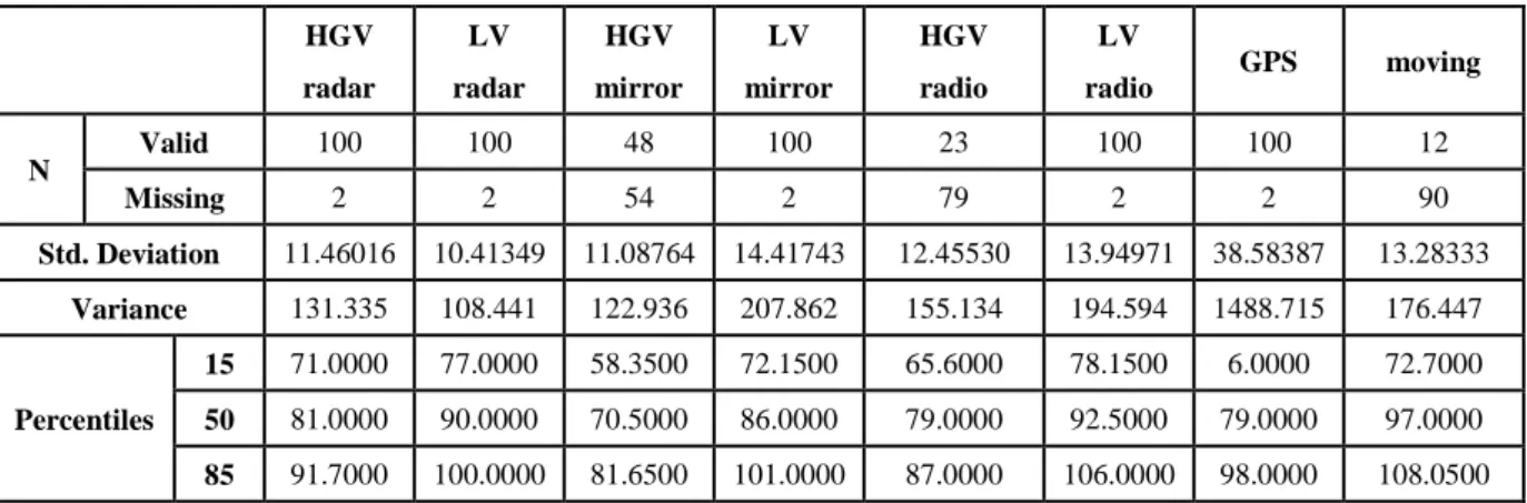
Table 3-2 Descriptive analysis

HGV radar LV radar HGV mirror LV mirror HGV radio LV radio GPS moving N Valid 100 100 48 100 23 100 100 12 Missing 2 2 54 2 79 2 2 90 Std. Deviation 11.46016 10.41349 11.08764 14.41743 12.45530 13.94971 38.58387 13.28333 Variance 131.335 108.441 122.936 207.862 155.134 194.594 1488.715 176.447 Percentiles 15 71.0000 77.0000 58.3500 72.1500 65.6000 78.1500 6.0000 72.7000 50 81.0000 90.0000 70.5000 86.0000 79.0000 92.5000 79.0000 97.0000 85 91.7000 100.0000 81.6500 101.0000 87.0000 106.0000 98.0000 108.0500

HGV= Heavy Goods Vehicle, LV= Light Vehicle

As the table shown above, the attributes of the results of each categories could be achieved from the descriptive analyse, including standard deviation, mean, median, mode, variance and percentiles (15%, 50% and 85%).

3.3 Comparison

3.3.1 The distribution of speeds and normal distribution

To compare the distribution of speeds and normal distribution, there are two ways for analysing, such as the histogram and Chi-square test.

The histogram which is sketched out by SPSS can generally illustrate the distribution. The vertical axis is the frequency of each group of speeds; and the horizontal axis represents the speeds of the vehicles in each category. The graphs (Figure 3-1 ~ 3-8) which are shown below are in five groups (Radar, Mirror, Radio，GPS and Moving vehicle), whilst each one is comprised of heavy vehicle and light vehicle (excluding GPS and Moving vehicle). The normal distribution curve of each measurement was also included so that the comparison could be achieved legibly.

110.00 100.00 90.00 80.00 70.00 60.00 50.00 40.00 HG Vra d a r 20 15 10 5 0 F re que nc y Me a n = 81.09 S td. De v. = 11.46016 N = 100 HG Vra d a r 120.00 110.00 100.00 90.00 80.00 70.00 60.00 LVra d a r 25 20 15 10 5 0 F re que nc y Me a n = 88.94 S td. De v. = 10.41349 N = 100 LVra d a r

Heavy vehicle Light vehicle

Figure 3-1 and 3-2 Radar

100.00 90.00 80.00 70.00 60.00 50.00 HG Vm irro r 10 8 6 4 2 0 F re que nc y Me a n = 70.8542 S td. De v. = 11.08764 N = 48 His to g ra m 130.00 120.00 110.00 100.00 90.00 80.00 70.00 60.00 LVm irro r 20 15 10 5 0 F re que nc y Me a n = 87.58 S td. De v. = 14.41743 N = 100 His to g ra m

Heavy vehicle Light vehicle

Figure 3-3 and 3-4 Mirror

120.00 110.00 100.00 90.00 80.00 70.00 60.00 50.00 H G Vra d io 8 6 4 2 0 F re que nc y Me a n = 78.0435 S td. De v. = 12.4553 N = 23 His to g ra m 130.00 120.00 110.00 100.00 90.00 80.00 70.00 60.00 LVra d io 20 15 10 5 0 F re que nc y Me a n = 92.54 S td. De v. = 13.94971 N = 100 His to g ra m

Heavy vehicle Light vehicle

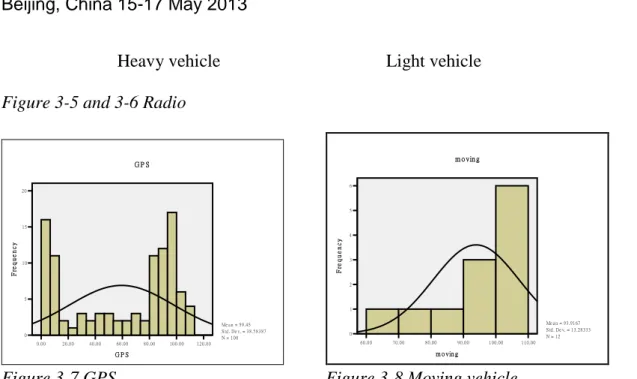
Figure 3-5 and 3-6 Radio

120.00 100.00 80.00 60.00 40.00 20.00 0.00 G P S 20 15 10 5 0 F re que nc y Me a n = 59.45 S td. De v. = 38.58387 N = 100 G P S 110.00 100.00 90.00 80.00 70.00 60.00 m o vin g 6 5 4 3 2 1 0 F re que nc y Me a n = 93.9167 S td. De v. = 13.28333 N = 12 m o vin g

Figure 3-7 GPS Figure 3-8 Moving vehicle

As the figures shown above, because the obvious differences between the normal distribution curve and histogram of GPS (Figure 3-7) and Moving vehicle (Figure 3-8), the two sets of data could be concluded that the normal distribution has not been accommodated.

However, the accurate results of the rest of figures are difficult to be obtained only from the illustrations due to the different visibility of various observers. Alternatively, the chi-square goodness-of-fit test has been introduced for testing the normalcy of the speed data according to statistic theory (McShane, Prassas and Roess 1998:166). Thereby, the chi-square test was mainly concerned with through out the analysis so that the probability of mistakes could be reduced, and the results should more stringent.

The main equation used in the chi-squared test explained by McShane et al. (1998:166) “ 2 2 ( i i) N i n e X e − =

∑

Where: ei = theoretical frequency of observations in a particular speed group, assuming a normal distribution.

ni = observed frequency of observations in a particular speed group, from field data N = number of speed groups used”

The results of chi-squared are presented following.

Table 3-3 chi-square goodness-of-fit test

chi-square value Prob. reject accept

Radar Heavy vehicle 18.3868 ＜0.5% √

Mirror Heavy vehicle 2.15246 54.63% √

Light vehicle 9.4341 23% √

Radio Heavy vehicle 2.1658 15.8% √

Light vehicle 8.6998 28% √

To estimate the distribution of each measurement is consistent with the normal distribution, the probability of X2 should be less or equal to 5% (McShane, Prassas and Roess 1998:166). As illustrated in table 3-3, compared with the probability of each category, only the heavy vehicle speed group of radar measurement is less than 0.5%; in the other words, the normal distributions can not be satisfied with that of the rest of categories.

3.3.2 The results and the automatic traffic counter

The speeds observed by automatic traffic counter are classified into Class 1, 2, 3 and 4. Class 1 represents heavy vehicle, and the rest of them mean light vehicle; therefore the data processing was also consistent with the previous two types (heavy and light). According to the sample size determined in section3.2.1, the 100 data have been selected from the two groups both lane1 and 2. After data processing, the results could be achieved, and the table below includes not only the important attributes of ATC, but also that of the previous measurements.

Table 3-4 attributes of all measurements

TMS (km/hr) SMS (km/hr) Percentile speed Std. Deviation 15% 85% ATC HV 77 76 67 88 9.7699 ATC LV 71 71 63 79 7.7974 Radar HV 81 79 71 91.7 11.4602 Radar LV 89 88 77 100 10.4135 Mirror HV 71 69 58.35 81.65 11.0876 Mirror LV 85 88 72.15 101 14.4174 Radio HV 78 76 65.6 87 12.4553 Radio LV 93 91 78.15 106 13.9497 GPS 59 17 6 98 38.5839 Moving vehicle 94 92 72.7 108.05 13.2833

HGV= Heavy Vehicle, LV= Light Vehicle

Moreover, the histograms (including normal distribution curves) of both types of vehicles also could be obtained by SPSS.

120.00 100.00 80.00 60.00 40.00 H V 14 12 10 8 6 4 2 0 F re que nc y Me a n = 77.14 S td. De v. = 9.76183 N = 100 HV 90.00 80.00 70.00 60.00 50.00 LV 20 15 10 5 0 F re que nc y Me a n = 71.38 S td. De v. = 7.7886 N = 100 LV

Heavy vehicle Light vehicle

Figure 3-9 and 3-10 ATC

4 DISCUSSION ON RESULTS

4.1 Results from the speed data

The results of time mean speed and space mean speed for all the five measurements have been shown in table 3-1. The same results have been achieved from radar, radio and mirror measurements that both time mean speed and space mean speed of light vehicle groups are higher than that of heavy vehicles. As standards for estimating the lowest and highest speed limitation, the 15% and 85% percentile speeds (see table 3-3) calculated from both two groups, the same conclusion could be made as well. However, the four results obtained from GPS observer are all the lowest compared with the other four measurements; importantly, the values are unreasonably lower than the others. According to the tabulated data in the appendix1.4, more than 20% of speed data collected from GPS measurement is below 10km/h, it should be the main reason for this problem.

In the table 3-3, the standard deviation of each measurement also has been included. Except for the GPS method, the other four values range from 10 to 15. The value of GPS is approximate three times than the others. That could be translated that the speed data of GPS is much more dispersed from the mean. Similarly as the reason stated in the time mean speed and space mean speed analysis, the speed data which is less than 10km/hr should be the critical factor caused the unexpected high.

In the comparison between distribution of each measurement and normal distribution, although based on the illustration comparing and chi-square goodness-of-fit test, only the curve of heavy vehicle of radar measurement is approximately consistent with normal distribution curve, the figure 3.7(GPS) still has illustrated the unanticipated result from GPS speed data.

4.2 Methods

Although the results could be calculated from the data observed by the five various measurements, the differences and accuracy of them still exist due to their operations, the physical environment, external factors and so on.

The radar gun is the one of the most convenient and fastest ways to collect the spot speeds of the vehicles on the road. The speeds could be displayed while facing the vehicle immediately. Whereas, the accuracy has been discussed (McShane, Prassas and Roess 1998:158) that as the time the observers have been known by drivers, it could be influenced. And the operation process could be also the factor leads to the unexpected errors, such as the location of the observation, the directions opposite to the coming vehicles.

During the Mirror and the Radio methods, the errors could be generated from the determination of the stop/end line, the communication between the operators, and the delays in the readings. However, the mirror measurement adopts the reflection theory in optics to improve the visibility of the stop and finish reference; consequently, this error could be avoided by the mirror measurement. Compared with the radar gun method, the selection of the vehicles could have high continuity because of the less delay occurred during the readings.

Since the precise coordinate and accurate time could be easily obtained by GPS simultaneously, the GPS should be the most accurate measurement among them. But the distribution and the processed speed data have illustrated that there are some unanticipated speeds have been collected, and they have resulted in the large difference between the distribution of GPS speed data and normal distribution curve. According to the data shown in appendix 1.4 (GPS), the speeds less than 10km/hr could be detected wrongly due to the external environment factors. Compared with observing speeds manually, the problem could not be easily solved during the readings, and the unexpected could be treated as outliers sometimes so that they would not affect the accuracy of the distribution.

The moving vehicle measurement was carried out with the GPS observer together in the field work. One of the disadvantages has been stated (Guest, Matthews and Slinn 2005:24) that the chances for overtaking could not be achieved during the high occupancy of roads. During the observation, the traffic was in good condition; hence, the moving vehicle method was practical.

4.3 Automatic traffic counter (ATC)

Based on the table 3-4, the standard deviations of both two types of ATC are lower than that of other measurements; it could be translated that the central tendency will be better in distributions of the ATC compared with the other measurements. The result could be also achieved from the figure 3-9 and 3-10. And in terms of the two illustrations, the conclusion could be also made that the distributions of the ATC are more consistent with the normal distribution. Therefore, the description of the ATC should be more precisely than that of the five methods.

5 CONCLUSION

In this report, the aims are focused on exploring the characteristics of each measurement adopted in the field work and the analysis of the observed speed data. The results of the comparison among the five methods indicate that the radar and GPS are more convenient to measure the speed; however, compared with the radio and mirror measurements, the external environmental factors could be hard to be avoided so that the unexpected speeds exist in the data processing. Moreover, the attributes and distributions of each measurement have been achieved applying statistics cooperated with relevant software. Comparing the histogram of ATC and goodness-of-fit test results with that of the methods carried out in the field work, it could be concluded that the speed data of ATC are more representative of the traffic condition due to the better normalcy. According to the discussion in the fourth section, the unexpected speeds were observed because of manual or mechanical problems, therefore the operations could be strictly in accord with the requirements of each measurement; during the data processing, the statistics should be applied properly, especially the determination of sample size should be taken more consideration, and the coefficients should be selected in terms of different requirements of the analysis.

REFERENCES

Guest, P., P. Matthews and M. Slinn (2005) Traffic Engineering Design: Principles and Practice (2nd Edition). Oxford: Elsevier Ltd.

McShane, W. R., E. S. Prassas and R. P. Roess (1998) Traffic Engineering (2nd Edition). New Jersey: Prentice-Hall, Inc.