Journal of Neuroscience Methods 347 (2021) 108951
Available online 2 October 2020
0165-0270/© 2020 The Authors. Published by Elsevier B.V. This is an open access article under the CC BY license (http://creativecommons.org/licenses/by/4.0/).
Invited review
The sensitivity of diffusion MRI to microstructural properties and
experimental factors
Maryam Afzali
a,*
, Tomasz Pieciak
b,c, Sharlene Newman
d,e, Eleftherios Garyfallidis
e,f,
Evren ¨Ozarslan
g,h, Hu Cheng
d,e, Derek K Jones
aaCardiff University Brain Research Imaging Centre (CUBRIC), School of Psychology, Cardiff University, Cardiff, United Kingdom bAGH University of Science and Technology, Krak´ow, Poland
cLPI, ETSI Telecomunicaci´on, Universidad de Valladolid, Valladolid, Spain
dDepartment of Psychological and Brain Sciences, Indiana University, Bloomington, IN 47405, USA eProgram of Neuroscience, Indiana University, Bloomington, IN 47405, USA
fDepartment of Intelligent Systems Engineering, Indiana University, Bloomington, IN 47408, USA gDepartment of Biomedical Engineering, Link¨oping University, Link¨oping, Sweden
hCenter for Medical Image Science and Visualization, Link¨oping University, Link¨oping, Sweden
A R T I C L E I N F O Keywords: Diffusion MRI Signal representation Biophysical model Microstructure Experimental factors Anisotropy A B S T R A C T
Diffusion MRI is a non-invasive technique to study brain microstructure. Differences in the microstructural properties of tissue, including size and anisotropy, can be represented in the signal if the appropriate method of acquisition is used. However, to depict the underlying properties, special care must be taken when designing the acquisition protocol as any changes in the procedure might impact on quantitative measurements. This work reviews state-of-the-art methods for studying brain microstructure using diffusion MRI and their sensitivity to microstructural differences and various experimental factors. Microstructural properties of the tissue at a micrometer scale can be linked to the diffusion signal at a millimeter-scale using modeling. In this paper, we first give an introduction to diffusion MRI and different encoding schemes. Then, signal representation-based methods and multi-compartment models are explained briefly. The sensitivity of the diffusion MRI signal to the microstructural components and the effects of curvedness of axonal trajectories on the diffusion signal are reviewed. Factors that impact on the quality (accuracy and precision) of derived metrics are then reviewed, including the impact of random noise, and variations in the acquisition parameters (i.e., number of sampled signals, b-value and number of acquisition shells). Finally, yet importantly, typical approaches to deal with experimental factors are depicted, including unbiased measures and harmonization. We conclude the review with some future directions and recommendations on this topic.
1. Introduction
The classical way of studying microstructural information of tissue is histology. This method has some limitations; it needs a biopsy, tissue preparation, the samples are small, and longitudinal measurements of the same sample are not easy (Gurcan et al., 2009). Diffusion MRI, on the other hand, can provide information about tissue microstructure non-invasively (Le Bihan et al., 1988). The advantages of the technique compared to histology are that it does not need a biopsy or tissue preparation, is a non-invasive technique, and is easy to run repeated measurements (Basser et al., 1994b; Le Bihan, 2003; Jones, 2010). The
imaging field-of-view can be large enough to cover the whole organ instead of imaging only a small sample of the tissue. The data acquisition is faster than analysis of histology sections (Alexander et al., 2019).
Histological studies have provided a lot of knowledge about brain microstructure and connectivity (Braak and Braak, 1995). The very first works in this area began with post-mortem tissue (Schulz et al., 1980). The non-invasive nature of diffusion MRI makes it feasible to study brain microstructure in healthy volunteers as well as patients (van Gelderen et al., 1994; Fazekas et al., 1987; Shenton et al., 1992). The acquisition of data on a population is possible and therefore group analysis studies are feasible (Afzali et al., 2011). It is also possible to make repeated
* Corresponding author.
E-mail addresses: AfzaliDeliganiM@cardiff.ac.uk (M. Afzali), tpieciak@gmail.com (T. Pieciak), sdnewman@indiana.edu (S. Newman), elef@indiana.edu (E. Garyfallidis), evren.ozarslan@liu.se (E. ¨Ozarslan), hucheng@indiana.edu (H. Cheng), JonesD27@cardiff.ac.uk (D.K. Jones).
Contents lists available at ScienceDirect
Journal of Neuroscience Methods
journal homepage: www.elsevier.com/locate/jneumeth
https://doi.org/10.1016/j.jneumeth.2020.108951
measurements in the study of brain development or ex-vivo studies (Roebroeck et al., 2019) and in pathological disorders, preventing the risk and side-effects of the biopsy (Kreth et al., 2001). The study of the whole organ is possible preventing the false-negative effect due to sampling the wrong part of the tissue.
The level of anatomical detail in histology studies is much higher than in microstructure imaging techniques. The submicron resolution in histology/electron microscopy provides insight into the cellular struc-ture of the tissue while the millimeter resolution of diffusion MRI pro-vides statistical descriptions of the tissue. In some cancer studies, information at the cellular level is useful while in some other biomedical applications, being able to detect statistical changes in the tissue is useful (Mouras et al., 2010). For example, the size distribution of axons in white matter determines the conduction velocity (Drakesmith et al., 2019). Different shapes and configurations of the cells can indicate the type of tumor (Kauppinen, 2002).
Diffusion MRI provides a tool to study brain tissue based on the Brownian motion of water molecules (Tanner, 1979; Le Bihan et al., 1988) and it is therefore sensitive to differences in the microstructure of the tissue (Callaghan et al., 1988; Basser et al., 1994b; Jones, 2010). In this technique, the images are acquired with different number of di-rections, b-values, b-tensor encoding schemes (Callaghan et al., 1988; Basser et al., 1994b; Jones, 2010; Westin et al., 2016). Then a model is fitted to the signal and a set of parameters can be obtained for each voxel in the image—either for signal representations (e.g. DT-MRI) (Basser et al., 1994b) or modelling (Stanisz et al., 1997). These parameters are related to the microstructural properties of the tissue. Diffusion MRI sensitizes the signal to the random motion of the water molecules in a diffusion time from millisecond up to one second. At room or body temperature, the mean displacement due to motion over this time-scale is at the scale of the micrometer, which is the cellular scale. Therefore the cellular structure of the tissue directly affects the motion of the water molecules, so diffusion MRI is a useful tool to study the tissue microstructure.
Diffusion MRI has found a lot of applications in biomedical imaging in recent years. This work reviews the sensitivity of the diffusion signal to the microstructure of the underlying tissue and the experimental factors. Therefore, we focus on signal representation techniques as well as biophysical modeling (Novikov et al., 2019). In this review, we will explain how the signal is sensitive to the underlying microstructure and how it can be misinterpreted in the presence of noise and various experimental factors. In Section 2 we explain brain microstructure briefly. In Section 3 we provide some background information about the diffusion MRI signal and different encoding schemes. In Section 4 we focus on diffusion signal representation-based methods and then in Section 5 we introduce multi-compartment models, the sensitivity of the signal to the axon diameter, size distribution, and curvedness of neural trajectories. Furthermore, we present the limitations of multi-compartment models and present the inherent effects of model fitting procedures. Next, in Section 6, we explain the effect of noise and present typical experimental factors that might affect diffusion MRI studies. Finally, in the last section, we conclude the review and give some hints and tips for future directions.
2. Brain microstructure
The brain contains neurons and glial cells and has three main parts; white matter (WM), gray matter (GM), and cerebrospinal fluid (CSF). The gray matter includes cell bodies and dendrites. White matter is mainly composed of densely packed axons that emerge from the soma in the GM. Glial cells are also present in the WM (Buzs´aki et al., 2013). The diameter of dendrites is around 0.2–3 μm. The structure of the dendritic
branches depends on the type of neuron (Fiala et al., 2007). A few dendrites (less than five) emerge directly from the soma. In the cerebral cortex the branches of the dendritic tree are isotropically distributed while in other regions such as the hippocampus, they are anisotropic
(Zaqout and Kaindl, 2016). The length of axons in the human brain changes from a few millimeters in intra-cortical connections to around 1 meter in the corticospinal pathway (Schüz and Braitenberg, 2002). In the WM the axon diameter ranges from 0.1 to 10 μm (Aboitiz et al.,
1992; LaMantia and Rakic, 1990; Ong et al., 2008; Waxman and Ben-nett, 1972; Drakesmith et al., 2019). The axon diameter distribution (ADD) is different in different species (Innocenti et al., 2014, 2016; Caminiti et al., 2009). When modeling axon diameters, a gamma dis-tribution is normally assumed for this disdis-tribution (Sepehrband et al., 2016a; Assaf et al., 2008) though alternative distributions have been considered based on optimal information flow subject to relevant con-straints (Pajevic and Basser, 2013). The mean of the ADD containing the myelinated axons is around 0.5–0.8 μm. Most of the diffusion-based
ADD measurements, to date, have been made in the mid-sagittal corpus callosum (CC). The reason is that the fibers in the callosum are most co-aligned and this makes the orientation known and reduces the complexity of the modeling. The mid-body has a larger mean ADD than the genu, the smallest ADD in CC is observed in splenium (Aboitiz et al., 1992; LaMantia and Rakic, 1990; Caminiti et al., 2009; Riise and Pak-kenberg, 2011). In mammals, the brain connection through the mid-body has larger axons (Caminiti et al., 2009).
The myelin contains 80% lipids and 20% proteins with 10 nm thickness wrapping the axons. The myelin divides into segments, the spaces between the segments are the nodes of Ranvier. The length of segments is around 0.2–2 mm (Rushton, 1951) while the length of nodes is 1–2 μm (Salzer, 1997). The myelin increases the conduction velocity
(Waxman and Bennett, 1972; Rushton, 1951). The inner diameter of the myelinated axon to the outer diameter of the myelinated axon is called g-ratio and in normal CNS it is around 0.7 (Smith and Koles, 1970). In the CC most of the axons are myelinated. In the genu, the amount of unmyelinated axons is around 16–20% (Aboitiz et al., 1992; LaMantia and Rakic, 1990). The central nervous system contains glial cells. In human adult, the glial cells fall into three categories: 76.6 % oligoden-drocytes, 17.3% astrocytes, and 6.5% microglia in number (Pelvig et al., 2008; Salvesen et al., 2017). Oligodendrocytes create the myelin sheaths around axons (Baumann and Pham-Dinh, 2001). Astrocytes have somas with a diameter around 10 μm which generates a star-shaped structure.
They are responsible for tissue repair and balancing the amount of extracellular ions (Ding et al., 2016). Microglia provide the first reaction after an injury (see Gehrmann et al., 1995) and their soma is approxi-mately 10 μm in diameter.
In the white matter, there are intra-axonal and extra-cellular spaces. The intra-axonal space is the space-separated by the membrane of axons. In axons, filaments preserve the shape and organization of axons and provide support for the intra-axonal transportation system. Microtu-bules are part of the cytoskeleton and they aid in transportation. The diameter of the microtubules is around 25 nm. The density of microtu-bules is related to the axon diameter (Fadi´c et al., 1985).
In addition to intra-axonal space, there is also extra-cellular space that surrounds cells, axons, and dendrites. The amount of extracellular volume fraction in the non-human brain is reported as 15–35% using invasive microscopy (Sykov´a and Nicholson, 2008). But the shrinkage effect of this microscopy has been reported as 1–65% (Aboitiz et al., 1992; LaMantia and Rakic, 1990; Riise and Pakkenberg, 2011; Houzel et al., 1994).
The images acquired using diffusion MRI are at the scale of mm while the features that we are interested in such as anisotropy, cell size, and axon diameter are at the scale of the micrometer. Each voxel may contain hundreds of thousands of axons that may bend, fan, or cross which makes the modeling of the geometry of the axons complicated.
3. Different acquisition schemes
Time-varying magnetic field gradients are incorporated into MR pulse sequences for encoding diffusion. The most commonly used scheme was introduced by Stejskal and Tanner (1965), which employs a
pair of pulsed magnetic field gradients around the 180∘ radiofrequency
pulse in a spin-echo measurement as illustrated in Fig. 1a. We adopt the nomenclature in Shemesh et al. (2016) and refer to such a Pulsed Gradient Spin Echo (PGSE) sequence by single diffusion encoding (SDE). It should be noted, however, that the method can be incorporated into sequences other than spin-echo based ones. Since its introduction (Stejskal and Tanner, 1965), there have been different works aimed at maximizing the information that can be obtained from a dMRI experi-ment by exploring different acquisition protocols (Jones, 2004; Alex-ander, 2008; Alexander et al., 2019).
In SDE, the MR signal is sensitized to diffusion using a pair of gradient pulses that encode the position of the spins along the axis defined by the diffusion gradients. In this sequence, the magnetic field gradient is applied in the direction g where the pulse duration is δ and the time between the leading edges of the two pulses is Δ which de-termines the diffusion time (see Fig. 1a). The diffusion of water mole-cules between and during the pulses attenuates the signal. This attenuation increases when the molecules have a larger displacement between the two pulses.
For free diffusion, the diffusion coefficient can be estimated directly from the signal attenuation based on δ, Δ, and gradient strength. In
restricted diffusion, however, the displacement is limited and the signal attenuation is smaller than that for free diffusion. The signal attenuation in a restricted medium depends on the size and shape of the pore as well as the parameters of the sequence such as δ, Δ, and G (gradient strength). By varying the experimental parameters one attempts to obtain the geometric features of the pore (Assaf et al., 2000; Stanisz et al., 1997; Åslund et al., 2009). These parameters are typically collapsed into the so-called the b-value. The b-value determines the diffusion weighting of a sequence and for SDE is given by b = γ2δ2G2(Δ − δ/3) (Stejskal and Tanner, 1965), where γ is the gyromagnetic ratio. The ramp time of the pulse is neglected here. For free diffusion, the b-value is sufficient to determine the signal attenuation, which is not sensitive to changes in the timing parameters of the signal as long as they generate the same
b-value. For free diffusion, the signal exhibits a monoexponential decay
according to
S(b) = S(0)exp( − bD), (1)
where D is the (scalar) diffusion coefficient. In the presence of restricted diffusion, the signal attenuation depends on the timing parameters of the sequence even though they might provide the same b-value.
Some other types of SDE can provide some practical benefits. For
Fig. 1. Diffusion acqusition schemes: (a) pulsed gradient spin-echo (PGSE), double diffusion encoding sequence (DDE) and oscillating diffusion encoding (ODE). For more details about diffusion MRI sequences see Table 1 and Section 3.
example, using asymmetric gradients or twice-refocused spin-echo se-quences can reduce the effect of eddy currents (Reese et al., 2003; Fin-sterbusch, 2009a). Using pulsed-gradient stimulated-echo sequences (PGStE) (Callaghan, 1991) provides longer diffusion times compared to the pulsed gradient spin-echo (PGSE) sequence at the cost of half the signal-to-noise ratio (SNR). In PGSE, the minimum echo time (TE), and therefore minimum T2-signal loss, is dictated by the diffusion time and
the duration of the gradients. PGSE contains a 90◦ and a 180◦
radio-frequency pulse while PGStE has three 90◦pulses to excite, store
and recall the magnetization (Tanner, 1970; Merboldt et al., 1985). In PGStE, only T1 relaxation occurs between the second and the third 90◦
pulses, which is typically slower than the T2 relaxation that attenuates
the PGSE signal. Therefore, PGStE can provide a larger signal amplitude at a longer diffusion time. The limitation of PGStE is that half of the SNR is lost in the storage and recall process (Callaghan, 1991; Schick, 1998). Therefore, PGStE is preferred over PGSE when long diffusion times are desired (Ozarslan et al., 2012¨ ) and for tissue in which the T2 is relatively
short (e.g., muscle). Another type of SDE employs gradient pulses of different durations, providing sensitivity to the pore shape (Laun et al., 2011).
In addition to the size and shape of the cells, other properties such as exchange, intra-voxel incoherent motion (IVIM), and fiber density are among the quantities and phenomena that influence the signal. Each voxel may contain several compartments, including cell bodies, intra- axonal and extra-cellular spaces, and glial cells. Using multi-shell ac-quisitions, one may be able to extract the anisotropy and density of different compartments (Kaden et al., 2007; Jespersen et al., 2007). The size of the compartments can be estimated by changing the diffusion time in SDE acquisitions (Callaghan, 1993; Packer and Rees, 1972). Compared to full restriction, if there is an exchange between compart-ments, the signal attenuation increases with increasing diffusion time. In practice, an increase in the restriction size has a similar effect as ex-change and therefore it is not easy to disentangle them from each other using SDE (Nilsson et al., 2010). For low b-values, the SDE signal con-tains the effect of perfusion (IVIM) (Le Bihan et al., 1988).
Another useful sequence is Double Diffusion Encoding (DDE) which contains two pairs of pulsed-field gradients that are separated from each other with a mixing time τ (see Fig. 1b) (Cory et al., 1990; Callaghan, 2011). An alternative realization to this sequence involves overlapping the two pulses in the middle to realize short τ values when narrow pulses
are not feasible (Ozarslan and Basser, 2008¨ ). It has been shown that
DDE, as well as other multiple encoding schemes (Ozarslan and Basser, ¨ 2007; Finsterbusch, 2009b; Avram et al., 2013) such as Triple Diffusion Encoding (TDE) (Topgaard, 2017; Ramanna et al., 2020), provide in-formation that is not accessible with single diffusion encoding (Mitra, 1995; Cheng and Cory, 1999; ¨Ozarslan and Basser, 2007). This approach has been utilized by several groups for extracting microstructural in-formation (Ozarslan et al., 2009b; Jespersen et al., 2013; Benjamini ¨ et al., 2014; Ianus¸ et al., 2016; Yang et al., 2018; Coelho et al., 2019). Varying the relative gradient directions of the two SDE blocks, one is
able to estimate microscopic diffusion anisotropy (Cheng and Cory, 1999; ¨Ozarslan, 2009; Finsterbusch, 2011; Jespersen et al., 2013; She-mesh, ¨Ozarslan et al., 2010a) whereas varying the gradients’ strengths while keeping them orthogonal to each other reveals compartmental kurtosis (Paulsen et al., 2015). In order to estimate exchange, e.g. through the membrane between extra-cellular and intra-cellular spaces, parallel gradients with variable mixing time can be used (Furo and Dvinskikh, 2002; Åslund et al., 2009; Lasiˇc et al., 2011; Sønderby et al., 2012; Nilsson et al., 2013; Ning et al., 2018). In this experiment, the first pair of pulsed-field gradients differentially attenuates the signals in the two compartments, assuming that their diffusivities are different and this gradually returns to equilibrium. To measure exchange, the mixing time is increased gradually and the second block of gradients is used to monitor this equilibrium. Another application of DDE is the estimation of compartment size using parallel and antiparallel gradients with a short mixing time (Koch and Finsterbusch, 2008; Finsterbusch, 2011).
Oscillating diffusion encoding (ODE) can be achieved by changing the single pulsed gradient on either side of the 180◦RF pulse to a series
of pulsed gradients having the oscillating form (see Fig. 1c) (Callaghan and Stepiˇsnik, 1995). Estimation of the diffusivity in small compart-ments needs short diffusion times using SDE, this limits the b-value that can be achieved and therefore decreases the sensitivity to microscopic features. By repeating multiple pulses in ODE, one can maintain a high
b-value at short diffusion times. This improves the sensitivity to diffusion
coefficients in small pores and therefore the feasibility of estimating small pore sizes (Gore et al., 2010; Xu et al., 2014). The ODE is useful for the estimation of axon diameters in the presence of orientation disper-sion because it provides a low signal from free diffudisper-sion along the cyl-inder axis and retains sensitivity to the size (Drobnjak et al., 2016; Nilsson et al., 2017).
Although SDE, DDE, and ODE are the most common gradient waveforms there is no reason to limit the shape of the gradient to a rectangular/trapezoidal waveform. Having free gradient waveforms may be more useful than the trapezoidal ones (Drobnjak and Alexander, 2011; Drobnjak et al., 2010). One example is double oscillating diffusion encoding (DODE), which can enhance the estimation of size and shape (Ianus¸ et al., 2017; Ianus¸ et al., 2018). Another category is multiple diffusion encoding to disentangle microscopic anisotropy from isotropic diffusion, which is not feasible using SDE alone (Mitra, 1995). A framework called q-space trajectory imaging (QTI) was recently intro-duced by Westin et al. (2016) to probe tissue using different gradient waveforms. The traditional, pulsed field gradient sequences attempt to probe a point in q-space but in q-space trajectory encoding, time-varying gradients are used to probe a trajectory in q-space. By employing a diffusion tensor distribution model (Jian et al., 2007), the QTI frame-work provides some microstructural information that is not available in traditional pulsed gradient encoding proposed by Stejskal and Tanner. In multi-dimensional diffusion MRI, the b-matrix is defined as an axisymmetric second order tensor (Topgaard, 2017)
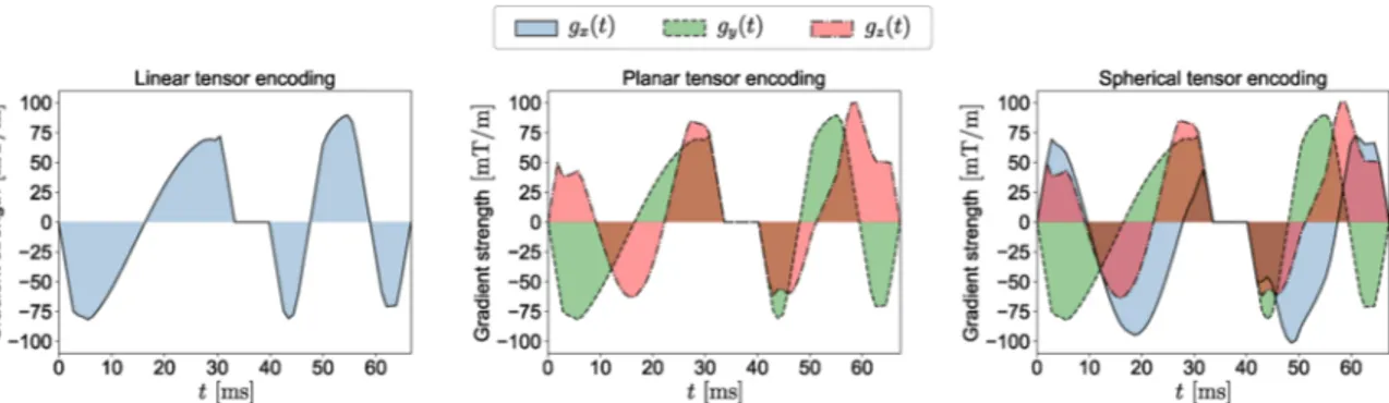
Fig. 2. The free gradient waveforms g(t) =[gx(t), gy(t), gz(t) ]T
of the linear, planar, and spherical tensor encoding. For more details about the gradient waveforms see Section 3.
B = b(1 − bΔ )
I3 /
3 + bbΔggT, (2)
where I3 is the identity matrix, g is the diffusion gradient direction and
the b-value, b, is defined as the trace of the b-matrix. The eigenvalues of the b-matrix are b∣∣, b(1)⊥ and b(2)⊥ where b⊥(1)=b(2)⊥ =b⊥ and b∣∣ is the
largest. bΔ is defined as bΔ =(b∣∣ − b⊥)/(b∣∣ +2b⊥). In this framework,
SDE and ODE are just special realizations of linear tensor encoding (LTE;
Fig. 2) where the b-tensor has only one non-zero eigenvalue as all gra-dients are in the same orientations. DDE is a special case of planar tensor encoding (PTE; Fig. 2) as all gradients line on a plane and the b-tensor has two non-zero eigenvalues. In spherical tensor encoding (STE; Fig. 2) the gradients may point in all directions giving rise to a rank-3 b-matrix. Changing bΔ, we can generate different types of b-tensor encoding. For
LTE, PTE, and STE, bΔ =1, − 1/2, and 0 respectively (see Topgaard,
2017).
In Table 1 we summarize diffusion encoding schemes aforemen-tioned in this section and provide the information they reveal.
4. Signal representations
Most diffusion MRI based analysis of microstructure falls into two categories: a model of the signal to compute quantitative physical properties of the diffusion and representations of the tissue to acquire tissue-specific metrics. Techniques based on the representation of the signal focus on delineating the diffusion signal attenuation without explicitly considering the underlying tissues that create this attenuation (Basser et al., 1994b; Descoteaux et al., 2011; Jensen et al., 2005; Merlet and Deriche, 2013; ¨Ozarslan et al., 2013; Tournier et al., 2011; Ning et al., 2015b; Fick et al., 2016). The most widely used, DT-MRI, employs
a tensor to characterize the Gaussian distribution of displacements and MRI signal decay (Basser et al., 1994b,a). DT-MRI (Basser et al., 1994b) has been widely used to determine anisotropy in the tissue in vivo. The microstructure of the tissue can be used to determine the effect of aging (Abe et al., 2002), mild traumatic brain injury (Shenton et al., 2012), or some diseases of the central nervous system such as schizophrenia and Alzheimer’s disease (Kubicki et al., 2007; Alexander et al., 2019) or even in the preoperative evaluation of tumor grade (Inoue et al., 2005). DT-MRI can provide noninvasive markers of tissue state (Pierpaoli and Basser, 1996) and also can map anatomical connections between different regions of the brain (Mori et al., 1999; Conturo et al., 1999; Basser et al., 2000).
DT-MRI is obtained when the Maclaurin series representation of the natural logarithm of the MR signal is terminated after the first term. Such an expansion is sometimes referred to as the cumulant expansion as the coefficients of different terms correspond to the cumulants of the net displacement distribution (Liu et al., 2004). While the first term, hence the diffusion tensor, is related to the covariance (Basser, 2002), the next term in the series contains the kurtosis of this distribution. Diffusion Kurtosis Imaging (DKI) is obtained when the kurtosis term in addition to the covariance term is preserved in the expansion (Jensen et al., 2005). Doing so extends the validity of the representation towards larger
b-values. More importantly, a measure of Generalized Kurtosis is
pro-vided, which is a 3-dimensional equivalent of the 1-dimensional kurtosis measure used in the DKI literature. However, complex white matter structures such as fiber crossing, bending and branching can obscure the true kurtosis measurements. There are some researches that extend DKI in microstructural environments with orientation heterogeneity (Ankele, 2019; Huynh et al., 2019b; Ankele and Schultz, 2015) and show
Table 1
Summary of diffusion encoding schemes and information they reveal. Each gradient waveform can be incorporated into spin echo or stimulated echo sequences where the latter is preferred for long diffusion times particularly for species in which T2 is relatively short (e.g., muscle) (Callaghan, 1991).
Encoding Sequence Applications Advantages Disadvantages Reference
Single SDE Measuring free and restricted diffusion Easy to implement Non-optimized in measuring some microstructural features of the tissue
(Stejskal and Tanner, 1965; Huynh
et al., 2020; Kaden et al., 2016a)
Ensemble average propagator (K¨arger and Heink, 1983)
Diffraction-like features (Callaghan et al., 1991)
Modeling anisotropic diffusion, Diffusion tensor
imaging (Basser et al., 1994b)
Fiber-tract mapping (Mori et al., 1999)
Mapping Connectomes (Sotiropoulos and Zalesky, 2019)
Neurosurgery, Neuro-oncology (Panesar et al., 2019; Potgieser et al.,
2014)
ODE Diffusivity in small compartments, axon diameter (Callaghan and Stepiˇsnik, 1995)
Double DDE Microscopic diffusion anisotropy (Cory et al., 1990; Cheng and Cory,
1999)
Compartment size and disambiguation of free and
restricted diffusion Sensitive to microscopic anisotropy Long acquisition time and long TE compared to SDE
(Mitra, 1995)
Exchange between different compartments (Callaghan et al., 2003)
Compartmental kurtosis (Paulsen et al., 2015)
DODE Enhances the estimation of size and shape (Ianus¸ et al., 2017)
Multiple MDE Isotropic (spherical tensor) encoding for direct
measurement of the trace of the diffusion tensor Sensitive to microscopic anisotropy Long acquisition time (Mori and van Zijl, 1995)
Same as DDE with potential advantages (Ozarslan and Basser, 2007; ¨
Finsterbusch, 2009b; Topgaard, 2017)
Free
waveform QTI Microscopic and macroscopic diffusion anisotropy, size variance, orientational coherence Short echo time compared to DDE and MDE Complicated gradient waveforms, long TE compared to SDE, diffusion time is ill-defined in time domain, needs spectrally matched waveforms for comparison (Lundell et al., 2019) (Westin et al., 2016)
Acronyms: SDE – single diffusion encoding, ODE – oscillating diffusion encoding, DDE – double diffusion encoding, DODE – double oscillating diffusion encoding, MDE – multiple diffusion encoding, QTI – q-space trajectory imaging, TE – echo time.
significantly higher consistency in quantifying microstructure than the conventional DKI in the presence of orientation heterogeneity. Recent works are available on modeling the effects of diffusion in curving structures (Karayumak et al., 2018; Bastiani et al., 2017; Wu et al., 2020; Lee et al., 2020). Diffusion measurements are antipodally symmetric which means the probabilities of displacement along x and − x are equal, while the distribution of fiber orientations within a voxel is not sym-metric in general (Karayumak et al., 2018). Different sub-voxel patterns such as crossing, fanning, and bending, cannot be distinguished if a voxel-wise model is fitted to the signal. Therefore, the spatial informa-tion from the neighboring voxels should be considered (Bastiani et al., 2017; Wu et al., 2020)
4.1. From q-space to MAP-MRI
The reciprocity of the Fourier Transform (FT) between the ensemble average propagator and q-space (Callaghan et al., 1988) provides another way to characterise diffusion without explicit models. This property is directly used in Diffusion Spectrum Imaging (DSI), which has been employed for mapping complex fiber architectures in tissues by sampling the q-space data in a Cartesian grid and performing a Fourier transform of the measured signal’s modulus (Wedeen et al., 2005).
A recently proposed signal-based framework called Mean Apparent Propagator (MAP)-MRI uses a series of basis functions to fit the three- dimensional q-space signal and transform it into diffusion propagators (Ozarslan et al., 2013¨ ). By efficiently computing the probability density Fig. 3. MAP-MRI indices of an HCP WuMinn data with b = 1000 , 2000, , and 3000 s/mm2. RTOP – return-to-the-origin probability, RTAP – return-to-the-axis
function (PDF) of spin displacements and deriving various metrics from this PDF that accounts for the non-Gaussianity of diffusion, MAP-MRI provides richer information compared to DT-MRI (Avram et al., 2016; Ma et al., 2020).
MAP-MRI represents the diffusion signal E(q) in 3D q-space and its Fourier transform, mean apparent propagator,
P(r) =
∫
ℝ3E(q)exp
(
− i2πqTr)dq (3)
as a linear combination of some basis functions. For each voxel, a local anatomical reference frame is determined such that the diffusion tensor
D is diagonalized. Setting A = 2RTDRt d= ⎡ ⎢ ⎢ ⎣ u2 x 0 0 0 u2 y 0 0 0 u2 z ⎤ ⎥ ⎥ ⎦, (4)
where RT is a rotation matrix that diagonalizes the diffusion tensor and
ux, uy, and uz are scaling factors in the local frame of reference
deter-mined by the diffusion time td and the eigenvalues λkk of D as u2k=2λktd
(Ozarslan et al., 2013¨ ). Using a complete set of orthogonal
Hermi-te–Gaussian basis functions, the diffusion signal E(q) and the propagator
P(r) can be represented as
E(q) = ϕTa ⟷FT P(r) =ψTa, (5)
where we use column vector notations a(A), ϕ(A, q), and ψ(A, r) to Fig. 4. Comparison of quantitative measures derived from DT-MRI and confinement models when applied to the signal from the whole voxel (see Section 4.2). For the new model, the direction-encoded color map was computed by color-coding the direction of the eigenvector of the stiffness tensor associated with its smallest eigenvalue. In the color-coded map, red, green, and blue represent fibers running along the right-left, anterior-posterior, and superior-inferior axes, respectively.
represent the series coefficients an1n2n3 and corresponding 3D MAP-MRI
basis functions in q-space
ϕn1n2n3(A, q) = ϕn1(ux,qx)ϕn2(uy,qy)ϕn3(uz,qz) (6)
and equivalently in displacement r-space domain
ψn1n2n3(A, r) =ψn1(ux,x)ψn2(uy,y)ψn3(uz,z). (7)
The basis functions (6) and (7) are defined by indices n1, n2, n3 with
n1 +n2 +n3 =N representing the total order in the expansion (truncated at Nmax). The relation between dimensional basis functions ϕn(u,q) and
ψn(u, x) is given by ϕn(u, q) = i−n ̅̅̅̅̅̅̅̅ 2nn! √ exp ( − (2πq u) 2 2 ) Hn(2πq u) ⟷FT ψn(u, x) = 1 ̅̅̅̅̅ 2π √ ̅̅̅̅̅̅̅̅1 2nn! √ uexp ( − x 2 2u2 ) Hn (x u ) , (8)
where Hn(x) is the nth order Hermite polynomial. The propagator and
diffusion signal are symmetric and real, therefore, there are (Nmax +2) (Nmax +4)(2Nmax +3)/24 coefficients (see Avram et al., 2016). The propagator and diffusion signal can be represented by the same co-efficients and different basis functions, which are FT couples. Therefore, it is easy to impose physical constraints like symmetry, non-negativity, and normalization of the propagator when fitting the data (Ozarslan ¨ et al., 2013; Haije et al., 2020). Analytical descriptors of the propagator can be obtained from MAP-MRI coefficients. For example, return-to-origin probability (RTOP) which is one type of zero-displacement probability (ZDP) can be computed from MAP-MRI coefficients. This index has been suggested as an indicator for restricted diffusion (Wu and Alexander, 2007; ¨Ozarslan et al., 2013). Similarly, the deviation from Gaussian diffusion is represented by the non-Gaussianity (NG) index (Ozarslan et al., 2013¨ ), which is related to
the non-Gaussian terms in the MAP-MRI expansion. Rathi et al. (2013)
and Ning et al. (2015b) also provided analytical formulations to estimate measures such as RTOP and RTAP. Their method is robust to noise but the number of fibers must be known a priori.
The MAP basis functions are separable along three dimensions; therefore, the propagator matrices can be decomposed along the axes and planes of the diagonalized diffusion tensor. For example, the pres-ence of restrictive barriers in the radial and axial orientation can be represented by the return-to-axis and return-to-plane probabilities (RTAP and RTPP, respectively). Heterogeneous diffusion in the radial and axial direction is reflected by the parallel and perpendicular non- Gaussianity (NG) indices (NG∣∣ and NG⊥, respectively). These scalar
parameters encode directional information for characterizing diffusion in anisotropic tissues, similar to the diffusivities in the DT-MRI, and could provide WM biomarkers for axonal loss or demyelination. Fig. 3
shows an example of MAP-MRI indices (RTOP, RTAP, RTPP, NG, NG∣∣
and NG⊥) on a single slice of Human Connectome Project (HCP) data.
4.2. Confinement model
DT-MRI is based on the assumption that diffusion is free. There are several ramifications and manifestations of this assumption: (i) DT-MRI does not account for multiple fiber orientations within the voxel; (ii) the signal decay implied by DT-MRI is purely monoexponential, so it does not address the upward curvature of the semi-logarithmic signal vs. b- value plots (Pfeuffer et al., 2000); and (iii) the particular dependence of the signal on the timing parameters of the SDE sequence (δ and Δ) is substantially different than implied in more realistic scenarios. Indeed, the time-dependence of the MR signal in a homogeneous tissue (Latour et al., 1994) and biophysical studies suggest the presence of restricted diffusion within cells (Beaulieu and Allen, 1994). There are many methods developed over the years to address the first two shortcomings. For example, DT-MRI’s limitation in determining fiber crossings has
been addressed by using multi-compartment models with different diffusion tensors for each compartment (Inglis et al., 2001; Tuch et al., 2002). However, the third issue has received less attention. The confinement model was developed to address this deficiency (Yolcu et al., 2016).
In the confinement model, the particles diffuse under the influence of a Hookean restoring force (Uhlenbeck and Ornstein, 1930), which constrains the distances the particles can travel. Thus, the diffusion characteristics exhibit features of restricted diffusion. In fact, in several MR studies, the model was employed due to its relative simplicity (Stejskal, 1965; Le Doussal and Sen, 1992; Mitra and Halperin, 1995). Recent work suggests that the confinement model is more than just a simplified approximate model, it is the effective model of restricted
diffu-sion under diffudiffu-sion acquisition scenarios highly relevant to clinical
imaging (Ozarslan et al., 2017¨ ). Its generalization to three-dimensions
(Yolcu et al., 2016) is thus a viable alternative to DT-MRI at low diffu-sion weightings.
The confinement model (Yolcu et al., 2016) is similar to the diffusion tensor representation in spirit. However, taking confinement into ac-count, one can model the time dependence of the diffusion signal which is similar to that for restricted diffusion (Yolcu et al., 2016). The confinement model employs a harmonic confinement instead of direct restricted diffusion, which can encode full anisotropy. For example, the restricted diffusion model of a capped cylinder (Ozarslan, 2009¨ ) has two
length parameters due to its transverse isotropy while the confinement model has three distinct size parameters just like the diffusion tensor model. Moreover, it is possible, though sometimes tedious, to obtain analytical expressions of the signal intensity for general gradient waveforms. As an example, the normalized signal for the SDE experi-ments is given by
S = exp(− GTAG) (9)
with
A = − Dγ2Ω−3[(1 − exp(− ΩΔ))(1 − exp(− Ωδ))2exp(Ωδ)
− (1 − exp(− 2Ωδ))exp(Ωδ) + 2Ωδ ] (10) Here Ω = βDf, where β = (kBT)−1 with kB the Boltzmann constant and T
the temperature, f is the tensorial spring constant, D is the diffusion coefficient, and G is the magnetic field gradient vector. It should be noted that D is the bulk diffusivity, hence it is not affected by the characteristics of the restricting geometry. Thus, when the stiffness tensor goes to 0, one obtains the expression given by Eq. (1) as expected. The confinement model is ideally suited to representing the signal for each restricted subdomain of a heterogeneous medium (Yolcu et al., 2016, 2019) in a multi-compartment model (see Section 5.1). However, it was also employed to represent the signal from the whole voxel in a way similar to how DT-MRI is employed. Afzali et al. (2015) have shown the feasibility of this model on in vivo brain images while (Zucchelli et al., 2016) have reported improved performance when applied on data with varied timing parameters. Fig. 4 shows the comparison between the diffusion tensor and confinement tensor indices as an example on a single slice of Human Connectome Project (HCP) data (McNab et al., 2013). In Fig. 4, we illustrate the trace, FA, and direction-encoded color (DEC) maps for DT-MRI (left) and the confinement (right) models. In general, one expects a negative image in trace(A) maps as regions with large diffusivity should correspond to springs with small stiffness values. Such behavior is indeed observed in the trace maps. The most visible difference is the presence of hyperintense regions in the trace(A) map scattered within the white matter areas. The FA maps contain the same information for the most part. The DEC maps are also similar when the eigenvector corresponding to the smallest eigenvalue of A is used. The FA map from the confinement model seems to be noisy, especially in the ventricle. The structure in this region is simpler and more homogeneous than other regions, thus, a noisy FA map is not expected. The apparently noisy and anisotropic outcome in the ventricles is fully explained by the
limited sensitivity of the signal on the stiffness values when these values are small.
4.3. Power-law scaling of the diffusion signal
Water molecules in the intra- and extra-cellular spaces form two compartments with different behaviors (Assaf et al., 2004). The intra-cellular compartment is assumed as thin cylinders. Neurites have a very small diameter and one can neglect the effect of the perpendicular diffusivity on the data acquired on a clinical scanner. This behaviour (Behrens et al., 2003) was reported for water and for N-acetyl-L-as-partate (NAA) diffusion (Kroenke et al., 2004).
The power-law behavior in diffusion MRI was first observed by K¨opf et al. (1996) who conducted experiments on nonneural tissues exploit-ing the frexploit-inge field of an MR scanner, which features extremely large gradients. They reported fractional values for the exponent character-izing the tail of the MR signal decay and those values varied from specimen to specimen; these observations were interpreted within the framework of fractional Brownian dynamics and an analysis involving fractal concepts was performed (K¨opf et al., 1998). Yablonskiy et al. (2003) introduced a statistical model employing a distribution of diffusion coefficients, and predicted a decay characterized by b−1. Jian
et al. (2007) proposed a tensor distribution model for the diffusion-weighted MR signal and demonstrated that their model could provide any non-negative integer and half-integer exponent depending on the characteristics of the tensor distribution. They adopted a decay rate b−2 in their implementation, which is consistent with the
Debye–Porod law adapted to the field of diffusion MR (Sen et al., 1995), and successfully resolved the orientational complexity of the tissue within each voxel.
When the problem does not involve resolving fiber orientations, one can opt to suppress the anisotropy of the detected signal; doing so re-duces the multi-dimensional signal profile into a lower-dimensional one that depends only on the microstructural features. Earlier studies on
DDE proposed such a reduction. For example, Ozarslan and Basser ¨ (2008) employed an irreducible representation of the orientation dis-tribution function and taking its “isotropic component” to rid the signal of the effects of ensemble anisotropy. Jespersen et al. (2013) achieved the same effect by employing numerical integration of the signal profile. In the case of SDE, MAP-MRI has introduced the propagator anisotropy (PA) index (Ozarslan et al., 2013¨ ), which is based on the dissimilarity of
the isotropically-averaged signal from the actual (anisotropic) one.
Kaden et al. (2016b) employ a simple arithmetic averaging over each shell in multi-shell data to obtain the one-dimensional signal vs. b-value profile while (Szczepankiewicz et al., 2017) propose a weighted-averaging scheme for this purpose.
Using any of the above-mentioned methods, one obtains a repre-sentation of the so-called powder-(or direction- or orientationally-) averaged signal, which is the same signal for a specimen that has un-dergone “powdering”—a process employed for analyzing solid-state samples that involves grinding the specimen to eliminate any orienta-tional coherence in its structure. Such specimens have been studied via MR before (Callaghan et al., 1979; Ed´en, 2003). It was reported recently that diffusion MR images after direction-averaging have good contrast between GM, WM, and CSF (Cheng et al., 2020).
For the powder-averaged signal, the diffusion attenuation is a func-tion of the orientafunc-tion-invariant aspects of the diffusion process as well as the experimental scheme employed for encoding diffusion. For example, Eriksson et al. (2015) provide the expression for a specimen consisting of identical, though possibly incoherently-aligned, collection of subdomains, given by S(b) = ̅̅̅ π √ exp ( − b 3(D ||+ 2D⊥− bΔ(D||− D⊥)) ) 2 ̅̅̅̅̅̅̅̅̅̅̅̅̅̅̅̅̅̅̅̅̅̅̅̅̅̅̅̅̅ bbΔ(D||− D⊥) √ erf ( ̅̅̅̅̅̅̅̅̅̅̅̅̅̅̅̅̅̅̅̅̅̅̅̅̅̅̅̅̅ bbΔ(D||− D⊥) √ ) , (11) where S is the normalized orientationally-averaged signal and D∣∣ and D⊥ Fig. 5. Estimated fractional anisotropy, and the results of power-law fit (S/S(0) = βb−α) to the brain image.
are the parallel and perpendicular diffusivities, respectively. Here, the measurement tensor is also axisymmetric.
The above expression suggests that if the diffusivity in the perpen-dicular direction is zero, the orientationally-averaged SDE signal obeys a power-law S = βb−α with α = − 1/2. Therefore, the presence of this
particular power-law would suggest vanishing diffusivity in the di-rections perpendicular to the fiber direction, justifying the “stick” model of neurites.1 The observation of this particular power-law decay was recently reported for white matter by McKinnon et al. (2017) and
Veraart et al. (2019).
¨
Ozarslan et al. (2018) pointed out that such slow decay with expo-nent α = − 1/2 could only occur in an intermediate range of b-values as the true asymptotic behavior of the powder-averaged signal is governed by a power law with α =2 for narrow pulses (due to Debye–Porod law;
Sen et al., 1995), and faster than any power law for longer pulses (Ozarslan et al., 2018¨ ). Recently, Veraart et al. (2020) exploited such
deviation of the SDE signal decay curve from the S = βb−1/2 behaviour at
large b-values to estimate the diameter of the axons in white matter.
Herberthson et al. (2019) studied the effect of b-tensor shape on the diffusion-weighted signal at high b-values and generalized (11) to the cases involving non-axisymmetric diffusion and/or b-tensors. They predicted another power-law with α =1 when one of these tensors is of rank 1 and the other is of rank 2. Afzali et al. (2020) showed the power-law relationship between PTE diffusion MR signal and the
b-value. They observed the exponent α =1 using planar tensor encoding
in vivo.
Yolcu et al. (2019) considered powder-averaged SDE and DDE measurements and derived exact expressions for the signal when the compartment is defined by a confinement tensor (Yolcu et al., 2016). They predict that for confined diffusion within stick-like geometries, the same kind of power-laws persist while the coefficient β exhibits a different dependence on the timing parameters of the sequence if diffusion along the stick is confined.
In gray matter, McKinnon et al. (2017) and Afzali et al. (2020)
observed an exponent (α) larger than in white matter using linear and
planar tensor encoding, respectively. Three proposals have been made to explain such different behaviour in gray-matter; one is the permeability of the cell membrane resulting in a significant exchange between the intra and extra-cellular spaces (McKinnon et al., 2017). Another one is the curvature of the neural projections (Ozarslan et al., 2018¨ ), and the
third one is the abundance of a three-dimensional compartment (e.g. spherical), which could be due to the cell bodies (Palombo et al., 2018b). The effect of diffusion in curving structures on the MR signal has been investigated in different contexts (Ozarslan et al., 2009a; Jespersen ¨ and Buhl, 2011; Nilsson et al., 2012; Reisert et al., 2012; Pizzolato et al., 2015; Cetin Karayumak et al., 2018). Recently, Ozarslan et al. (2018) ¨
studied the effect of size and curvature of the neurites and glial pro-jections in the context of the power-laws. They showed that for one-dimensional diffusion along curvy structures, longer pulse durations lead to a decay steeper than b−1/2 while the power-law with α =1/2
persists when the gradient pulses are narrow. Therefore, the curvature effect may be a significant contributing factor to the steeper attenuation observed in clinical scanners due to the long pulse durations employed.
Fig. 5 shows the maps of estimated fractional anisotropy (FA), β and
α (S/S(0) = βb−α) values for five different slices of a brain image. The
data for this experiment were acquired with 61 gradient directions per shell using LTE on a 3T Connectom MR imaging system (Siemens Healthineers, Erlangen, Germany). The voxel size was 3 mm isotropic, TE = 88 ms, TR = 3000 ms, b = 6000, 7500, 9000, 10,500 s/mm2. The
estimated β map has a similar appearance to the FA map, on the whole. However, notably in regions with known fibre crossings (e.g. near the
horns of the lateral ventricles), the FA has the well-known ‘dip,’ while the β-map is more homogeneous. The exponent α is very small in CSF
because no signal remains from free diffusion at high b-values. The decay in gray matter is faster than white matter as discussed above.
5. Microstructure models
This section explains methods that relate the diffusion signal to the features of the brain microstructure and discusses some of the applica-tions in biomedical sciences.
5.1. Multi-compartment models
Many microstructure models developed over the years for inter-preting the diffusion MR data employ a multi-compartmental approach wherein the signal is written as the sum of contributions from different structures making up the neural tissue (Stanisz et al., 1997; Alexander, 2008; Alexander et al., 2010; Kaden et al., 2016b; Panagiotaki et al., 2012; Scherrer et al., 2016).
Utilizing biophysical models in diffusion MRI to estimate the microstructure of the underlying tissue resembles the physical chemistry field where these types of models were used to determine the micro-structure of the sample (Schmidt-Rohr and Spiess, 2012). The size dis-tribution of oil droplets was quantified by a model of spheres with log-normal distributed radii (Packer and Rees, 1972). After DT-MRI was proposed (Basser et al., 1994b), the eigenvalues of the diffusion tensor or related indices such as mean diffusivity (MD) or fractional anisotropy (FA) were interpreted as measures of fiber density or mye-lination (Brubaker et al., 2009). In brain regions containing highly parallel fibers such as CC, these parameters may be able to reflect such tissue properties (Stikov et al., 2011). But in general, because of the fi-bres’ orientational dispersion (De Santis et al., 2014), simple indices such as FA and MD cannot provide proper information about the fiber density and more complicated models are necessary to disentangle the effect of dispersion from the fiber density (Zhang et al., 2012).
In this section, we focus on models that consider the signal in each voxel as the sum of several compartments each of which could represent a single cellular compartment. This method tries to find compartment- specific properties and is different from signal models such as DT-MRI (Basser et al., 1994a), DKI (Jensen et al., 2005), q-space imaging (Callaghan, 1993; King et al., 1994; Wu et al., 2008), DSI (Wedeen et al., 2005) and MAP-MRI (Ozarslan et al., 2013¨ ) that attempt to characterize
voxel-averaged quantities. The biophysical models relate the signal directly to the microstructural features of the tissue. Similar to repre-sentations, the parameters of the model can be estimated by fitting the model to the signal. For example, the axons can be modeled as cylinders, and fitting the signal expression for diffusion inside cylinders to the collected data could reveal the diameter of the axons.
Stanisz et al. (1997) were the first to use a multi-compartment model to study the nerve-tissue microstructure. They considered separate compartments for glial cells, axons, and extracellular space and tried to estimate the signal fraction of each compartment and the size of cells. The glial cells are modeled as spheres and axons as ellipsoids where restricted diffusion is defined by their geometry. Diffusion in the extracellular space is approximated with a tortuosity model. Tortuosity refers to the reduction in apparent diffusivity compared to the bulk diffusivity in an environment with obstacles (Fried and Combarnous, 1971; Gray, 1975; Lehner, 1979; Nicholson and Phillips, 1981). The particle mobility is determined by this factor (Nicholson and Phillips, 1981). Stanisz et al. (1997) used the method presented in Szafer et al. (1995) that relates the packing density to a reduction in diffusivity as a function of the signal fraction of the obstacle; higher signal fractions lead to lower extracellular diffusivity. Their model also considers ex-change between intracellular and extracellular compartments using K¨arger’s model (K¨arger et al., 1988).
Recent models of WM represent axons as straight, impermeable 1 The stick model refers to neurites as cylinders of infinitesimal diameter
cylinders. The ball and stick model (Behrens et al., 2003) considers the axons as sticks (cylinders with zero diameters) with a zero perpendicular diffusivity and the extracellular part is modeled as isotropic diffusion (ball). The model assumes the same values for extra- and intra-cellular diffusivity. The next model in the evolution of microstructural map-ping was proposed by Assaf and Basser (2005), Assaf et al. (2004)
composite hindered and restricted models of diffusion (CHARMED) where the distribution of the cylinder radii is assumed as gamma dis-tribution (Assaf et al., 2008). In this model, the intra-axonal space is modeled using cylinders with parallel and perpendicular diffusivities. The extracellular compartment is modeled by a diffusion tensor without any tortuosity constraint. In Kroenke et al. (2004), Jespersen et al. (2007), Fieremans et al. (2011), Hui et al. (2015) the model is simplified by considering a stick model for axons. In Barazany et al. (2009) a free water compartment is added to the model to consider the CSF. The AxCaliber model (Barazany et al., 2009; Assaf et al., 2008) is based on CHARMED and is used to estimate the axon diameter distribution (ADD), which requires knowledge about the fiber direction. More recent implementations of AxCaliber use a continuous Poisson rather than a Gamma distribution, which reduces the number of fitted parameters (De Santis et al., 2016). ActiveAx (Alexander et al., 2010; Alexander, 2008) simplifies and combines the assumptions in Stanisz’s model (Stanisz et al., 1997) and the CHARMED model (Assaf and Basser, 2005) to produce the minimal model of white matter diffusion (MMWMD) (Dyrby et al., 2013). The simplifications are, considering one axon radius, a fixed diffusivity for intra- and extra-axonal compartments and consid-ering a tortuosity constraint for the extra-cellular compartment (Szafer et al., 1995). The MMWMD has an isotropic restricted compartment similar to the glial cell model in Stanisz et al. (1997). Further studies, such as Panagiotaki et al. (2012) and Ferizi et al. (2017) made a tax-onomy of compartment models of WM.
An intra-axonal compartment assumed in MMWMD does not consider the bending and fanning fibers. Spherical deconvolution (Tournier et al., 2004; Kaden et al., 2007; Anderson, 2005) aims to es-timate the fiber orientation distribution. This technique does not consider the microstructure of the tissue. The fiber crossing and dispersion (Behrens et al., 2007; Sotiropoulos et al., 2012; Zhang et al., 2011) can be considered in ball-stick, MMWMD, AxCaliber3D models (Barazany et al., 2011). Models of complex orientation distribution can be used both in gray matter and white matter. Jespersen et al. (2007)
first explored this by a two-compartment model of neurites. They consider the spherical harmonic representation of orientation distribu-tion funcdistribu-tion. They also considered a perpendicular diffusivity to reflect the effect of radius, bending, undulation, and exchange. The extra-axonal compartment is modeled with a diffusion tensor.
The next model in the evolution of microstructural mapping was a simpler model proposed for neurite orientation dispersion and density imaging (NODDI) (Zhang et al., 2012). NODDI is a simplified version of MMWMD (Zhang et al., 2011). The orientation distribution function in the NODDI model is assumed as a Watson distribution. Having all these assumptions makes the fitting stable but the estimated parameters may be biased (Lampinen et al., 2018; Jelescu et al., 2016). Other models tried to relax these constraints and estimate the parameters instead of fixing them. Tariq et al. (2016) used a Bingham instead of Watson dis-tribution. Fiber crossing is considered in Farooq et al. (2016). Kaden et al. (2016a) used a spherical mean technique that does not need any assumption about the orientation distribution of the fibers and it allows the estimation of the diffusivities which was fixed in NODDI model.
Jelescu et al. (2016) extended the two-compartment model by releasing all the constraints on intra- and extra-cellular diffusivities and they have shown that there is a degeneracy in the fitting of the parameters in this two-compartment model using conventional diffusion imaging. The problem with these models is that the fitting is not stable anymore and different sets of parameters lead to the same solution. Different strate-gies were proposed to solve the problem of degeneracy in the fitting of the model parameters. Veraart et al. (2018) proposed to use echo time
(TEDDI) as an extra measurement to solve the degeneracy problem. The problem with this model is that it adds two more parameters which makes the fitting more complicated. Fieremans et al. (2018) suggested using a combination of linear and spherical tensor encoding to improve the estimation of some of the parameters of the model. Reisert et al. (2018) and Coelho et al. (2019) used analytical solutions to show that the combination of linear and planar tensor encoding solves this prob-lem. They have also shown that the spherical tensor encoding does not help to solve the degeneracy in the estimation of parameters in this two-compartment model. Lampinen et al. (2017) show that adding the spherical tensor encoding acquisition helps to solve this degeneracy problem. A framework for machine learning, reconstruction, optimiza-tion, and microstructure modeling called MicroLearn is provided by
Fadnavis et al. (2019b,a) which is part of Diffusion Imaging In Python (DIPY) library (Garyfallidis et al., 2014).
There is another category of the compartment models that focuses on the statistical modeling of the tissue heterogeneity. One of these tech-niques is diffusion basis spectrum imaging (DBSI) (Wang et al., 2011). It models the extra-axonal space as a spectrum of isotropic diffusion ten-sors. This spectrum is defined by a function that determines the fraction of isotropic tensors with a specific diffusivity. A similar idea exists in the generalization of the ball and stick model (Jbabdi et al., 2012) that as-sumes a spectrum of diffusivities with gamma distribution. Restricted spectrum imaging (White et al., 2013) considers diffusivity spectra for both intra- and extra-axonal diffusivities. Recently, Scherrer et al. (2016) have proposed a model to capture heterogeneity from restricted, hindered and isotropic diffusion modeling heterogeneity by a gamma distribution (Jian et al., 2007; Jbabdi et al., 2012; Ramirez-Manzanares et al., 2007; Leow et al., 2009). Ning et al. (2017a) proposed a method which connects time-varying diffusion and spatially varying diffusivity. This is done without assuming the number of compartments in the model, and it allows determination of the level of disturbance that is caused by the complexity of the medium. A comparison of different power-laws (in the time domain) (Ozarslan et al., 2006¨ ; Novikov et al., 2014) is reported in the work by Ning et al. (2017b). There are different methods to determine the compartment size distribution. Packer and Rees (1972) assumed a log-normal distribution for the compartment size and used the molecular displacement measurements to estimate the parameters of the distribution. Ozarslan et al. (2011b) ¨ proposed a
strategy to measure all moments of the compartment size distribution directly from the diffusion signal decay. This method does not have the assumption of known parametric size distribution. However, this is accomplished in “ideal” experiments involving narrow pulses and long diffusion times. Also, the q-value sampling has to be dense and broad to provide significant signal attenuation. Although obtaining the actual size distribution is prohibitively difficult, experiments conducted on well-characterized phantoms demonstrated that a contrast based on the moments of the distribution of cylinder radii can be obtained using this method (Ozarslan et al., 2011b¨ ).
In Table 2 we summarize different multi-compartment models along with assumptions behind them, acquisition schemes and parameters of interest of each technique.
5.2. Curvedness of neural trajectories and estimating the axon diameter
In Section 4.3, we discussed the effect of neurite curvature on the power-law scaling of the diffusion MR signal. Here, we consider its effect on the axonal diameter estimations.
Most methods extract the size of axons using the effect of time- dependent diffusion. This strategy works if the axons are straight. The curvedness of the axonal trajectory will affect signal decay and the estimated size (Brabec et al., 2019). Besides, the microscopic orientation dispersion will affect the estimated size. The estimated diameter with the straight-cylinder assumption is dependent on the microscopic orientation dispersion and the undulation amplitude. The undulation can be represented in the power-law behavior of the signal. If we
consider this in our experiments we can separate the undulating fibers from the straight ones.
Modeling axons as straight impermeable cylinders is widely used in diffusion MRI studies. However, the validity of this assumption is not yet proven (Lee et al., 2018b; Nilsson et al., 2017). For example, the diameter of an axon may vary along its length (Lee et al., 2018b; Perge et al., 2009). Besides, axons may have fine morphological features such as spines, leaflets, or beads (Palombo et al., 2018a). Maybe the most important aspect among the all mentioned above is that axons are not straight (Nilsson et al., 2012). Some axons have sinusoidal trajectories with an undulation amplitude in the order of magnitude higher than the axon diameter. Such axons are present extracranially such as the phrenic nerve (Lontis et al., 2008) and in the cranial nerves such as the roots of the trigeminal nerve (Kaplan, 1960). Also, the undulation is present in some parts of the central nervous system such as corona radiata, optical nerve radiations, and the corpus callosum (Nilsson et al., 2012; Wil-liams, 1995). Considering the undulation effect is important because it may result in the overestimation of the axonal diameter (Nilsson et al., 2012). (Brabec et al., 2019) investigated the features of non-straight axons that can be captured by dMRI and also explored how these fea-tures could complicate an analysis based on the straight cylinder assumption. The time-dependence effect observed in white matter is subtle and may come from the undulation instead of axonal diameter (Nilsson et al., 2009). Axonal diameter indices of 3–12 microns were reported using the ActiveAx model to the corpus callosum in the human and monkey brain (Alexander et al., 2010). The presence of a weak undulation of axons with a diameter below 3–5 microns, which is bio-logically feasible shows similar results (Nilsson et al., 2017). The reason that undulation is misinterpreted as the axonal diameter is that the undulating thin-fibers (Here ‘thin-fiber’ is functionally equivalent to a ‘stick’, i.e., the diffusivity perpendicular to the local long-axis of the fibre is zero) and straight cylinders have the same diffusion behavior in the regions that are sensitized by common diffusion encoding protocols.
Nilsson et al. (2012) studied the effect of undulation on the diffusion propagator and they showed that the width of the propagator reflects the
undulation amplitude instead of the cylinder diameter (Nilsson et al., 2012).
The undulating thin-fiber model is only valid for the small-diameter axons (smaller than 4–5 microns) in the brain white matter, which is the same as the resolution limit in clinical scanners (Nilsson et al., 2017). Below this limit, axons can be represented by thin-fibers. Note that large axons exist to a limited extent in the brain but they are more common in the spine and the nerves outside the central nervous system. Small axons are present in the corpus callosum (Aboitiz et al., 1992; Liewald et al., 2014; Mikula et al., 2012), optic nerve (Jonas et al., 1990) or phrenic nerve (Takagi et al., 2009).
5.3. Limitations of multi-compartment models
Available models have several limitations. The main feature of multi- compartment models is that they divide the signal into separate com-partments. It is necessary to disentangle the signal into several compo-nents but it is difficult to assess the validity of the result. Although the previous studies show that WM is composed of intra- and extra-cellular compartments, the presence of distinguishable compartments for glial cells and CSF has not been shown explicitly. The signal fraction esti-mated from the current models is weighted by T1 and T2 relaxation
times. The straight model for axons is clearly an oversimplification for the vast majority of axons in the brain. In the axons, there is undulation (Nilsson et al., 2012) and dendritic branching (Palombo et al., 2016). The impermeability assumption (in the slow-exchange domain) can be valid for healthy WM but it can be violated in pathology (Åslund et al., 2009; Lasiˇc et al., 2011; Nedjati-Gilani et al., 2017). Extra-axonal space is assumed to exhibit time-independent diffusion but some experiments (Silva et al., 2002; Shemesh et al., 2011) suggest that in a densely packed environment, the extracellular component may show some time-dependency. In other experiments (Burcaw et al., 2015; De Santis et al., 2016) the time dependence of the extracellular component is not negligible when the diffusion time is about 10–100 ms. Some models consider fixed or constrained diffusivity while some recent experiments
Table 2
Summary of different multi-compartment models. Parameter of interest Recommended
methods Assumptions Acquisition Reference
Axon diameter CHARMED Single diameter, no exchange between intra- and extracellular compartments, axons are assumed as straight cylinders
PGSE with variable
diffusion time (Assaf and Basser, 2005; Assaf et al., 2004) AxCaliber Gamma distribution for axon diameters PGSE (Assaf et al., 2008; Barazany et al., 2009)
ActiveAx Single diameter PGSE (Alexander et al., 2010)
MMWMD Single diameter PGSE (Dyrby et al., 2013)
ActiveAx-D Axon diameter index, dictionary-based fitting PGSE (Sepehrband et al., 2016b) Axon diameter
mapping Watson ODF, single diameter PGSE (Zhang et al., 2011)
Diffusivity and signal
fraction Ball + Stick Same intra and extracellular diffusivity PGSE, clinical (Behrens et al., 2003)
Stick + Tensor Different intra- and extracellular diffusivity PGSE (Kroenke et al., 2004; Jespersen et al., 2007;
Fieremans et al., 2011; Hui et al., 2015)
NODDI Watson ODF, fixing intracellular diffusivities, tortuosity
constraint PGSE, clinical (Zhang et al., 2012)
NODDIDA Watson ODF, variable diffusivities, no tortuosity
constraint PGSE (Jelescu et al., 2016)
TEDDI Variable TE PGSE (Veraart et al., 2018)
Standard Model Variable diffusivities, no tortuosity constraint PGSE (Novikov et al., 2018)
LEMONADE Rotation invariant mapping PGSE (Novikov et al., 2016)
LEMONADE(t) Time dependency is considered PGSE (Lee et al., 2018a)
B-tensor encoding (Fieremans et al., 2018; Reisert et al., 2018; Coelho et al., 2019; Lampinen et al., 2017,
2018, 2020)
Sphere size, diffusivity
and signal fraction Ball + Stick +sphere No exchange PGSE (Palombo et al., 2020)
Acronyms: CHARMED – composite hindered and restricted model of diffusion, PGSE – pulsed gradient spin echo, MMWMD – minimal model of white matter diffusion, ODF – orientation distribution function, NODDI – neurite orientation dispersion and density imaging, NODDIDA – NODDI with diffusivity assessment, TEDDI – TE dependent diffusion imaging, TE – echo time, LEMONADE – linearly estimated moments provide orientations of neurites and their diffusivities exactly.