Tone characteristics of the violin

(1)

(2)

Tone characteristics

of

the

violin*

By

Erik

V. Jansson

Introduction

During a long time many skilled craftsmen have tried to copy and improve the violins of Stradivarius and Guarnerius. Scientists have also worked on this problem but usually from a slightly different viewpoint.

They

have tried to answer the question: What makes a Stradivarius violin superior? A definite answer has yet to be found, but we are gaining knowledge of what parameters are important for the violin tone. The present paper will summarize some of the recent findings and deal with the tonal characteristics of the violin in general, not specifically with the works of the old Italian masters.

Much has been written on this subject and the number of works included in my review must necessarily be limited. For additional information I would like to recommend the two

volumes of Benchmark papers in acoustics ed. by Carleen Hutchins of the Catgut Acoustical Society (1975 and 1976). They give easy access to many of the major papers on violin acoustics. As a matter of fact I have extracted much of my information by rereading original papers included in these two volumes.

The tone characteristics of the violin are determined by the production apparatus, i. e. the played violin. Therefore I shall begin by summarizing properties important for tone characteristics. The quality of the violin tone is measured by the receiver, i.e. by listening. In the second part I shall demonstrate how different parameters influence the quality of violin tones.

Production of violin tones

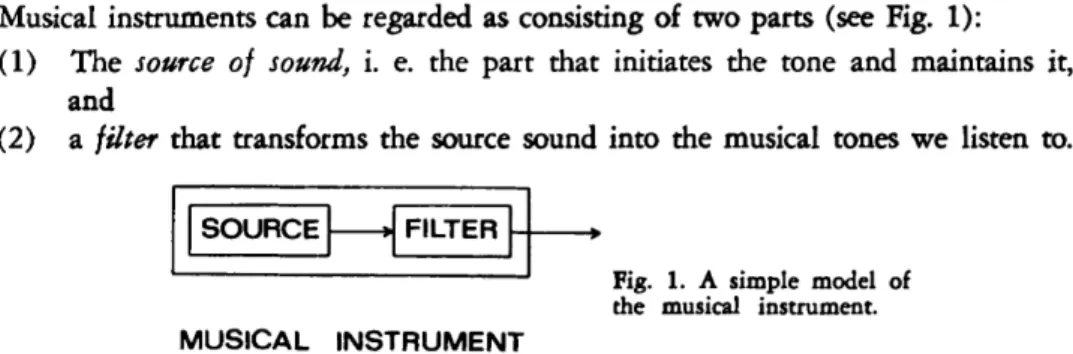
Musical instruments can be regarded as consisting of two parts (see Fig. 1):

(1)

(2)

The source of sound, i. e. the part that initiates the tone and maintains it, and

a filter that transforms the source sound into the musical tones we listen to. SOURCE FILTER

Fig. 1. A simple model of

the musical instrument.

MUSICAL INSTRUMENT

The model applies to the violin The string vibrations are the source and the sounding box is the filter.

This

means that the filter, i. e. the sounding box, is Invited lecture at the Second workshop on Physical and neuropsychologal foundations of

music, Ossiach, Austria, 1977. The paper has been edited for publication, but is otherwise unchanged.

(3)

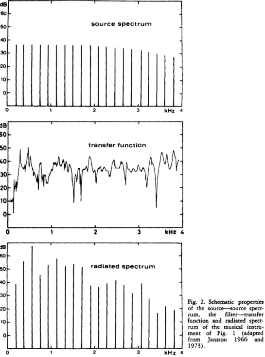
source spectrum

transfer function

radiated spectrum

Fig. 2. Schematic properties

of the source-source spect-

rum. the filter-transfer function and radiated spect-

rum of the musical instru-

ment of Fig. 1 (adapted from Jansson 1966 and 1973).

adjusted by the maker and cannot be changed by the player. The player, however, can adjust the source parameters in playing.

In Fig. 2, properties of the source, of the "sounding box filter", and of the radiated sound are sketched. In the diagrams the horizontal axis displays frequency in kHz and the vertical axis the amplitude, i. e. the strength, in

dB.

The upper diagram shows some basic source parameters of a violin tone. The diagram displays

20 vertical bars, i. e. the source contains a spectrum of 20 partials with somewhat decreasing strength. The frequency of the lowest partial corresponds closely to the pitch of the tone. Furthermore, there is noise in the source-the noise forms a band along a 0-dB line not drawn in the diagram.

The middle diagram displays properties of the sounding box, i. e. its trans- formation of the source spectrum. The transformation is determined by the amount of amplification by the sounding box. We can see that it varies considerably with frequency, including several peaks and dips. The amplification varies with increasing frequency irregularly and as much as 10 dB.

In the lowest diagram the

radiated

sound of the musical tone is sketched. We find the same number of bars, i. e. partials, as in the diagram of the source. The heights, the strengths of the partials, however, are quite different. The reason for this is that the different partials of the source (the upper diagram) are differently amplified by the filter. The amounts of amplification are given by the transfer function at corresponding frequencies (the middle diagram). As the transfer function is not constant, some partials are much amplified, others little, and we obtain musical tones with partials of very different strengths. Thus the different strengths of the radiated partials derive from the properties of the sounding box. The radiated spectrum of a musical tone equals the product of the source spectrum and the transfer function.

A

comparison of the source spectrum with the radiated spectrum in Fig. 2 shows that the maximum amplification of the sounding box is approximately 30

dB.

This

corresponds to the difference found by measuring the sound output from a violin played a) in normal condition and b) with the sounding box damped out (Jansson 1966).

The picture given so far is by no means complete. The upper diagram describes the source at one instant only. In real playing, the player changes the source spectrum continuously. First, of course, he can change the fundamental frequency of the played tones (by changing the free length of the string with his fingers. But even within the same tone the variations are considerable. The musical tones have attacks and ends where intensity and spectrum shape change with time. Furthermore, the player can influence both the strengths of the different partials and the noise level by varying bowing position, pressure, and speed. Finally, ex- periments prove that the bowed string does not vibrate with exactly constant frequency but with small variations superimposed (Cardozo and van Noorden 1968). The properties of the source can thus be summarized as follows: The source spectrum varies with time, it contains several partials of somewhat different strengths, noise, and a somewhat unsteady fundamental frequency.

Small amounts of the string vibrations leak through the bridge to the sounding box. The properties of the bridge have recently been investigated by Reinicke (1972). He found two prominent resonances of the bridge, the lower one at 3060

Hz.

This resonance gives maximum leakage of source partials around this frequency. This may be important for the tonal quality-the e a r has maximum sensitivity in this range and a singer can use this region to give his voice a specific timbre and carrying power.

(4)

Fig. 4. Transfer functions before and after varnishing (from Meinel 1937).

Fig. 3. Transfer functions with different plate thicknesses: a, thicker than n o r d , b, normal thickness and c, thinner than normal (from Meinel 1937).

Let

us now study the sounding box, the filter, and its transmission characteristics. We have already seen in Fig. 2 that the transfer function gives an amplification that varies greatly with frequency. Fig. 3 from Meinel (1937) shows how the violin maker can vary it.

As

before, we have the frequency along the horizontal axis marked by tonal positions, c1 being equal to 262

Hz,

and the strength of amplification with a linear scale along the vertical axis. The upper diagram de- rives from a violin with extra thick plates, the middle from one with plates of normal thickness, and the lowest from one with thin plates. A comparison of the three diagrams shows that the tallest peak is lowered in frequency, the peak- to-dip ratio increases, and the amplification at lower frequencies is increased by thinning the plates. The effects of the changes are substantial.

The varnish used by Stradivarius is often referred to as the key to the excellence of his instruments. The measurements by Meinel in Fig. 4 with a) full line before varnishing and b) 'broken line after varnishing show that this can hardly be the case. The influence of the varnish is small compared to the influence of variations in thickness of the plates. Furthermore, Meinel's measurements show that the

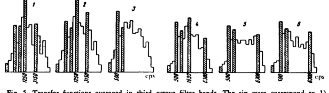
Fig. 5. Transfer functions averaged in third octave filter bands. The six cases correspond to 1)

classical mean, 2) bright, 3) noble, 4) nasal, 5) tight, and 6) constricted timbre (from Yankovskii 1966).

degree of arching, and the fitting and positioning of the sound post, influence the properties of the sounding box more than does the varnish.

It is very difficult to keep track of all resonances and the magnitude of amplification at all frequencies and compare the properties of sounding boxes of different violins in this way. Therefore, it is common to average the amplification over fairly broad frequency bands. The results are fairly sensitive to the way in which the averaging is made. Typical results from such measurements are given in Fig. 5, recorded by Yankovskii

(1966).

In this case the averaging has been made in third octave filter bands. The diagrams are plotted with a horizontal frequency scale and a linear strength amplification scale along the vertical axis. The diagrams show that in spite of the coarse averaging typical differences between different violins can be detected.

The properties of the sounding box can thus be summarized as follows: The sounding box works as an amplifier with an invariant but very complex amplification curve. The amplification curve is far from constant after averaging over broad frequency ranges In detail, it varies greatly with frequency, with many sharp peaks and dips.

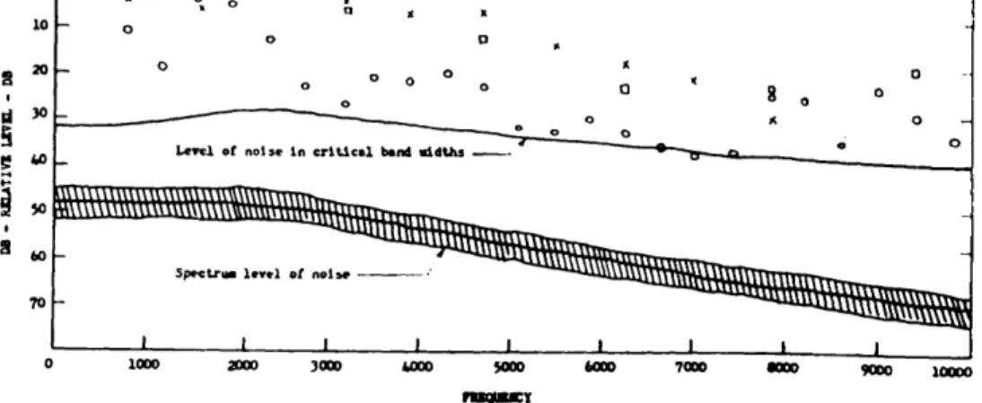
Records of radiated sound spectra by Fletcher, Blackham and Geertsen (1965) are shown in Fig. 6. The horizontal axis displays frequency in

Hz

and the vertical

axis strength in dB. The circles, crosses, and squares mark the strength amplitude

(5)

Fig. 6. Radiated sound spectra of violin tones. The circles mark partials of G3 (196 Hz), crosses

C4 (262 Hz), and squares G4 (392 Hz). The cross-hatched region marks spectrum level of noise, and the line marks noise level in critical band widths (from Fletcher, Blackham and Geertsen

1965). I

the tops of the bars in Fig. 2. By drawing imaginary lines between the circles, we can see that the strengths of the partials do indeed vary considerably with frequency. The same is true for the partials of the tones represented by crosses and squares. The measured spectrum level of noise is plotted as broad cross-hatched band. From this level the noise level in critical bandwidths has been calculated, i. e. the noise level we perceive with our hearing. This latter noise level is by no means negligible compared to the strength of partials in the high frequency range.

Fig. 7 from Fletcher and Sanders (1967) shows main parameters of "real" and "synthetic" radiated violin tones played with vibrato. The horizontal axis

displays time in all cases. The upper pair of diagrams displays the variations in fundamental frequency, with a vertical cent scale. The frequency variations are of the magnitude of 20 cents, i. e. one per cent in frequency, approximately. The next eleven pairs of diagrams show the variations in strength along the vertical axis for the total spectrum and the first ten partials. It is easily seen that the different partials vary differently in strength with time. Some partials vary little-the first and the fourth, for instance. Some vary much-the third and the seventh, for instance. A detailed study shows that the variations are not in phase with the frequency variations in all cases. In some cases the strength of a partial increases with increasing frequency while another partial may decrease in strength.

The result of the analysis of radiated violin tones by Fletcher and co-workers was summarized as follows: "The characteristics, essential to describing a tone, are the harmonic structure of the middle portion of the tone fand] the harmonic structure of the ending of the tone" and "The intensity level varies at 'the rate of the vibrato' but is greatly different for each harmonic of the same note. The

Fig. 7. Real and synthetic radiated sound spectra of violin tones played with vibrato. Frequency level vibrato (top line) and intensity curves for the total tone and first ten harmonics for G4

(6)

amplitude of harmonics’ not only vary in amplitude but differ in phase”.

. .

”There is a group of tones that do not come from the bowed string but from the open strings.”.

.

”They have an important effect upon the quality of the tone from the violin only when any of their natural frequencies are near those of the tones from the bowed string. These tones are an important part of the afterring. Finally, the bowing noise affects the quality of the tones, particularly those produced by the A and E strings.”

Perception

of

violin tones

Let us turn to the perceived quality of violin tones. Although more work is still needed for breaking the acoustical code of what determines the quality, we can draw some general conclusions. Some properties of the sounding box can be summarized in amplification levels averaged over broad frequency bands. Similar averaging has also been applied to studies of the radiated sound and its relations

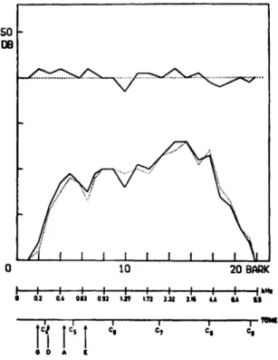
to perceived tonal quality. Let me as an example take an investigation by Gabriels- son and Jansson (1977). The violin radiates differently in different directions. To eliminate this difficulty, the recordings were made in a reverberation chamber. Scales were played on twenty quality-rated violins and recorded on tape. After- wards the average spectra of the scales were plotted, i. e. the long-time-average- spectra

(LTAS)

of the played scales.

As most of the remaining figures are drawn as Fig. 8, I shall explain it in some detail. The vertical axis displays strength along an ordinary

dB

scale. The horizontal axis displays frequency with a Bark scale.2 In this particular figure, two

additional frequency scales have been plotted. The lowest scale below the

Bark

scale marks the corresponding musical tones, G, D, A, and E being the frequencies of the open violin strings. The middle scale marks the frequencies corresponding to the Bark numbers. Analysis with filters one Bark wide has proved in many experiments to be a good approximation of the function of our hearing, for instance in the evaluation of loudness.

In the lower part of the diagrams two spectra are plotted and in the upper part the deviations between these spectra. In Fig. 8, two groups of long-time- average-spectra are plotted, the long-time-average-spectra of the eight violins rated highest (full line) and those of the seven rated lowest (dotted line). The diagram shows that the deviations are small, generally 2

dB. This

result has typically been found in most investigations-the average deviations between different groups of instruments are small. A natural interpretation is that several factors are important and few instruments score high in all. The small deviations, however, seem valid to describe some tonal qualities. A correlation coefficient of 0.8 was

1 Read: “The harmonics do not...”

2 _{One Bark equals one critical band of hearing (Frequenzgruppe),}_see_Zwicker,_E._&_Feldt-

keller, R.: Das Ohr als Nachrichtenempfänger, Stuttgart 2/1967. The ear has 24 critical bands of hearing spaced one Bark apart and thus forming a scale from O to 24 Bark. The Bark scale is approximately linear up to 1 kHz and thereafter logarithmic (for ready reference it may be noted that 10 Bark is approx. 1 kHz, 15 Bark is 3 kHz, and 20 Bark is 6 kHz).

Fig. 8. Long-time-average-spectra. Lower part: LTAS

of eight violins with high (-) and LTAS of

seven violins with low tonal quality ratings ( . . . . ) . Upper part: Difference between the two LTAS. The Bark frequency scale is defined in relation to the kHz frequency scale and equally tempered tone- scale with G, D, A and E being the open strings

of the violin (from Gabrielsson and Jansson 1977).

obtained between the tonal quality ratings from the playing tests and quality scores calculated with the difference function. Thus, we may conclude that strong frequency components are favourable at low and medium high frequencies, while weak frequency components are favourable at 10 Bark and high frequencies.

To the data collected factor analysis was also applied. The result is given in Fig.

9,

in which the factor loadings of a five factor solution are drawn. The solution accounts for 74 % of the variance of the long-time-average-spectra. Major areas of factor loadings are shaded. The first three factors in particular seem significant. The first factor says that strong frequency components at low frequencies are favourable, and the second factor that weak frequency components at high frequencies are favourable. The third factor says that strong frequency com- ponents beetween 10 and 14

Bark

are favourable. The result is similar to that of the difference function but more clearly marked.

Previously I showed that average differences between groups of instruments are generally small. The deviations between individual instruments, however, may be considerable. Fig. 10 shows that the difference between these two violins is especially large (as marked by the shaded areas) for the third factor, F 3. This

(7)

Fig. 10. Example of extremes for factor F3, maximum factor score (-), minimum factor score ( . . . . ) . Shaded parts indicate factor loadings 0.50 as given in Fig. 9 (from Gabrielsson and Jansson 1977). ,

Fig. 9. Graphical display of factor loadings within each of the factors 1-5 (vertical) for different filter bands (horizontal axis). The curve for each factor represents the size and sign (positive or negative) of the factor loadings for different filter bands. Shaded parts indicate factor loadings 20.50 (positive or negative) (from Gabrielsson and Jans- son 1977).

supports the previous interpretation that coarse averaging may suppress important deviations. A final remark from this investigation should be made. By comparing factor scores of the twenty quality-rated violins with factor scores of two more precious instruments, it was revealed that the factor scores of the precious instruments were, with few exceptions, within the ranges of the less precious instruments. This suggests, in contradiction to the previous interpretation, that the best instruments are obtained by a balance between different factors and not

by

a maximum score in some and minimum in others.

In the following, the perceptual importance of "suspected" parameters shall be

discussed.3

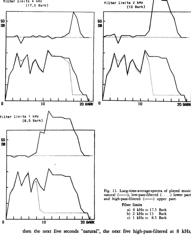
I feel that by now we have reached the stage where this really can be done by systematically varied synthesis. By doing so we may be able to eliminate factors of no importance and even pin down the relative importance of others.

Let us start with a simple experiment to provide some feeling for the impor- tance of different frequency regions. Sound example l u consists of 25 seconds of music, the first five seconds "natural", the next five low-pass-filtered at 8 kHz,

T h e sound examples are to be found on the record accompanying this issue of the journal. 3

Fig. 11. Laag-time-average-spectra of played music, natural (-), low-pass-filtered ( . . . . ) lower part,

and high-pass-filtered (-) upper part. Filter limits

a) 4 kHz = 17.5 Bark

b) 2 kHz = 13 Bark c) 1 kHz = 8.5 Bark

then the next five seconds "natural", the next five high-pass-filtered at 8

kHz,

and finally the last five seconds "natural"."

I think that many will hear the difference between the natural and the low- pass-filtered music, but they will agree that the difference is small. Furthermore, I think it will be agreed that little sound is left above 8 kHz.

(8)

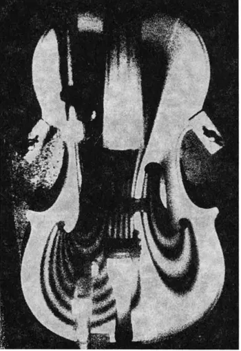
Fig. 12a. Interferogram of a violin, showing the vibrations of

the first top plate resonance with equal amplitude lines. These lines show that the plate

vibrates mainly in its left pan and that the sound post imposes a nodal line (from Jansson, Mo- lin, and Sundin, in Jansson

1977).

These conclusions are natural if we look at the longtime-average-spectrum of the music (Fig. 11a, the full line). The frequency limit of 8

k H z

equals 21 Bark, a frequency above which no sound is recorded in the spectrogram. Let us repeat the experiment with a filter limit of 4

kHz,

i. e.

17.

5 Bark, thus splicing up the sound as marked in Fig. 11a. The full line in the lower part corresponds to natural and the dotted to Iow-pass-filtered music. The full line of the upper part indicates the high-pass-filtered music. The order in the next sound example is natural, low- pass-filtered, natural, high-pass-filtered, and natural. (Sound example 1b.) I think it will be agreed that the influence of the region above 4 kHz is easily heard both in the low-pass and high-pass-filtered music but still moderate.

Let us repeat the process with the high-pass and low-pass filterings at 2 kHz, Fig. 1 1b (sound example I c), and finally at 1 kHz, Fig. 1 1c (sound example I d).

As

a conclusion from this little experiment, I do think we found that the tonal quality is influenced by the level in broad frequency bands, little for frequencies above 8 kHz, considerably for frequencies between 4 and 8 kHz but mainly for frequencies below 4

kHz.

Fig. 12b. The traditional and the new violin family (upper and middle parts respectively). T h e lower part shows the geometrical measures of the different instruments (from Hutchins and Bram

(9)

Fig. 14. Long-time-average- spectra of sound examples 2a ( . . . . ) and 2b (-).

Fig. 13. Peak-to-valley curves for various Q's of electronically simulated resonances

at Stradivarius peaks (from Mathews and Kohut 1973).

Some synthesis experiments have already been made along the suggested lines. One very successful synthesis of real instruments has been made

by

Saunders, Schelleng, and Hutchins in close cooperation. Saunders

(1953)

found experimen- tally that two resonances of the violin should be the most important. The first is the main wood resonance, which to a large extent consists of the first top plate resonance as shown in Fig.

12a.

The top plate vibrates mainly in phase a t t h i s resonance, thus giving a strong coupling to the lowest resonance of the enclosed air volume. Thereby, an additional resonance is obtained in the violin. The two resonances should be close to the frequencies of the middle open string to give a strong and even frequency response. With this in mind Schelleng

(1963)

has calculated design rules for the scaling of the instruments of the violin family. Hutchins

(1967),

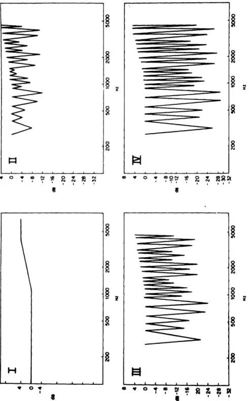
finally, has constructed and built a new family of violin instruments, following the scaling rules, see Fig. 12b.

This

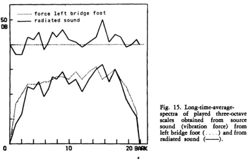
violin family consists of eight members, from a large bass to a small violin tuned an octave above the ordinary violin. The lowest part of Fig. 12b shows the dimensions chosen for the new instruments In order to make them playable and to make it possible to test their qualities, they must also be scaled to the size of the human body. The instruments are successful; the cello, for instance, has lost its notorious wolf note. By this synthesis, the importance of a well balanced low frequency range for violin tones has been proved.

But what about the influence of the detailed frequency function with a large number of peaks and dips? Experiments with such transfer functions have been made by Mathews and Kohut (1973). They picked up electromagnetically the string vibrations at the bridge of a violin without a sounding box. The source sound thus obtained was fed through an electronic filter bank with a large number of filters. The filters were arranged to approximate the transfer function cf the

(10)

Fig. 15. Long-time-average- spectra of played three-octave

scales obtained from source

sound (vibration force) from left bridge foot (....) and from radiated sound (-).

.

PLAYER SOURCE FILTER ROOM

sound

example 2, a scale is played three times in succession, first with a transfer function as in diagram I (2a), the second time as in diagram II (2b), and finally according to diagram IV (2c). I think everyone will hear a not very natural violin sound in the first scale, a considerably more natural one in the second, and a hollow violin sound in the last scale.

The synthesized violin tones may seem very unnatural, but compare sound example

2d,

a short piece of music for two violins. One part is played by the

"synthetic" violin and the other by an ordinary violin. In my opinion it is not so easy to say which instrument is which.

From this we can conclude that neither a smooth nor a very wiggly transfer function is favourable, i. e. the transfer function of the sounding box should have some wiggliness but not too much.

Fig. 14 displays the long-time-average-spectra of the first and of the best synthesis in the previous sound examples. The synthesized transfer functions have

a very smooth level, averaged over frequency bands 1 Bark wide.

This

is contradic- tory to the transfer functions presented by Yankovskii, for instance, and the long-time-average-spectra presented for real violins.

Recently I tried a simple synthesis experiment

A

piezoelectrical crystal was glued into the left bridge foot of my violin. Thus, the force excerted on the rop plate

by

the string vibrations could be recorded. Corresponding long-time-average- spectra of this force and the radiated sound are shown in Fig. 15. A filter bank, MARS5 similar to that of Mathews and Kohut, was used for the synthesis. It was set to give a rough approximation of the resonances of a violin.

6 _{MARS (Music Analog Resonator System)}_is_{a filter bank similar}_to_that_{of Mathews and} Kohut. in its first assembly the "hum" was too high, which unfortunately could not be filtered out in sound example 3.

LISTENER Fig. 16. Long-time-average

spectra of three-octave scales a) played through electronically simulated transfer function (with MARS) with the source sound of Fig. 15 ( . . . . ) and b) the

radiated sound of the real violin of Fig. 15 (-).

(11)

Fig. 18. Long-time-average- spectra of played scales recorded in the left ear (-) and right ear ( . . . . ) of the player and one

ear of the listener (----).

ding spectrum for a listener in the room a few meters away is also included. Compared to the player’s right ear,

his

left gets a considerably higher level with a high frequency pre-emphasis The listener obtains something in between. When

this

is replayed stereophonically over headphones, one has the sensation of playing oneself. The difference in signal between the ears, however, is so great that a non-violin-player spontaneously remarked that there was no sound in his right earphone. To give an idea of the difference, the sound to the left ear and the right ear are replayed in succession in

sound

example

4.

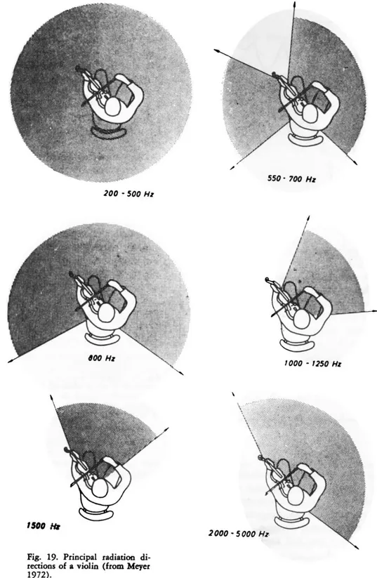
In the recordings the influence of the acoustics of the room may be noticed in the position of the ears of the player.

The violin is a sound source

with

a complex directional characteristic, as shown by Meyer (1972), Fig.

19. As

a rule, the violin radiates more or less omnidirectionally at low frequencies, but with rising frequency the directional characteristics become more and more complex.

Let us look at long-time-average-spectra corresponding to four directions of the violin and player. In Fig. 20a we see the long-time-average-spectra obtained in the directions marked by the arrows on the top of the violin in the upper left corner. Direction b (the full line) gives stronger high frequency components than direction a (dotted line). The two long-time-average-spectra in Fig. 20b show that the new direction b (full line) gives an overall much lower level than the reference direction a – t h e same reference direction as in the previous figure (dotted line). The last pair, Fig. 20c, shows that in the third new direction b (full line) the overall level and the level for frequencies above 10 Bark are lower than for the reference direction a (dotted line). It may be observed that in this

third pair we have the directions of first and second violins in one type of orchestral arrangements. A soloist should aim at his listeners with the scroll to

Fig. 19. Principal radiation di- rections of a violin (from Meyer

(12)

Fig. 20. Long-time-average- spectra of a violin obtained in

an anechoic chamber in four directions according to sketch

in upper left corner.

penetrate through the orchestral accompaniment whereas a second violinist may be disfavoured in brilliance compared to his fellow first violinists. The three pairs of long-time-average-spectra may be compared with recordings in the same directions in an anechoic chamber. (Sound examples 5a, b and c.) Five seconds in the reference direction a (the dotted line) are followed by five seconds in direction b (the full line). The same procedure is repeated for all three different directions b.

The above recordings were made in a very heavily damped room, that is,

a room with no reverberation. Let me finish by demonstrating how bowed string instruments sound in a room with much reverberation- reverberation cham-

Fig. 21. Long-time-average-spectra of a scale and a piece of music played on the violino grande (from Jansson 197 7 ) .

ber. The long-time-average-spectra of Fig. 21 (Jansson 1977) show that the spectrum level is moderately influenced by the combination of reverberation and music. In one of the spectra a scale was played and in the other a piece of music. In the example we first hear two violins in succession (sound example 6a) and then the music excerpt (6b). I think it will be agreed that the quality impres- sion is much influenced by the room acoustics. It is hard to hear quality differences between the two different instruments cf. Fig. 10. But in the case of the excerpt from an actual composition and room acoustics with long reverberation, the distortion on the music is small. The music may have been composed to fit the

condition of a long reverberation time. The acoustics of ordinary rooms fall in-between the extremes demonstrated here.

Conclusion

In this schematic and by no means complete review I have shown that mnal characteristics of the violin are determined by the source, the bowed string, and that the sound of this source is amplified by the sounding box. The source is made up of time-variant spectra, which are amplified by the sounding box in a complex way. Both the strength of the partials and the amplitude modulation of the partials seem important to the perception. Furthermore, I have shown that a player and a listener receive quite different tones. Differences in directions are easily heard in a heavily damped room, and average-level deviations in broad frequency bands between instruments can be transmitted through very reverberant rooms. Both the player and the room should be regarded as extensions of the musical instrument.

(13)

Acknowledgements:

Helpful discussions with and the performance of the sound examples by Bronislaw Eichenholz and Lars Frydén are gratefully acknowledged. Mrs. Carleen Hutchins has kindly supplied Fig. 12b.

Sound examples

Track I. From J. S. Bach: Brandenburg concerto no. 3, G major, BWV 1048 (2’).

l a ) Normal, low pass 8 kHz, normal, high pass 8 kHz, normal

b) 4 4

c) 9, 9, 2 2

d) 1 1

Cf. Fig. 1 1.

Track II. Mathews and Kohut: Electronic violin with adjustable resonances (1’40”). 2a) Scale with Q-values adjusted according to Fig. 13:I

b) ,, Fig. 13:II

c) ,, Fig. 13:IV

d) From B. Bartók: 44 Duos für zwei Violinen (1931), no. 14, A minor, with an electronic violin and an acoustic violin.

Track III. A simple synthesis experiment (55”).

3a) Source sound (vibration force under left foot of bridge) b) Synthesized radiated sound

c) Natural radiated sound Cf. Fig. 16.

Track IV. From J. F. Mazas: Douze petits duos pour deux violons.

Op. 38, no. 3, D major (30”).

4a) Recording in the left ear of the player

b) right

Cf. Fig. 18.

Track V. Excerpts from recordings in four different directions of a violin in an anechoic chamber (40”).

5a) The microphone to the right of the player and in front of the player.

b) behind the player.

C) ,,

,,

to the left of the player.

Cf. Fig. 20.

Track VI. Excerpts from recordings in a reverberation chamber (35”).

6a) A scale on two violins

b) From J. S. Bach: Sarabande from Suite no. 6 for violoncello solo, D major,

BWV 1012, played by B. Eichenholz on a violino grande.

References

Cardozo, B. L. and van Noorden, L. P. A. S.

(1968): Imperfect periodicity in the

bowed string. (3rd Annual progress report, Inst. v. Perceptie Onderzoek, Eind- hoven, pp. 23-28.)

Fletcher, H. and Sanders, L. C. (1967): Qua-

lity of violin vibrato tones. (J. Acoust. Soc.Am. 41, pp. 1534-1544.)

Fletcher, H., Blackham, E. D. and Geertsen,

O. N. (1965): Quality of violin, viola,

’cello, and bass-viol tones. I. (J. Acoust. Soc.Am. 37, pp. 851-863.)

Gabrielsson, A. and Jansson, E. V. (1977):

Long-time-average-spectra and rated quali-

ties of twentytwo violins, submitted for

publication in Acustica; preliminary re-

port in An analysis of

long-time-average-spectra of twentytwo quality-rated violins.

(Speech Transmission Laboratory, Quarterly progress and status report, 1976/2

-3, pp. 20-34, KTH, Stockholm.)

Hutchins, C. M. (1967): Founding a family

of fiddles. (Physics today 20, no. 2, pp. 27-38.)

Hutchins, C. M. (1975 and 1976) (ed.):

Musical acoustics. Part I: Violin family components. Part II: Violin family functions. Dowden, Hutchinson & Ross, Inc., Stroudsburg, Pennsylvania. (Benchmark papers in acoustics, 5-6.)

Hutchins, C. M. and Bram, M. (1973): The

bowed strings, yesterday, today, and to- morrow. (Music Educators J., Nov.) Jansson, E. (1966): Analogies between

bowed string instruments and the human voice, source-filter models. (Speech Trans- mission Laboratory, Quarterly progress and status report, 1966/3, pp. 4 - 6 ,

KTH, Stockholm.)

Jansson, E. (1973): Om undersökningar av

fioler. (Svensk naturvetenskap, pp. 173- 180, Statens naturvetenskapliga forsk-

ningsråd, Stockholm.)

Jansson, E. (1977): On the acoustics of mu-

sical instruments. (Music, room and acoustics, pp. 82-113, Royal Swedish Academy of Music, Stockholm.)

Jansson, E., Molin, N-E. and Sundin, H.

(1970): Resonances of a violin body stu-

died by hologram interferometry and acoustical methods. (Physica scripta 2, pp. 243-256.)

Mathews, M. V. and Kohut, J. (1973):

Electronic simulation of violin resonances. (J. Acoust. Soc.Am. 53, pp. 1620-1626.)

Meinel, H. (1937): Über Frequenzkurven von Geigen. (Akust. Z. 2, Jan., pp. 22-

3 3.)

Meyer, J. (1972): Directivity of the bowed

stringed instruments and its effect on orchestral sound in concert halls. (J. Acoust.

Soc.Am. 51, pp. 1994-2009.)

Reinicke, W. (1972): Die Übertragungsei-

genschaften des Streichinstrumentensteges, Dissertation, Technische Universität, Ber- lin.

Saunders, F. A. (1953): Recent work on violins. (J. Acoust. Soc.Am. 25, pp. 491- 498.)

Schelleng, J. C (1963): The violin as a circuit. (J. Acoust. Soc.Am. 35, pp. 326- 338 and p. 1291.)

Yankovskii, B. A. (1966): Methods for the

objective appraisal of violin tone quality. (Soviet physics acoustics 1 1 , pp. 231- 245.)