The solar Mg abundance from strong
spectral lines in the infrared
Khaled Al Moulla
Supervisor Paul S. Barklem
Master Programme in Physics: Astronomy and Space Physics Advanced Physics – Project Course (1FA565)
λ10811 and λ10965. Downloaded line data from VALD are updated with modern values for the oscillator strengths and van der Waals damping parameters, the latter obtained through ABO theory. Utilizing SME, the Mg abundances of synthetic spectra are fitted with respect to a solar atlas. The derived abundance for varied turbulence configurations is found to be between log AMg + 12 = 7.40–7.52, which is slightly lower than meteoric and 3D-modeled
values. Suggested improvements would be to consider the effects of NLTE and line blending. Key words. Sun: Mg abundance – line broadening: ABO theory – VALD – SME
Contents
1 Introduction 1 2 Theory 1 2.1 Line formation . . . 1 2.2 Collisional broadening . . . 2 2.2.1 Unsöld theory . . . 2 2.2.2 ABO theory . . . 2 2.3 Curve of growth. . . 3 3 Methods 3 3.1 Line data . . . 3 3.1.1 MgIλ10811 . . . 3 3.1.2 MgIλ10965 . . . 4 3.2 Spectral synthesis. . . 4 4 Results 4 4.1 Line width comparison . . . 44.2 Mg abundance . . . 5
5 Discussion 5 5.1 Comparison with other works . . . 5
5.2 Possible improvements . . . 6
6 Conclusion 6 References 7 A Derivation of the Unsöld (1955) formula 8 B VALD queries 10 B.1 Line data for the interval around MgI λ10811 . . . 10
1
Introduction
The synthesis of stellar spectra can be notori-ously difficult because of the necessity to ac-count for numerous parameters and processes. The purpose of this project is to determine the magnesium (Mg) abundance in the Sun, by appropriately updating the atomic properties of two infrared Mg lines, using state-of-the-art theories and measurements.
In Sect. 2, the basics of line formation and the inadequacies of old models are explained. In Sect. 3, the selected spectral lines as well as the utilized software and online services are described. InSect. 4, the line widths and abun-dances derived from varied procedures are pre-sented, and thereafter discussed along with pos-sible improvements inSect. 5.
2
Theory
Unless otherwise stated, the following equations are all expressed in the centimeter-gram-second (cgs) unit system.
2.1 Line formation
The process of line absorption is classically de-scribed as the interaction between a plane tromagnetic wave and a bound oscillating elec-tron which, together with its nucleus, acts as an electric dipole (Mihalas 1970). The average power from the obstructed wave is
hP i = ανcE
2 0
8π , (2.1)
where E0 is the electric field amplitude and
αν the absorption coefficient per frequency ν,
whereas the radiated power from a point charge moving with velocity v is estimated by
P ≈ 2 3
e2v92
c3 . (2.2)
Solving the equation of motion for a harmonic oscillator,
m(:x + ω20x) = eE0eiωt− 2mγ 9x , (2.3)
where ω0 and ω are the angular frequencies of
the undamped motion and the driving wave, respectively, and γ is the damping parameter,
allows the rewriting and averaging ofEq. (2.2),
hP i ≈ e 4ω4 3m2c3 E02 (ω2− ω2 0)2+ 4ω2γ2 . (2.4)
EquatingEqs. (2.1)and (2.4), and making the appropriate approximations, the absorption co-efficient can be expressed as
αν ≈ 2 πe2 mc γ (ω − ω0)2+ γ2 . (2.5)
Integrating over all frequencies, and substitut-ing x ≡ ω − ω0, αtot = Z ∞ 0 αν dν ≈ πe2 mc Z ∞ −∞ 1 π γ x2+ γ2 dx , (2.6) the last integrand is identified as a normalized Lorentz dispersion profile with half-width at half-maximum (HWHM) γ. In other words, the line absorption profile is naturally broad-ened. However, a quantum mechanical treat-ment finds that the total absorption is overesti-mated, leading to the introduction of a dimen-sionless factor, the oscillator strength f,
αtot =
πe2
mcf , (2.7)
which is unique for each transition and can be related to the Einstein coefficients. It is com-monly given in the form log gf, where g is the statistical weight.
Spectral lines are prone to other types of broadening, among them collisional (see
Sect. 2.2) and thermal, of which the former also produces Lorentzian distributions and the lat-ter Gaussian, leading to the final profile being a convolution between the two, known as a Voigt profile. Additionally, turbulence at different scales—micro- and macroscopic—induces fur-ther broadening.
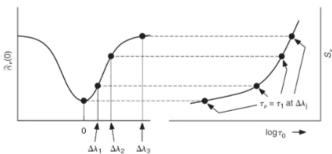
Another important aspect is the depth of for-mation. When mapping the surface flux Fν(0)
from the source function Sν(τ ), which specifies
the ratio of emission to absorption as a function of optical depth τ, the Eddington approxima-tion shows (Fig. 2.1) that the line core is formed near the surface of stellar photospheres, while the wings originate deeper inside (Gray 2005).
2
Figure 2.1 The mapping between the surface flux across a spectral line (left) and source function (right) reveals that the core is formed in more shal-low layers of the photosphere, i.e. smaller τ , than the wings. Credit: D. F. Gray 2005 (reproduced with permission).
2.2 Collisional broadening
Collisional (or pressure) broadening is a collec-tive term for several types of interactions be-tween atoms and perturbers. In this work, fo-cus will be on van der Waals broadening for which the perturbation is caused by neutral hy-drogen (H), common in cool, solar-type stars.
2.2.1 Unsöld theory
(See Appendix A for an extended derivation.) In the formulation by Unsöld (1955), the atom is described as a radiating oscillator experienc-ing a phase shift when passed by a perturber. The encounters are assumed to occur one at the time, and instantaneously compared to the intervals in-between (which is why this theory is commonly known as the impact approxima-tion). In terms of the mean time t0 between
collisions, the averaged and normalized energy spectrum is given by E(ω) = 1 π 1/t0 (ω − ω0)2+ (1/t0)2 , (2.8)
where γ = 1/t0 is recognized as the HWHM. It
is then customary to define an effective impact parameter ρ0, corresponding to the circular
ra-dius required to sweep out a volume in which one collision takes place every t0,
γ = Npπρ20hvi , (2.9)
where Np is the perturber number density and
hvi the mean relative velocity.
The change in angular frequency is assumed to follow a power law of the form
∆ω = Cn
rn , (2.10)
where Cn is an interaction constant, and n = 6
for van der Waals interaction. The total phase shift is then
φ =
Z ∞
0
∆ω dt , (2.11)
sometimes arbitrarily set to 1 rad, however, a more detailed analysis by Lindholm (1945) finds that an improvement is made if φ ≈ 0.61. Solving for ρ0 and plugging in n = 6, the
half-width per H atom becomes γ6 NH = πˆ 3π 8 C6 φ ˙2/5 hvi3/5 . (2.12) What remains is to compute C6, which is
done with the azimuthal and principal quan-tum numbers, the latter given by
n∗= d
RH
I − χ, (2.13)
where RH is the Rydberg constant for
hydro-gen, and I and χ are the ionization and excita-tion energies, respectively.
Consequently, these drastic simplifications have led to disagreement with experimental data, often requiring the line widths to be en-hanced with a factor of Á 2.
2.2.2 ABO theory
The successful approach by Anstee-Barklem-O’Mara (see e.g. Barklem, Anstee & O’Mara 1998), commonly referred to as ABO theory, has sought to improve the theoretical calcula-tions of collisional broadening due to neutral hydrogen. In short, second-order perturbation theory is applied to the interatomic interac-tion, allowing the evaluation of the scattering cross-section σ(v) for some perturber velocity v. Given the observed power-law dependence on v for the cross-section,
σ(v) = σ(v0)
ˆ v v0
˙−α
, (2.14)
where α is called the velocity parameter, and v0 = 10 km/s is a conventional reference value,
σ(v0)and α are calculated for different types of
transitions and tabulated against the effective principal quantum numbers of the lower and
upper state. These can then be converted into a half-width per H atom using
γ6 NH =ˆ 4 π ˙α/2 Γˆ 4 − α 2 ˙ ˆ hvi v0 ˙1−α v0σ(v0) , (2.15) where Γ is the Gamma function.
2.3 Curve of growth
The classification of line strengths is somewhat ambiguous. One suggested system can be de-fined from the curve of growth (Gray 2005), i.e. a logarithmic plot of the equivalent width W (the area enclosed by a spectral line) as a function of the chemical abundance AX =
NX/NH for some element X. In Fig. 2.2, it
is demonstrated how the behavior experiences three regimes. When W ∝ A, the line is classed as weak; as the central flux approaches its mini-mum value the line is said to be reaching satura-tion; and thereafter, for strong lines W ∝?A.
Figure 2.2 The equivalent width per wavelength (above) and relative flux (below) for varied absorber abundance. The circles indicate the different line profiles. Credit: D. F. Gray 2005(reproduced with permission).
3
Methods
3.1 Line data
The two studied spectral lines are MgIλ10811 and λ10965. Their line data is retrieved from the Vienna Atomic Line Database1 (VALD);
see Appendix B for the respective queries. The effective principal quantum numbers are calculated using Eq. (2.13) with multiplet-averaged energies obtained from NIST2, and
subsequently used to interpolate values for the ABO parameters. In each downloaded line list, the following adjustments are made:
• The Mg components of interest are iso-lated; the rest is deleted.
• The oscillator strengths are replaced, wherever possible, with updated values by
Pehlivan Rhodin et al. (2017, abbreviated asPR17).
• The van der Waals damping parameters are replaced with corresponding ABO val-ues. The accepted format is log (2γ6/NH)
or INT[σ(v0)] + α, where σ(v0)is in atomic
units (au) and INT rounds its argument to the closest integer, which is practical since σ(v0) > 1 au and 0 < α < 1.
3.1.1 MgI λ10811
The MgIλ10811 line is a d–f transition, consist-ing of six fine structure components (Table 3.1). Its ABO parameters, interpolated from the ta-bles in Barklem, O’Mara & Ross (1998), are found to be INT[σ(v0)] + α = 2982.335.
Table 3.1 MgI λ10811 componental wavelengths and oscillator strengths.
λ(Å) log gf log gf 10811. NIST PR17 .053 0.024 0.052 ± 0.04 .076 −0.137 .097 −1.038 .122 −1.036 .143 −2.587 .158 −0.305 −0.321 ± 0.04 1Available athttp://vald.astro.uu.se. 2 Available at https://www.nist.gov/pml/ atomic-spectra-database.
4
The left wing is blended with an uniden-tified neighbor. Therefore, a fake iron (Fe) line is constructed, with approximate proper-ties found through trial and error (seeTable 3.2
and Fig. 3.1), and added to the line list. Table 3.2 Fake Fe line.
Species FeI
Wavelength λ 10810.786Å
Excitation energy χ 1.0eV
Oscillator strength log gf −4.5 van der Waals damping
INT[σ(v0)] + α 1500.250
Figure 3.1 Above: Synthesis without fake Fe line. Below: Synthesis with fake Fe line.
3.1.2 MgI λ10965
The MgI λ10965 line is a p–d transition,
con-sisting of three fine structure components ( Ta-ble 3.3). The ABO parameters of such tran-sitions can be interpolated from the tables in
Barklem & O’Mara (1997), however, this line is off-table. Thus, its parameters, provided by the supervisor of this project from specific cal-culations, are INT[σ(v0)] + α = 3328.238.
Table 3.3 MgI λ10965 componental wavelengths and oscillator strengths.
λ(Å) log gf log gf 10965. NIST PR17 .386 −2.164 −2.184 .414 −0.989 −1.008 .450 −0.240 −0.260 3.2 Spectral synthesis
Syntheses are performed with Spectroscopy Made Easy3 (SME; Valenti & Piskunov 1996)
ver. 423, which implements the MARCS model atmosphere (Gustafsson et al. 2008) under local thermodynamic equilibrium (LTE). The soft-ware allows fitting of various stellar param-eters with respect to an NSO atlas (Kurucz et al. 1984), and for both of the selected lines, the Mg (and Fe, in the case of MgI λ10811) abundance is fitted with respect to a segment extended ±5 Å around their respective central wavelengths.
In order to avoid the disturbance of other lines, a mask is applied to each wavelength in-terval (see Fig. 3.2). The solar parameters in
Table 3.4are constant, whereas the turbulence velocity fields were initially considered to be free parameters alongside the abundance, how-ever, the unphysical outcome of test runs led to the decision that the micro- and macroturbu-lence should be fixed and incrementally varied. Table 3.4 Solar parameters.
Effective temperature Teff 5777K
Surface gravity log g 4.44
Metallicity [M/H] 0.0
4
Results
4.1 Line width comparison
From Eqs. (2.12) and (2.15), respectively, the half-widths per hydrogen atom are calculated according to the Unsöld and ABO theories, at a reference temperature of T0 = 10, 000 K. These
are presented in Table 4.1, and a numerical
3
Available for download athttp://www.stsci.edu/ ~valenti/sme.html.
Figure 3.2 Masks for the wavelength intervals around the MgIλ10811 (above) and MgIλ10965 (below) lines. Data points considered as line and continuum segments are colored brown and yellow, respectively, whereas ignored points are blank. The enlarged dashed boxes demonstrate how the final synthesis (blue curve) compares to the solar atlas (black curve) for vmic= 1 km/s and vmac= 2 km/s.
comparison shows that the enhancement factor is consistent with the literature.
Table 4.1 HWHM per hydrogen atom, in units of rad s−1cm3, for the studied Mg lines. The last
row specifies the factors by which the Unsöld widths have to be multiplied to attain the ABO ones.
MgI λ10811 MgIλ10965 γ6/NH 3.600 × 10⁻⁸ 3.655 × 10⁻⁸ Unsöld γ6/NH 1.061 × 10⁻⁷ 1.235 × 10⁻⁷ ABO Enhancement 2.947 3.378 factor 4.2 Mg abundance
The Mg abundance is obtained with iterative χ2-minimization in SME. The microturbulence is varied between vmic = 0–2 km/s in steps of
∆vmic = 0.5 km/s, and likewise for the
macro-turbulence with vmac= 0–4 km/s and ∆vmac=
2 km/s. The software returns the abundances as log (NMg/Ntot), where Ntot is total number
density, which are then converted into the con-ventional form log AMg+ 12.
The results are presented in Fig. 4.1, show-ing that dependshow-ing on the chosen turbulence configuration, the Mg abundance varies be-tween 7.45–7.52 for MgI λ10811, with an addi-tional variation of ±0.026 dex due to the uncer-tainty in the oscillator strengths, and between 7.40–7.50 for MgI λ10965.
5
Discussion
5.1 Comparison with other works The results inFig. 4.1have relatively small vari-ation and indicate a systematic trend of smaller abundance for more turbulent activity, which is expected since the observed broadening must be due to the abundance and turbulence in var-ious proportions if the collisional damping is held fixed. The trend is only broken by the MgIλ10965 configuration with vmac= 4 km/s.
The validity of derived abundances has to be strengthened through a consistency with other sources. Regarding the solar chemical composi-tion, the means of confirmation are scarce, and mostly limited to the measurements of metals in meteorites or other theoretical models. Lodders et al.(2009) evaluates the solar Mg abundance to be 7.6 in CI chondrites, whereasScott et al.
simula-6
0.0
0.5
1.0
1.5
2.0
v
mic[km/s]
7.40
7.42
7.44
7.46
7.48
7.50
7.52
log
A
Mg+
1
2
Mg
I10811
Mg
I10965
v
mac[km/s]
0
2
4
Figure 4.1 Mg abundances for different micro- and macroturbulence configurations. The errorbar indi-cates the range when changing the oscillator strengths to their extremes for MgIλ10811 (seeTable 3.1). tion, with non-LTE (NLTE) corrections, of the
solar photosphere to recommend 7.59 ± 0.04. Although there might be a slight overlap be-tween the uncertainties of this result and the aforementioned 3D model, the agreement is only present for MgI λ10811 under the condi-tions of a turbulence-free photosphere, which seems highly unlikely.
5.2 Possible improvements
The discrepancy in abundance determination, caused by the noted difficulty to reproduce line shapes, is thought to be caused by several fac-tors. Primary reasons could be failures in mod-eling the line cores due to NLTE effects or improperly accounting for line blending (done with an adjacent fake line for MgIλ10811 and a mask for the leftward wing of MgI λ10965).
Furthermore, although the oscillator strengths are believed to have been improved, the up-dated values were relatively uncertain and un-available for all components of MgI λ10811. Possible overestimation of the broadening from ABO theory, or some other, unknown problem, are also not excluded.
Similar studies should be conducted with additional Mg lines to investigate potential trends; ideally in the farther infrared, which would require the access to an atlas beyond the current NSO solar atlas in SME.
6
Conclusion
The derived solar Mg abundance of 7.40–7.52, varying from the scales of turbulence, is in dis-agreement with meteoric and 3D-modeled val-ues. Improvements should be done to ensure NLTE, line blending and the quality of atomic parameters are negligible sources of error.
Acknowledgement
The author would like to thank Prof. Paul S. Barklem for his much appreciated supervision and support throughout this project, which has indeed been a pleasant learning experience filled with unexpected twists and turns.
References
Barklem, P. S., Anstee, S. D. & O’Mara, B. J. (1998), ‘Line Broadening Cross Sections for the Broadening of Transitions of Neutral Atoms by Collisions with Neutral Hydrogen’, Publ. Astron. Soc. Aust. 15(3), 336–8. Barklem, P. S. & O’Mara, B. J. (1997), ‘The
broadening of p–d and d–p transitions by col-lisions with neutral hydrogen atoms’, Mon. Not. R. Astron. Soc. 290(1), 102–6.
Barklem, P. S., O’Mara, B. J. & Ross, J. E. (1998), ‘The broadening of d–f and f–d transitions by collisions with neutral hy-drogen atoms’, Mon. Not. R. Astron. Soc. 296(4), 1057–60.
Gray, D. F. (2005), The Observation and Anal-ysis of Stellar Photospheres, 3rd edn, Cam-bridge University Press.
Gustafsson, B., Edvardsson, B., Eriksson, K., Jørgensen, U. G., Nordlund, . & Plez, B. (2008), ‘A grid of MARCS model atmo-spheres for late-type stars’, Astron. Astro-phys. 486(3), 951–70.
Kurucz, R. L., Furenlid, I., Brault, J. & Tester-man, L. (1984), Solar flux atlas from 296 to 1300 nm, National Solar Observatory. Lindholm, E. (1945), ‘Pressure Broadening
of Spectral Lines’, Ark. Mat. Astron. Fys. 32A(17).
Lodders, K., Palme, H. & Gail, H. P. (2009), Abundances of the elements in the Solar System, in J. E. Trümper, ed., ‘Landolt-Börnstein: New Series’, Vol. VI/4B, Springer, chapter 4.4, pp. 560–630.
Mihalas, D. (1970), Stellar Atmospheres, 1st
edn, W. H. Freeman.
Pehlivan Rhodin, A., Hartman, H., Nilsson, H. & Jönsson, P. (2017), ‘Experimental and the-oretical oscillator strengths of Mg I for accu-rate abundance analysis’, Astron. Astrophys. 598, A102.
Scott, P., Grevesse, N., Asplund, M., Sauval, A. J., Lind, K., Takeda, Y., Collet, R., Trampedach, R. & Hayek, W. (2015), ‘The
elemental composition of the Sun: I. The in-termediate mass elements Na to Ca’, Astron. Astrophys. 573, A25.
Unsöld, A. (1955), Physik der Sternatmo-sphären, Springer.
Valenti, J. A. & Piskunov, N. (1996), ‘Spec-troscopy made easy: A new tool for fitting observations with synthetic spectra’, Astron. Astrophys. Suppl. Ser. 118, 569–603.
8
A
Derivation of the
Unsöld
(
1955
) formula
Modeling the atom as a radiating oscillator with natural frequency ω0, it will emit wave packets
of the form
f (t) = eiω0t. (A.1)
In the impact approximation, the phase change caused by a collision occurs at a much shorter time scale compared to the time in-between collisions tcoll. The Fourier transform of the wave
packets becomes, F (ω) = Z tcoll 0 f (t)e−iωt dt = e i(ω−ω0)tcoll− 1 i(ω − ω0) . (A.2)
The radiated energy spectrum is proportional to F (ω)F∗(ω), where F∗(ω)is the complex
conju-gate of F (ω). However, to obtain the true spectrum, one must take into account the probability for a collision to occur after tcoll,
P (tcoll) =
e−tcoll/t0
t0
, (A.3)
where t0 is the mean time between collisions. The energy spectrum is then given by
E(ω) = A Z ∞ 0 F (ω)F∗(ω)P (tcoll) dtcoll= 1 π 1/t0 (ω − ω0)2+ (1/t0)2 , (A.4)
where A is a normalization constant, and γ = 1/t0 is recognized as the HWHM for the
distribu-tion. It is useful to define an effective impact parameter ρ0, such that one collision occurs every
t0 inside its swept-out volume,
1 = Npπρ20hvi t0 ⇒ γ = Npπρ20hvi , (A.5)
where Np is the perturber number density and
hvi = d
8kT
πµ (A.6)
the mean relative velocity at temperature T for a Maxwell-Boltzmann distribution, with µ = mamp/(ma+ mp) being the reduced mass of the atom and perturber. The change in angular
frequency is assumed to follow a power law,
∆ω = Cn
rn , (A.7)
where Cn is an interaction constant and r the atom-perturber distance. Placing the atom at
the origin of a Cartesian coordinate system and considering a perturber traveling in y-direction (see Fig. A.1), the impact parameter is given by ρ = r cos θ. The total phase shift can then be expressed as φ = Z ∞ 0 ∆ω dt = Cn Z ∞ 0 cosnθ ρn dt = Cn vρn−1 Z π/2 −π/2 cosn−2θ dθ , (A.8)
where the substitution y = r sin θ was made using v = dy/dt. The effective impact parameter can be solved for some cut-off on φ (see main text),
ρ0 = ˜ Cn vφ Z π/2 −π/2 cosn−2θ dθ ¸1/(n−1) . (A.9)
Plugging in n = 6 for van der Waals interaction, and looking up the integrand in Eq. (A.9) in any suitable mathematics handbook, it is now possible to rewriteEq. (A.5) as
γ6 = NHπ ˆ 3π 8 C6 φ ˙2/5 hvi3/5 . (A.10)
The only computation remaining is that of C6, provided by the Unsöld approximation,
C6= αHe2a20 ¯ h `hr 2 ui − hrl2i˘ , (A.11)
where αHis the polarizability of hydrogen, a0 the Bohr radius, and
hr2i = n
∗2
2Z2 `5n ∗2
+ 1 − 3l(l + 1)˘ (A.12)
the mean-square radius of the valence electron (subscripts ‘l’ and ‘u’ indicate the lower and upper levels of the transition) calculated from the azimuthal l and principal n∗ quantum numbers, the
latter given by
n∗= Z d
RH
I − χ, (A.13)
where Z is the net charge felt by the electron (+1 for neutrals), RH the Rydberg constant for
hydrogen, and I and χ are the ionization and excitation energies, respectively.
Figure A.1 Schematic image of a perturber passing the atom. Credit: D. F. Gray 2005(reproduced and adapted with permission).
10
B
VALD queries
B.1 Line data for the interval around MgI λ10811
begin request extract stellar default configuration short format 10806.0, 10816.0 0.001, 1.0 5777, 4.44 end request
B.2 Line data for the interval around MgI λ10965
begin request extract stellar default configuration short format 10960.0, 10970.0 0.001, 1.0 5777, 4.44 end request