A study of the preliminary National Forest Inventory in Georgia

(1)

Rahel Beil

Supervisor: Per-Magnus Ekö, SLU, Southern Swedish Forest Research Centre

A study of the preliminary

National Forest Inventory in Georgia

- with special emphasis on degraded

vs. non-degraded forest

Swedish University of Agricultural Sciences

Master Thesis no. 308

(2)

(3)

Swedish University of Agricultural Sciences

Master Thesis no. 308

Southern Swedish Forest Research Centre

Rahel Beil

Supervisor: Per-Magnus Ekö, SLU, Southern Swedish Forest Research Centre

Examiner: Eric Agestam, SLU, Southern Swedish Forest Research Centre

A study of the preliminary

National Forest Inventory in Georgia

- with special emphasis on degraded

(4)

A study of the preliminary National Forest Inventory in Georgia

- with special emphasis on degraded vs. non-degraded

forestsubtitle

Rahel Beil

Supervisor: Per-Magnus Ekö, SLU, Southern Swedish Forest Research Centre Examiner: Eric Agestam, SLU, Southern Swedish Forest Research Centre

Credits: 30 credits

Level: Advanced Level (A2E)

Course title: Master thesis in Forest Management

Course code: EX0838

Programme/education: EUROFORESTER - Master Program SM001 Course coordinating department: Southern Swedish Forest Research Centre Place of publication: Alnarp

Year of publication: 2019 Cover picture: Rahel Beil

Online publication: https://stud.epsilon.slu.se

Keywords: National forest inventory, Georgia, forest degradation, (methodology review)

Swedish University of Agricultural Sciences Faculty of Forest Science

(5)

Abstract

The South Caucasus and particularly Georgia are known as a “biodiversity hotspot” because of their unique flora and fauna which holds an outstanding amount of endemic species. Knowing this flora and fauna is crucial to protect it, but also to manage the natural resources it holds. The goal was to study the preliminary National Forest Inventory (NFI) with a special focus on degraded and non-degraded forests. Data was gathered from 25 permanent NFI clusters in the vicinity of Akhmeta in the East of Georgia. As part of the inventory protocol up to 70 variables were recorded,

providing complex and integrated information on the available timber as well as ecological characteristics of the forest. No significant differences were found between the degraded and non-degraded forests for the selected variables, canopy cover, regeneration, deadwood, basal area and biodiversity. Nevertheless, the altitude as well as accessibility can give some indication on whether a plot has potential to be degraded or not. The overlap of land-use in the study area made it difficult to distinguish if a stand is degraded or not because of changes in structure and species. Thus, introducing a new variable describing this overlapping area could be a solution for the future. The methodology of the inventory and its sampling design seem sufficient to give general information on the stand; but in this study the results should be understood as indications of the overall condition of the forest, the circumstances under which degradation occurs, and the main causes of degradation in Akhmeta.

(6)

(7)

Table of Figures

Figure 1: Map of the study sites ... 11

Figure 2: Schematic structure of the cluster ... 12

Figure 3: Schematic structure of the nested plot design ... 13

Figure 4: Stand of low density ... 15

Figure 5: Timber quality reduction ... 16

Figure 6: Exposition of clusters ... 19

Figure 7: Number of plots and type of forest degradation ... 20

Figure 8: Damaged trees per ha... 21

Figure 9: Dominant tree species per cluster ... 23

Figure 10: Basal area per hectare. ... 24

Figure 11: Number of trees per ha per cluster ... 25

Figure 12: Relative distribution of the number of trees per DBH class ... 25

Figure 13: Average crown closure ... 26

Figure 14: Regeneration, number of seedlings and young trees per ha ... 27

Figure 15: Regeneration and basal area; regeneration and crown closure ... 27

Figure 16: Down deadwood in m3 _{... 28}

Figure 17: Tree species diversity ... 28

Table of Tables

Table 1: Tree damage categories ... 14

Table 2: Forest degradation categories ... 14

Table 3: Number of clusters and sample plots per data set ... 16

Table 4: Overview of the clusters recorded ... 17

Table 5: Decay classes of down deadwood ... 18

Table 6: Statistics on the two data sets ... 19

Table 7: Percentage of the trees ... 22

(9)

1. Introduction

The South Caucasus and particularly Georgia are known as a “biodiversity hotspot” because of the unique flora and fauna which holds an outstanding amount of endemic species (Bussmann et al. 2016, Zazanashvili&Mallon 2009). Georgia with an area of 69.875 km2_{is part of the South Caucasus. It is located between Russia in the North and} North-East, Armenia and Turkey in the South, the Black Sea in the West and Azerbaijan with the Caspian Sea in the South-East. The climate ranges from subtropical to alpine to continental.

About 38% of the whole country equivalent to 2 772 400 hectares is covered with forest (Nakhutsrishvili 2013), most of which belongs to the state. It is part of the State Forest Fund and under the jurisdiction of the National Forest Agency (NFA) which in turn is part of the Ministry of Environmental Protection and Agriculture. With the Great Caucasus in the North and the Lesser Caucasus in the South-West, Georgia has mainly areas with subalpine and alpine conditions. Thus, most of the forest is on slopes and difficult to access. The parts that are accessible are overused or not managed properly because of the high demand of fuelwood (Garforth et al. 2016) and former forest legislation which led to extensive cuts in the early 2000s (Matcharashvili 2012). In central Europe forests are usually managed sustainably with focus on an increase of growing stock which implies a sustainable management of this natural resource. In Georgia the population especially in rural areas depends on the local forest resources. Wood is essential for the people living there because it supports their livelihood (Kapanadze 2014).

As of today, there is a social wood program which guarantees every citizen of Georgia a certain amount of wood per year and this fuelwood can be purchased on acceptable terms (Garforth et al. 2016). The legislation is about to change and because of the demand for fuelwood illegal logging takes place (Matcharashvili 2012, FAO 2015). There is a study that assessed that in 2014 75% of the total wood removals were illegal (Garforth et al. 2016). In terms of timber quality but also biodiversity and conservation these activities have an impact on the forest ecosystems. But for now the perception in society and use of forest as a natural resource is different to the approach in central Europe where timber production in combination with nature conservation is the main goal. So far, because of inaccessibility and uncontrolled logging, there is no reliable and extensive data on the forest of Georgia. The numbers of different organizations range from 2.4 million to 2.8 million ha of forest cover (Kapanadze 2014, FAO 2015, Garforth et al. 2016, Global Forest Watch 2019). The NFA is able to give estimations of the standing stock on a regional level because of forest management plans, but no systematic inventory on a national level has been done yet. The existing numbers given by the Ministry and the NFA are estimations of their observations mainly on a regional level meaning per municipality or region. A

(10)

National Forest Inventory is necessary not only to gather all information but to inform the national, regional, and provincial authorities about their forest resources. Additionally it forms a baseline to report to other organizations like the UN (Forest Assessment Report) or Forest Europe and it will help to be able to apply for funding of, for instance, the Green Climate Fund. Thus, the data gathered serves as a basis to monitor environmental and ecological developments, support governance and policy decisions, and to report to other countries. As a result, Georgia will be able to promote a more sustainable forest management. Moreover, having a national forest inventory will give information on the species distribution which is of interest for nature conservation and protection because of the red-list and endemic species (Patarkalashvili 2017).

Since Georgia does not have the means to finance a national inventory the Ministry of Environmental Protection and Agriculture and the NFA applied for external funding. The German Federal Ministry for Economic Cooperation and Development (BMZ) agreed to finance the planning, monitoring and implementation of the first National Forest Inventory. It is executed by a team of different stakeholders with the Georgian Ministry of Environmental Protection and Agriculture as the main stakeholder, the Deutsche Gesellschaft für Internationale Zusammenarbeit (GIZ) GmbH as a supporting stakeholder, and the National Forest Agency as a key partner. In 2017 those three parties decided to form a working group. During the piloting project in 2018 the group consisted of two representatives of the Ministry of Environmental Protection, one representative of the NFA, one integrated expert from Germany who also represented the NFA, two Georgian experts and one German expert working for GIZ. During my internship in the working group, we piloted the sites that are object to this study. The aim was to see how the sample design and the software that we adjusted and elaborated on works. The sample design is based on the design of another pilot study conducted by a forest consulting agency in 2015 (Fehrmann et al. 2017). The nation-wide inventory will take place as soon as the vegetation period starts in spring 2019.

1.1 Study area

The pilot area of this study is situated between Akhmeta and Telavi, in the region of Kakheti in the eastern part of Georgia. The climate in the area is temperate humid with warm summers and cold winters; It has a mean precipitation of 722 mm and annual mean temperature of 11.9 °C (UNDP Georgia 2014). The elevation within the study area ranges from 418 m above sea level in the plains of Alazani river up to 1480 m in the mountain range South and South-East of Akhmeta towards Telavi. The following soil types can be found in the study area. In the plains of Alazani river calcaric fluvisols, on the surrounding hills eutric cambisols and calcic kastanozems as well as in the mountains dystric and eutric cambisols (Mies 2018).

(11)

Kakheti has a forest area of approximately 279 kha excluding protected areas (Global Forest Watch 2019). Mostly, the forest is located on steep slopes of the Great Caucasus (Nakhutsrishvili 2013). The natural forest habitat of the area can be described as Caucasian oriental beech forests with Caucasian hornbeam without evergreen understory (Nakhutsrishvili 2013). Transcaucasian oak forests, hornbeam-oak forests and oriental hornbeam-oak forests with checker trees and partly in combination with shrub communities occur on lower altitudes with mainly Southern exposure (Nakhutsrishvili 2013). Additionally, riparian forests with poplar, ash, and walnut are present in the plains along the Alazani river, where agriculture and viticulture are absent.

1.2 Land-use

The area between Akhmeta and Telavi has two main land-uses: viticulture and pasture, especially sheep (Kochlamazashvili et al. 2014). Vineyards are present in the lower areas whereas pasture and meadows reach the forests. The passage between meadow and forest is fluent and within this area shrubs and smaller trees are present. A growing demand for land, and having hot summers force many shepherds to take their cattle further into the forest which results in wood pasture partially present in the study area. Special about this area is the stronger overlap of land-use which according to official reports is generally speaking not the case (FAO 2016).

Having different land-use on a relatively small area poses the question if accessible forests are overused or influenced by other land-uses. Since there is not much literature and reliable documentation on utilization of the forest resources it is necessary to document also variables like degradation as part of the national forest inventory. Expected reasons for degradation in this area are anthropogenically influenced like non-systematic logging, pruning and cattle grazing. Additionally, natural hazards like insect pests and wind-throw are expected to be present.

1.3 Objective

Knowing the current state of the Georgian forests is crucial to understand and to plan a sustainable utilization of the resource. This information can support decision making processes and thus give indications what actions need to be taken to conserve the forest ecosystems in this region. This thesis examines the area around Akhmeta in the western part of the region of Kakheti where wood pasture is a common practice. Forest stands with and without signs of degradation were compared to understand how degraded forest stands differ from non-degraded ones in terms of accessibility, elevation, regeneration, basal area and dominant tree species. In detail, can crown-closure give indications on the regeneration in a degraded or non-degraded forest? Do the dominant

(12)

tree species differ in degraded and non-degraded stands? Does the altitude affect the species composition and utilization of the forest? Moreover, the method of how the data was obtained will be reviewed to critically evaluate if it provides sufficient information to draw conclusions about the properties of the degraded and non-degraded forest areas.

(13)

2. Material and methods

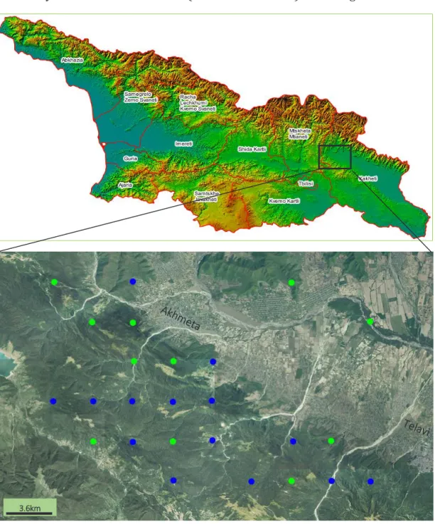
2.1. Study sites

The study sites are near Akhmeta (42° 03'N, 45° 21'E) in the region of Kakheti, Georgia.

Figure 1: Map of the study sites around Akhmeta and Telavi, Kakheti. Green the clusters with signs of degradation and blue clusters without degradation.

These sites are part of the permanent grid of the first Georgian National Forest Inventory which is going to take place on a national level in spring 2019. The goal was to test the developed methods for the upcoming inventory and use the data to improve them. The

(14)

field teams consisted of five Georgian experts, two German experts, and me as a trainee. We worked in pairs. The field work took place in the first week of May 2018 but had to be stopped after 22 clusters due to weather changes. The remaining three clusters were completed during a second field trip in the middle of July 2018.

2.2. Sample design

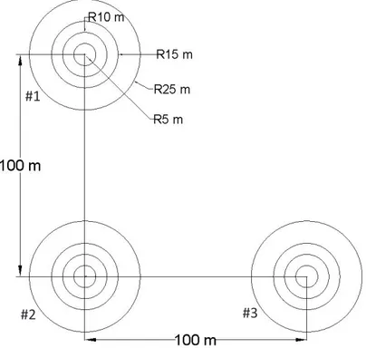
The clusters are part of a grid 3.6 km x 3.6 km spread all over the country and comprises to approximately 1750 cluster that are pre-assessed as forest. Every cluster contains three sample plots. The sample plot centers are located at pre-defined coordinates. The sample plots of each cluster are arranged in the shape of the Latin letter “L”. The center of the sample plot #2 is always the crossing point of the (underlying) grid, and its center defines the location of the entire cluster. The centers of the remaining sample plots are located exactly 100 m North (sample plot #1) and 100 m East (sample plot #3) of this location (Fig. 2).

Figure 2: Schematic structure of the cluster with three sample plots.

A sample plot consists of several concentric circles (Fig. 3) with pre-defined radii (5, 10, 15 and 25 m, respectively). Trees are selected for measuring according to their diameter class and are assessed up to a specific radius (Fig. 3). The elevation as well as exposition are recorded using the sample point center and the overall exposition of the sample plot. The slope angle is measured across the center point and used for the exposition. But there

#1

(15)

is no minimum inclination to determine the exposition. For the analysis the elevation and exposition of sample plot #2 was used since it is defined as the center of the cluster. Where there was no sample plot #2 because of inaccessibility the sample plot #1 or #3 were used depending which one was accessible.

2.3 Variables measured

Most stand information is recorded in the plot of 15 m radius, for example, erosion, forest function, grazing, ground cover, crown closure etc. Most of these variables rely on eye estimation and thus can differ depending on the team that visited the plot. To avoid differences, trainings will be conducted, and control measures are taken to detect teams that do not follow the field manual with thorough description of the indicators and criteria of each categorical variable.

Figure 3: Schematic structure of the nested plot design indicating the different thresholds of DBH for each radius and the regeneration plots.

(16)

The regeneration is measured in two sub-sample plots of 1.5 m radius and in 5 m distance from the sample plot center to the North and to the South as indicated in Figure 3. All species with a diameter at breast height (DBH) less than 8 cm are recorded, in case they are judged to later be part of the upper canopy layer under the current conditions. The regeneration is moreover divided in the three different height classes 1) 0-50 cm; 2) 0.5 m - 1.5 m; 3) >1.5 m. The registration is made species-wise within the height classes. All trees species with diameters greater than the thresholds assigned to the three concentric circles (5, 10, and 15 m) were measured.

The trees recorded, are all living or broken trees. The data gathered includes among other things species, DBH, habitat features as well as different kind of damages (Tab. 1). Damages on the trees are assessed by the field teams through eye estimation.

Table 1: Tree damage categories

Before estimating the damage of the trees, during the evaluation of the sample plot the team already looks for signs of degradation on the 15 m plot level. The judgement of tree damages is independent from the assessment of forest degradation. It is possible that only a small number of trees is recorded “damaged”, although the plot is judged to be degraded. The reason for that is the concentric sample plot design which does not record all trees. However, both, tree damage categories and degradation categories should give indications on how much of the forest is degraded due to anthropogenic activity. There are six forest degradation categories (Tab.2).

Table 2: Forest degradation categories

Stands of low density, number of stems/basal area (artificially opened-up) Timber quality reduction because of exploiting cuts (non-systematic) Damage caused by Phyto- and Ento-pests

Fire affected Grazing

Others (need to be specified)

Damage through logging and/or skidding activities Fire damage

Insect pests / Fungi

Animal damage (e.g. bark peeling) Uprooted-broken tree (natural causes)

Other anthropogenic damage (e.g. pruning for fire wood) Other

(17)

The following figures will give a better picture on what the first two forest degradation categories look like.

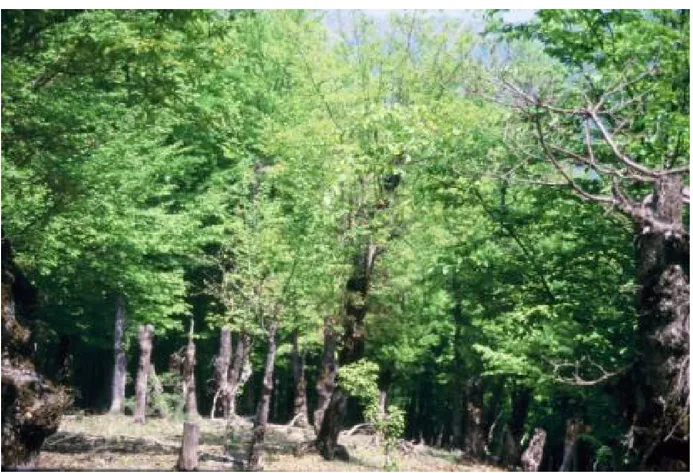
Stands of low density area categorized by a lower number of stems and an incomplete canopy cover but no reduced timber quality in the remaining stand (Fig.4).

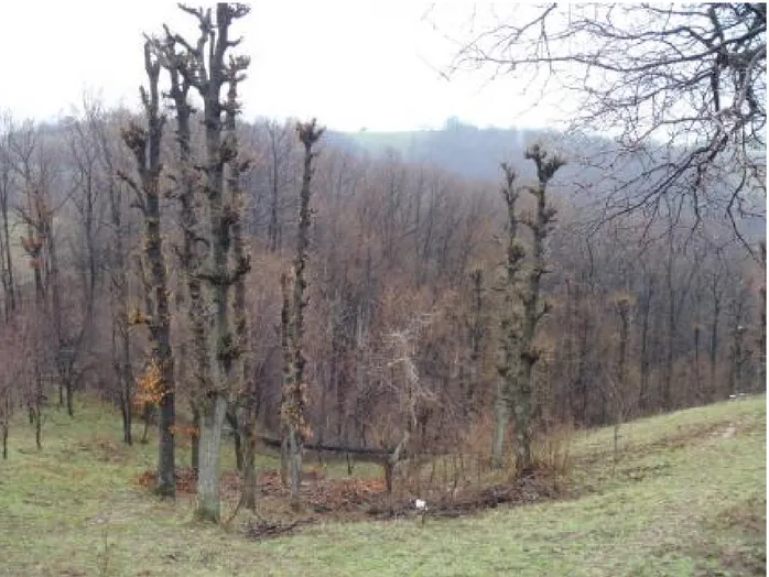
Extreme exploiting cuts look like Figure 5, where timber quality reduction is immediately visible, and the canopy cover is only partially present. Even if this affects only a small area of the plot it is reflected in the protocol as degraded.

(18)

Figure 5: Timber quality reduction because of exploiting cuts

The clusters were divided into two groups; with signs of degradation and without. The plots without will be referred to as non-degraded because parts of these plots cannot be defined as natural forest since it is strongly influenced by anthropogenic activity without being degraded.

Table 3: Number of clusters and sample plots per data set

Non-degraded Degraded

Number of clusters 14 11

Number of sample plots 36 32

The difference in number of sample plots is lower than expected looking at the number of clusters. The reason for that is that some clusters of the non-degraded forest were categorized as non-forest, or non-forest land due to different reasons like the center of the sample plot was in a river bed or on an open area bigger than 0.5 ha. The teams decide in the field that those sample plots should be recorded as no forest because they are not forest according to the definition used in Georgia.

(19)

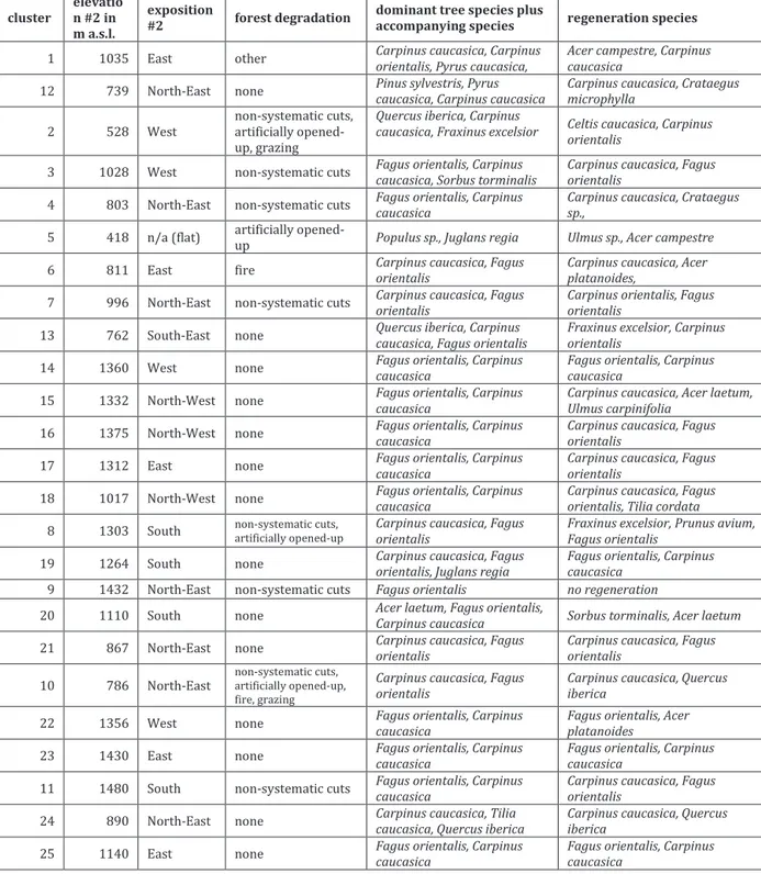
Table 4 gives an overview of the clusters, their degradation, exposition, elevation, the dominant tree species and regeneration.

Table 4: Overview of the clusters recorded

cluster elevation #2 in m a.s.l.

exposition

#2 forest degradation dominant tree species plus accompanying species regeneration species

1 1035 East other Carpinus caucasica, Carpinus _{orientalis, Pyrus caucasica,} Acer campestre, Carpinus _caucasica 12 739 North-East none Pinus sylvestris, Pyrus _{caucasica, Carpinus caucasica} Carpinus caucasica, Crataegus _microphylla

2 528 West non-systematic cuts, artificially opened-up, grazing

Quercus iberica, Carpinus

caucasica, Fraxinus excelsior Celtis caucasica, Carpinus _orientalis

3 1028 West non-systematic cuts Fagus orientalis, Carpinus _{caucasica, Sorbus torminalis} Carpinus caucasica, Fagus _orientalis 4 803 North-East non-systematic cuts Fagus orientalis, Carpinus _caucasica Carpinus caucasica, Crataegus _sp., 5 418 n/a (flat) artificially opened-_up Populus sp., Juglans regia Ulmus sp., Acer campestre

6 811 East fire Carpinus caucasica, Fagus _orientalis Carpinus caucasica, Acer _platanoides, 7 996 North-East non-systematic cuts Carpinus caucasica, Fagus _orientalis Carpinus orientalis, Fagus _orientalis 13 762 South-East none Quercus iberica, Carpinus _{caucasica, Fagus orientalis} Fraxinus excelsior, Carpinus _orientalis 14 1360 West none Fagus orientalis, Carpinus _caucasica Fagus orientalis, Carpinus _caucasica 15 1332 North-West none Fagus orientalis, Carpinus _caucasica Carpinus caucasica, Acer laetum, _{Ulmus carpinifolia} 16 1375 North-West none Fagus orientalis, Carpinus _caucasica Carpinus caucasica, Fagus _orientalis 17 1312 East none Fagus orientalis, Carpinus _caucasica Carpinus caucasica, Fagus _orientalis 18 1017 North-West none Fagus orientalis, Carpinus _caucasica Carpinus caucasica, Fagus _{orientalis, Tilia cordata}

8 1303 South non-systematic cuts, _{artificially opened-up} Carpinus caucasica, Fagus _orientalis Fraxinus excelsior, Prunus avium, _{Fagus orientalis} 19 1264 South none Carpinus caucasica, Fagus _{orientalis, Juglans regia} Fagus orientalis, Carpinus _caucasica

9 1432 North-East non-systematic cuts Fagus orientalis no regeneration

20 1110 South none Acer laetum, Fagus orientalis, _{Carpinus caucasica} Sorbus torminalis, Acer laetum

21 867 North-East none Carpinus caucasica, Fagus _orientalis Carpinus caucasica, Fagus _orientalis 10 786 North-East non-systematic cuts, artificially opened-up,

fire, grazing

Carpinus caucasica, Fagus

orientalis Carpinus caucasica, Quercus iberica

22 1356 West none Fagus orientalis, Carpinus _caucasica Fagus orientalis, Acer _platanoides 23 1430 East none Fagus orientalis, Carpinus _caucasica Fagus orientalis, Carpinus _caucasica 11 1480 South non-systematic cuts Fagus orientalis, Carpinus _caucasica Carpinus caucasica, Fagus _orientalis 24 890 North-East none Carpinus caucasica, Tilia _{caucasica, Quercus iberica} Carpinus caucasica, Quercus _iberica 25 1140 East none Fagus orientalis, Carpinus _caucasica Fagus orientalis, Carpinus _caucasica

(20)

Down deadwood is estimated and measured in the 5 and 10 m plots. Deadwood is defined as broken trees that either fell due to natural causes or were cut and left in the forest.The down dead-wood diameter is measured on its thick and on its narrow end. Down dead wood ≥ 10 cm at the thicker end is recorded in the 5 m radius sub plot. Down dead wood ≥ 20 cm at the thicker end is recorded in 10 m radius sub plot. In case the major part of the down deadwood is inside the sub plot, but the thicker end is outside of the respective sub plot, this down deadwood is not recorded. There are three decay categories that are recorded additional to the length and diameter (Tab. 5).

Table 5: Decay classes of down deadwood Decay class Description

1 Fresh - bark is on and wood is hard

2 Medium decayed - bark partly is off, wood is soft 3 Heavily decayed - bark is completely off, wood is rotten

To record the data a modified and adjusted survey of the Open Foris software developed by Food and Agriculture Organization (FAO) was used. FAO developed this tool to support National Forest Inventories globally. It consists of several components. In Open Foris Collect data are gathered and then transferred into a more user-friendly interface, Collect Mobile. After the fieldwork the data was imported into the Collect database and the relevant data was exported into csv-files for cleansing. The cleansing and preparation of the data was mainly done in Excel. Validation and plausibility checks take place already in the Open Foris Collect Mobile when entering the data, or at the latest when importing it to Collect database.

2.4 Analysis

For the analysis the data sets are divided into two groups. One group showing signs of forest degradation and the other without any disturbance. In the analysis the two data sets are compared to look for differences in basal area, regeneration, number of trees, DBH classes distribution, deadwood, and biodiversity. Because of the sampling design each tree is part of one of the three nested plots according to its DBH since the circles represent different thresholds. Thus, the expansion factor is different due to this design. The small sample size makes it impossible to model a height diameter curve since only a small part of the measured trees is measured for height and not all species are represented. Biodiversity is analyzed using the R-package “vegan” which is made for community ecology and has some of the diversity analysis functions already embedded.

(21)

3. Results

3.1 Cluster outline

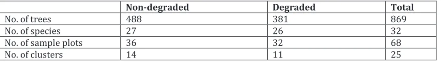
A total of 25 clusters was analyzed including 869 trees, 31 species, and 68 sample plots. The data was divided into two sets representing degraded and non-degraded plots (Table 6). Both sets were well balanced, though the non-degraded had more clusters and sample plots but the difference was rather small. The number of trees of these data sets, however, was greater in the non-degraded plots, where 107 trees more were measured.

Table 6: Statistics on the two data sets

Non-degraded Degraded Total

No. of trees 488 381 869

No. of species 27 26 32

No. of sample plots 36 32 68

No. of clusters 14 11 25

3.2 Exposition and altitude

Exposition as well as altitude were recorded for all sample plots and the values of the #2 sample plot were used as a representative value for each cluster (Fig.6).

Figure 6: Exposition according to number of clusters it occurred in degraded and non-degraded.

0 1 2 3 4 N NE E SE S SW W NW n/a

Exposition of the degraded clusters degraded 0 1 2 3 4 N NE E SE S SW W NW n/a

Exposition of the non-degraded clusters

(22)

The non-degraded stands were mainly exposed towards the North-East, North-West and East, whereas the degraded stands did not face North-West at all. In one degraded cluster the exposition could not be measured because there was no inclination. The altitude of the degraded forests ranged from 418 m a.s.l. to 1480 m a.s.l. and in the non-degraded from 739 m a.s.l. to 1430 m a.s.l. When comparing the two data sets, the degraded plots were mainly found in lower altitudes; 8 out of 11 clusters were found below 1100 m a.s.l.

3.3 Distribution of degradation categories and tree damages

The degradation was recorded per plot. Figure 7 shows that most plots with signs of degradation had either non-systematic cuts (mainly illegal logging activity, timber quality reduction) or were opened-up artificially (incomplete canopy cover). However, there were no plots with degradation due to natural reasons, insect pests or fungi. Each plot can have several forest degradation categories at the same time. Some of the plots had up to three categories while others had none within the same cluster.

Figure 7: Number of plots and type of forest degradation.

Trees with signs of damage were recorded if they were within the concentric circles. Most visible damages on measured trees were in the degraded plots through logging 36% and fire 22%. Among the non-degraded plots, pests made up 55% of all the damaged trees. Looking at the two data sets (Fig. 8), there are 33 trees per ha damaged in the non-degraded and 92 in the non-degraded. This equals 6% in the clusters without degradation and 16% with degradation compared to the total number of trees per ha.

0 2 4 6 8 10 12 Non-systematic cuts Artificially opened-up stands Grazing Fire affected Insect pests or fungi Other

(23)

Figure 8: Dashed the damaged trees per ha of the degraded forest stands and solid the damaged trees per ha of the non-degraded stands.

In the degraded plots mainly Carpinus caucasica was damaged throughout all categories. Whereas in the non-degraded forest pests infected different tree species of which Fagus

orientalis and Carpinus caucasica made up roughly 30% each.

3.4 Tree species in the two categories

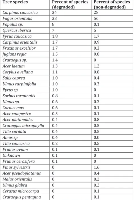
The dominant tree species are listed in the table below (Tab. 7). In total 31 species were identified. In the degraded forest Carpinus caucasica and Fagus orientalis make up two thirds of the observed trees whereas in the non-degraded forest Fagus orientalis dominates with 56%. Other common species of both forests are Quercus iberica, Pyrus

caucasica and Acer laetum.

0 10 20 30 40logging anthropogeni c fire pests unknown

Damaged trees per ha (degraded forests) 0 10 20 30 40logging anthropogenic fire pests unknown

Damaged trees per ha (non-degraded forests)

(24)

Table 7: Percentage of the trees of the degraded and non-degraded forests

Tree species Percent of species

(degraded) Percent of species (non-degraded)

Carpinus caucasica 34 28 Fagus orientalis 33 56 Populus sp. 8 0.1 Quercus iberica 7 5 Pyrus caucasica 1.8 1.7 Carpinus orientalis 1.7 0.9 Fraxinus excelsior 1.7 0.3 Juglans regia 1.5 0.8 Crataegus sp. 1.4 0 Acer laetum 1.3 1.2 Corylus avellana 1.1 0.8 Salix caprea 1.0 0.4 Ulmus carpinifolia 1.0 0.3 Pyrus sp. 1.0 0 Sorbus torminalis 0.8 0.1 Ulmus sp. 0.6 0.3 Cornus mas 0.6 0.1 Acer campestre 0.5 0.1 Acer platanoides 0.4 0.8 Crataegus microphylla 0.4 0.5 Tilia cordata 0.4 0.5 Alnus sp. 0.4 0.0 Tilia caucasica 0.2 0.5 Prunus avium 0.1 0.1 Unknown 0.1 0 Prunus cerasifera 0.1 0 Pinus sylvestris 0 1.6 Acer pseudoplatanus 0 0.4 Malus orientalis 0 0.2 Ulmus glabra 0 0.2 Cerasus microcarpa 0 0.1 Crataegus pentagina 0 0.1

In the degraded forest six clusters are dominated by Carpinus caucasica, three by Fagus

orientalis, one by Populus sp. and one by Quercus iberica. The accompanying species in the Carpinus caucasica stands are mainly Fagus orientalis, Pyrus sp., Crataegus sp., Acer sp. and Quercus iberica. These stands have a total of 18 different accompanying species with a

maximum of nine per cluster. Whereas the Fagus orientalis dominated stands have a total of up to nine different species with a maximum of six.

In the non-degraded data set 8 clusters are dominated by Fagus orientalis, three by

(25)

dominant accompanying species for the Fagus orientalis stands is Carpinus caucasica. But different species of Ulmus, Acer and Tilia along with Corylus avellana and Salix caprea can be observed as well. In the non-degraded forests the number of accompanying species reaches a maximum of 12 in the Fagus stands and 13 in the Carpinus stands. Looking at the species distribution along the altitude gradient (Fig. 9), other species, in particular

Quercus iberica, Populus sp. and Pinus sylvestris occur in lower altitudes whereas Fagus orientalis dominates in the altitudes higher than 1000 m a.s.l. The plots dominated by

species other than Carpinus caucasica or Fagus orientalis show a higher biodiversity in the biodiversity analysis. Their altitude is mostly below 800 m a.s.l. which in turn suggests that they are part of the area where land-use overlaps.

Figure 9: Dominant tree species per cluster according to altitude distribution (Clusters 1-11 are degraded and 12-25 are non-degraded).

3.5 Basal area

The mean basal area per ha in the degraded forests is 19 m² but varies from 9 m² to 30 m². In the non-degraded forests the mean is 21 m² with a minimum of 3 m² and a maximum of 32 m² (Tab. 8, Fig. 10).

(26)

Table 8: Basal area and number of stems per ha in the degraded and non-degraded stands

Degraded forests Non-degraded forests

cluster BA/ha N/ha cluster BA/ha N/ha

1 18 1280 12 11 359 2 20 1072 13 30 482 3 30 637 14 24 282 4 9 242 15 27 253 5 22 111 16 31 514 6 14 398 17 20 515 7 14 809 18 24 323 8 24 778 19 28 945 9 23 261 20 3 509 10 25 251 21 18 274 11 14 189 22 32 463 23 19 647 24 10 1153 25 17 416 Mean 19 553 21 509 SD 6.2 393.2 8.7 258

(27)

3.6 Number of trees and diameters

The mean number of trees per ha are 481 for the non-degraded category ranging from 252 to 1.153 and 553 in the degraded with a minimum of 111 and a maximum of 1.280 (Fig. 11, Tab. 8).

Figure 11: Number of trees per ha per cluster.

Figure 12: Relative distribution of the number of trees per DBH class ( 1: 8-17.9 cm, 2: 18-27.9 cm, 3: 28-37.9 cm, 4: 38-47.9 cm, 5: 48-57.9 cm, 6: 58-67.9 cm, 7: 68-77.9 cm, 8: 78-87.9 cm, 9: 88-97.9 cm, 10: 98-107.9 cm, 11: >108 cm). 69 17 7 4 ₂ 0, 96 0, 08 0, 08 0, 08 0, 08 0, 16 54 24 11 5 ₃ 1, 4 0, 41 0, 41 0, 08 0, 08 0, 08 0 10 20 30 40 50 60 70 1 2 3 4 5 6 7 8 9 10 11 Per cen ta ge per D BH cl as s DBH class

Relative distribution of the DBH classes

(28)

The relative distribution of the number of trees per DBH class and ha was also observed and shows that there are expressed as a percentage fewer trees found in the bigger diameter classes (Fig.12), but most of the trees have diameters between 8 cm and 30 cm.

3.7 Crown closure

Despite the fact, that most of the stands with signs of degradation were described as either artificially opened-up or with non-systematic cuts. The degraded plots have a mean of 64% canopy cover with a minimum of 27% and a maximum of 80%, whereas the non-degraded plots vary between 30% and 86% with a mean of 66%.

Figure 13: Average crown closure percent per cluster in the degraded and non-degraded forests.

3.8 Regeneration

The regeneration was measured for the degraded and non-degraded clusters. On average the degraded clusters had 20.449 and the non-degraded 13.440 seedlings per ha. The degraded forest had one cluster with an extreme high number of seedlings (Fig.14).

(29)

Figure 14: Regeneration, number of seedlings and young trees per ha

Besides the outlier in the degraded forest, the regeneration and basal area are lower in the degraded forest than in the non-degraded forest (Fig. 15).

Figure 15: On the left the relationship between regeneration and basal area; on the right the relationship between regeneration and crown closure.

(30)

3.9 Down deadwood

The degraded stands have a mean of down deadwood of about one third (5 m3_{/ha) of the} volume compared to the total of non-degraded stands (14 m3_{/ha). The difference is} caused by the cluster #25 with 91 m3_{/ha (Fig.16) and the small sample size. Except for} this outlier the volume of deadwood is similar. Without the outlier the average amount of deadwood would be 8 m3_{/ha for the non-degraded plots.}

Figure 16: Down deadwood in m3 of the non-degraded and degraded-forests. 3.10 Overall tree species diversity

The tree species diversity of all tree species was analyzed with the Simpson index for biodiversity (Fig. 17). This index ranges from 0 to 1, where values closer to 1 represent more diverse forests.

(31)

The degraded plots have an average of 0.59 and the non-degraded – of 0.55. When species are evenly distributed it can also contribute to a higher number which in turn gives not only an indication on the diversity but also the evenness of the distribution. In the degraded forests more individuals of the same species occurred whereas in the non-degraded less species, but a greater mixture was found.

(32)

4. Discussion

4.1 National Forest Inventory

This study was part of a pilot study in preparation of the upcoming national inventory in Georgia. Its purpose was to see if the data gathered is sufficient to study and understand the potential of the Georgian forest but also its threats. Including the current condition of the forest and its use, but also how it could be changed in the future. On the one hand having the economic perspective in terms of what timber, of which quality is available in Georgia, on the other hand, having the ecological perspective of nature conservation, biodiversity and sustainability. In addition, it includes to understand the impact of natural and anthropological hazards, like pests, wild fire, or wood pasture. One specific problem in this study was to examine whether the data can be used to reflect upon the differences between degraded and non-degraded forest. For Georgia this is especially important since there is no reliable national data on the condition of the forest; thus, different stakeholders speculate on the loss of forest cover, land-use change and illegal logging (Matcharashvili 2012, Garforth et al. 2016, Global Forest Watch 2019). The National Forest Inventory is consequently crucial for the Ministry of Environmental Protection and Agriculture to support decision making processes and promote a sustainable forest management.

Before going into detail, it should be mentioned that it was rather difficult to find significant differences between the two data sets. The design is made in a way that it should give a good estimate of the whole country once all clusters are taken. The grid is not designed for a small-scale inventory like in this study with an area of roughly 30 000 ha of forest and 25 clusters. The methods of measurements moreover, are designed for a large-scale inventory, many categorical variables are estimates to have an idea of the condition and properties on a stand level. In this study calculations of significance between studied differences were not made, since the statistical requirements for such analysis were not fulfilled and results should therefore be regarded indications. Nevertheless, the results will be discussed in the following paragraphs.

4.2 Altitude and species composition

Species composition and accessibility correlate with altitude. Plots with a higher elevation are in most parts of the study area situated further away from settlements. These plots show less signs of degradation. Easily accessible plots are more likely to be degraded and were found in lower altitudes less than 1100m a.s.l. and closer to the inhabited area. In contrast, plots of the non-degraded forest are located at an altitude of more than 1100m a.s.l., thus they are more difficult to access. The degraded clusters show

(33)

mainly signs of non-systematic logging which results in a lower quality of timber or they were artificially opened-up. Which means they still have higher quality timber within the stands but an incomplete canopy cover. The main reason for these two categories seems to be illegal logging activities (Matcharashvili 2012, Garforth et al. 2016). The accessibility includes not only distance but also the terrain of the area. Most of the Georgian forest is situated on slopes with an angle of more than 30 degrees (Nakhutsrishvili 2013). This inclination also restricts illegal logging to more accessible areas and thus protects the forest in some areas.

Regarding altitude the change in dominant tree species coincides with their natural altitude range. For Fagus orientalis it is between 1000 and 1800 m a.s.l. in this region (Nakhutsrishvili 2013). Since most of the plots have either a beech-hornbeam or a hornbeam-beech forest the main difference between degraded and non-degraded plots depends on the altitude rather than the exposition. Fagus orientalis occurs as dominant tree species starting from 1000 m a.s.l. whereas Carpinus caucasica dominates most of the stands in lower altitudes. The main reason for that could be the different structure of the forest in the lower altitudes. Through the degradation trees of different diameters were removed which creates a structure similar to selection cuttings and in this case it promotes the growth of understory. In the overlapping areas the hornbeam dominated plots are in general lower which allows shrub species like e.g. Crataegus sp. to be part of the upper layer. Moreover, it seems that in the lower altitudes Carpinus caucasica is able to adapt better to the changing circumstances and thus seems to be able to outcompete

Fagus orientalis under these conditions. Also, the amount of precipitation as well as the

soil will affect the abilities of both tree species to their advantage or disadvantage. As a consequence, precipitation and soil should be considered when looking more detailed into the existing species, their spatial distribution, the growing region, and the site conditions.

Quercus iberica, the third most dominant tree species occurring in both data sets is

observed in the lower altitudes with southern exposure. It would be expected to be more present in the degraded forests due to the disturbance and, thus, the possible higher availability of light. However, looking at the crown closure there is almost no difference between degraded and non-degraded plots; consequently, Quercus iberica equally occurs in both degraded and non-degraded forests. Pyrus caucasica is the fourth most common species which could be due to the overlapping of grassland, orchards, and forest. In these overlapping areas mainly Carpinus caucasica, Pyrus caucasica and other woody shrub species like Crataegus sp., Cornus mas, Swida australis or Coryllus avellana build the first and second layer of the canopy. Such forests were described by Nakhutsrishvili (2013) as derivatives of oak forests that transformed into Carpinus caucasica dominated stands with shrub communities. Their structure differs from the forests in higher altitudes in terms of species composition as well as lower tree height.

(34)

4.3 Single tree damages and other damages

The single trees are monitored for signs of damages. Since the degraded plots are mainly degraded due to illegal logging most single tree damages are because of logging activities. These logging damages will, in the future, effect the timber quality which consequently means that, though a forest might no longer seem degraded, it still suffers from the long-term effects on the diameter growth and bole quality (Clatterbuck 2006, Tavankhar et al.2015). Damages from logging affect not only the stand dynamic and the ecosystem as a whole but weaken single trees and make them more susceptible to fungi and insect pests. In the non-degraded plots, the single tree damage is mainly caused by either fungi or insect pests. Since the survey does not differentiate between these two categories, it cannot be determined which of them caused more damages. To know if the trees have fungi or insect related damage another variable that is not analyzed in this study but is part of the NFI inventory protocol could be cross-checked. This means, each tree is checked for habitat features which includes also larger fungi or special insects. If signs of either of those are visible on the stem, it is noted. For a more detailed analysis of the damages a cross-check could thus help to differentiate the pest damages into fungi and insect categories.

4.4 Canopy cover

Crown closure is a variable that is recorded using eye estimation. Due to this approach the estimate can vary greatly which makes interpreting the results difficult. The two data sets show no difference in canopy cover, which gives raise to the question why there is no correlation for some of the degradation categories. The field teams on average estimate the canopy cover relatively high. Which means that the degraded and non-degraded plots do not show any differences regarding canopy cover.

In parallel to the piloting activities a consulting agency elaborated guidelines on the correlation between crown closure and degradation according to their observation in other inventories. These thresholds are mainly relevant for the degradation categories of non-systematic logging activities and artificially opened-up stands. For other degradation categories, a fixed threshold is difficult to determine. Canopy cover thresholds given in the guidelines refer to observations in other countries. Some clusters even being degraded have a higher crown closure than indicated due to big trees with wide crowns or only parts of the plot being degraded. This would suggest that even though there were non-systematic logging activities according to the percentage of crown closure the stand is not degraded. Situations like this should be considered in the training of the field teams and a plan should be established how to proceed in cases like this. The correlation of crown closure and degradation category should be examined more closely to get a

(35)

sharper estimate. To eliminate potential bias the crown closure should be measured more precisely, for instance, using a forest densiometer. Jennings et al. (1999) suggest that eye estimation should be used when dealing with trees that are much taller than the observer. In the present case, a spherical densiometer could help to assess especially plots where not only the dominant layer but also other layers contribute to the crown closure and thus to the light that reaches the ground.

Furthermore, research suggests that crown closure and regeneration are correlated (Madsen&Larsen 1997, Vickers&Palmer 2000, Marchi&Paletto 2010). One would expect that more light would favor regeneration. However, light does not only facilitate regeneration growth but also grass cover which in turn impedes regeneration. Interestingly, two clusters with a crown closure of less than 50% have also a low number of regenerated seedlings which supports the hypothesis that an open canopy does not always facilitate more regeneration. Similar observations were made in Iran where no relationship was found between light intensity and density of the regeneration (Seifidi et al. 2011). Research on the number of seedlings of natural regeneration of the European beech Fagus sylvatica in Slovakia shows that depending on the cutting method applied it varies between 20 000 and 50 000 per ha (Barna&Bosela 2015). There is no comparable study on the natural regeneration of Fagus orientalis, but Vettori et al. (2004) suggest that

Fagus orientalis is genetically speaking ancestral to Fagus sylvatica which consequently

means that similar observations as in Slovakia could be expected in Georgia. In both the degraded and the non-degraded plots natural regeneration barely reaches the minimum of the regeneration measured in Slovakia. Insufficient natural regeneration will have ecological as well as economic implications which are of interest for different parties or stakeholders. Thus, further research should be conducted on this matter with a focus on the differences in regeneration of different degradation categories to rule out assumptions without scientific data as a basis. Due to the similarity in the data sets the current study shows no remarkable difference between the two neither regarding the canopy cover nor the regeneration.

4.5 Basal area

With 21 m²/ha in the non-degraded and 19 m²/ha in the degraded plots the basal area seems low compared to European stands. To give an example, in Slovakia an old-growth natural mixed oak-beech stand located in the Carpathian Mountains on an altitude of 750−1010 m a.s.l. has a basal area of 38 m²/ha (Balanda et al. 2013). Reasons for a lower basal area in Georgia could be the conditions of the site which means having a slope plus a rather low precipitation and dry summers. The non-degraded plots have a lower number of trees per hectare with a slightly higher basal area. It gives the impression that the non-degraded stands have trees of bigger diameter compared to the degraded plots

(36)

where on average more trees are present with a smaller diameter. But the difference in diameter is small with 31.1 cm in the non-degraded and 27.6 cm in the degraded plots and the relative distribution of the DBH classes shows that they are similarly distributed in both plots. The only difference is the number of trees measured and the slight difference in the number of trees per ha. But in general regarding this variable there is also no difference.

The higher number of stems in the degraded plots could be explained by the fact that the bigger trees were taken out artificially which created gaps and gave way to the understory. Examining one of the two dominant tree species of the degraded plots the disturbances caused by the degradation work in favor of Carpinus caucasica (Szwagrzyk et al. 2012).

Fagus orientalis on the other hand is shade tolerant and does not allow much understory

except mainly its own regeneration, in this case having gaps allowed the regeneration to come up quicker and take over these gaps. To produce higher quality timber and improve the stand density further research is necessary to fully understand the reasons that cause the low quality of timber besides the anthropogenically caused degradation. It should not be concluded that all influences on the stand caused by degradation are negative and are the only reason for the condition of the stand. Other reasons could be the overall site condition, including age of the stand, soil as well as water availability. In detail the exposition, position on the slope and the ground cover are factors that need to be considered in the future.

The diameter distributions indicate that selection cuttings have occurred. This implies that most probably trees of different diameters were taken out. However, these cuttings have likely not been made according to the general procedures in a developed selection cutting system. Thus, the stand is closer to an uneven-aged stand than to a high forest. In a managed high forest smaller diameter would be removed sooner to promote the growth of the desired tree species and eventually increase timber quality.

4.6 Biodiversity indices

Clusters 1,2,4,5 in the degraded data set and 12,13,19,20 in the non-degraded show a relatively high biodiversity. Interestingly, each of these clusters has a different dominating tree species. In the degraded it is oak, poplar, beech and hornbeam, while in the non-degraded – oak, pine, maple and hornbeam. These clusters primarily occur on an altitude below 1000 m a.s.l. which leads to the conclusion that they might be part of the communities in the overlapping zones of meadows, orchards and forests. The clusters seem different most probably due to the overlap in land-use. The higher biodiversity index suggests that there might be more species present than in the other clusters.

(37)

A more detailed inventory could be made focusing especially on clusters in overlapping areas to fully understand the potential of these ecosystems. It could be considered to introduce a new variable which indicates land-use overlap. As shown in the diversity analysis the degraded and non-degraded plots with the highest diversity were found in overlapping areas. This moreover demonstrates that land-use overlap does not necessarily mean that the forest is degraded. But should be understood as a forest that might have a different structure or is used differently through e.g. wood pasture.

4.7 Method review

The method used in the pilot study of the national forest inventory is sufficient to respond to general questions about the current state of the forest and give a rough estimate of the standing stock and the tree species composition. To answer more detailed questions about, for instance, the degree of degradation, there are several aspects that need to be considered carefully. The variables chosen to compare the stands were reasonable because according to the definition of the most common degradation categories the degraded plots should be of lower density. The comparison, however, shows that though perceived as stands of low density there was in fact no significant difference between number of trees per hectare, basal area, or canopy cover. This in turn brings up the question why they were indicated as degraded by the field teams. One of the most difficult parts to analyze were subjectively inventoried categorical variables which without proper training and detailed guidelines can be biased depending on the interest, background, or focus of the observer. To minimize this subjectivity careful definitions are essential as well as the will of the observer to actively adjust the personal old view to a new general opinion. Before the piloting activities detailed guidelines were not yet elaborated which might have contributed to an inconsistency in the data and resulted in a relatively poor quality of data for this study. Some of the variables could and should be checked with remote sensing data of the area to improve their quality and to validate them like e.g. elevation or exposition. Using remote sensing would reduce the time spent in the field by having a stronger focus on the stand properties that cannot be determined from the office. Thus, it should be considered for the upcoming inventory to outsource variables that can be determined through other means.

Another factor that should be considered is the effect of logging activities outside the plot since this could affect the canopy cover as well as the growth of the trees inside. Moreover, it might even influence the perception of the observer since after a management activities outside the concentric circles the area might appear more open than it is. The only indicator for logging activity on the sample plot are stumps which are measured as part of the protocol. But those can be also overlooked easily when already partially decayed

(38)

and with a high ground cover. Further research could elaborate on the correlation of the canopy cover dynamic located above different stages of decayed stumps.

To estimate how much of the forest is degraded the sample size needs to be increased, and if done properly and according to the guidelines there should be a clearer distinction between degraded and non-degraded plots. Moreover, the spatial distribution of the different degradation categories could be mapped and possible ways to detect other areas that might be at risk to be degraded should be examined.

After evaluating the plots and comparing the two datasets the author would not take degradation as an independent variable which indicates that this plot is degraded and base the result on this one variable. But the variable should be considered only in combination with other indicating variables which will provide information about the condition of the stand. For instance, cross-checking with erosion, ground cover type, stumps, canopy cover and elevation would already improve the reliability of the indication made. In the future these interactions should be considered, thresholds of the connected variables should be elaborated, and the combined data should be evaluated to fully understand if a stand is degraded and to what extent.

(39)

5. Conclusion

The measured variables provide complex and integrated information on the available timber as well as ecological characteristics of the forest. The analysis of some variables in the degraded and non-degraded plots show that differences are not immediately visible in the data which is most probably because of the small sample size as well as the inconsistent data. Moreover, it was found that degradation appears to be a complex construct and interactions of different variables should be considered. Thus, whether a plot is degraded or not should not be decided based on the observation of the field teams, but it should be seen as an indication that this plot is potentially degraded. To confirm this advice other variables should be considered to decide upon the degradation status of the plot. Considering other variables can help to draw a more precise picture of the stand and, consequently, the subjectivity of the observer will be minimized as much as possible. In addition to the interaction of different variables, the potential of overlapping areas in terms of structure, biodiversity, and land-use should be evaluated separately in the future. The results of this study should be understood as indications of the circumstances under which degradation occurs and the causes of degradation in the area. The methodology seems sufficient for the basic information about the general condition of the stand, but for the upcoming field work the degradation categories need to be better pre-defined, the field teams need proper training to decrease potential bias, and the interaction of different variables need to be considered before deciding whether a stand is natural forest or degraded.

(40)

References

Balanda M., Saniga M., Pittner J., 2013. The development of tree species composition of the species-rich natural forest during the last 33 years. Beskydy 6 (1): 9–16.

Barna M., and Bosela M., 2015. Tree species diversity change in natural regeneration of a beech forest under different management. Forest Ecology and Management 342:93-102.

Bussmann R. W., Paniagua Zambrana N. Y., Sikharulidze S., Kikvidze Z., Kikodze D., Tchelidze D., Khutsishvili M., Batsatsashvili K., Hart R. E. 2016. A comparative ethnobotany of Khevsureti, Samtskhe-Javakheti, Tusheti, Svaneti, and Racha-Lechkhumi, Republic of Georgia (Sakartvelo), Caucasus. Journal of Ethnobiology and Ethnomedicine 12: 43.

Clatterbuck W.K., 2006. Logging damage to residual trees following commercial harvesting to different overstory retention levels in a mature hardwood stand in Tennessee in Proceedings of the 13th biennial southern silvicultural research conference (ed. Connor K.F.) Gen. Tech. Rep. SRS–92. Asheville, NC: U.S. Department of Agriculture, Forest Service, Southern Research Station.

Country monitoring report on Georgia, 2008. Independent monitoring of the implementation of the Expanded Work Programme on forest biodiversity of the Convention on Biological Diversity (CBD POW), 2002-2007. Vasil Gulisahvili Forest Institute, Tbilisi, Georgia.

FAO, 2014. Country report Georgia. FAO Rome.

FAO, 2016. State of the World’s Forests. Forests and agriculture: land-use challenges and opportunities. Rome.

Fehrmann L., Kleinn C., Fuchs H., 2017. Establishing the Georgian National Forest Monitoring System Inventory Protocol. Report for Integrated Biodiversity Management South Caucasus, GIZ. Garforth M., Nilsson S., Torchinava P., 2016. Wood Market Study. Report for Integrated

Biodiversity Management in the South Caucasus, GIZ.

Global Forest Resources Assessment, 2014. Country report Georgia, FAO Rome.

Global Forest Watch, 2019. Tree Cover in Georgia. Global Forest Watch, accessed on 14.03.2019 from www.globalforestwatch.org

Jennings, S.B., Brown, N.D., Sheil, D. 1999. Assessing forest canopies and understory illumination: canopy closure, canopy cover and other measures. Forestry: 72(1).

Kapanadze D., 2014. Georgia: Country Environmental Analysis -- Institutional, Economic and Poverty Aspects of Georgia’s Road to Environmental Sustainability. The International Bank for Reconstruction and Development/The World Bank.

Kochlamazashvili I., Sorg L., Gonashvili B., Chanturia N., Mamardashvili F., 2014. Value Chain Analysis of the Georgian Sheep Sector. Report for Heifer International Project.

(41)

Madsen P. and Larsen J. B., 1997. Natural regeneration of beech (Fagus sylvatica L.) with respect to canopy density, soil moisture and soil carbon content. Forest Ecology and Management 97:95-105.

Marchi A. and Paletto A., 2010. Relationship between forest canopy and natural regeneration in the subalpine spruce-larch forest (north-east Italy). Folia Forestalia Polonica, series A,

Vol.52(1),3-12.

Matcharashvili, I., 2012. Problems and Challenges of Forest Governance in Georgia. Tbilisi, Association Green Alternative, 38.

Mies, E., (2018, October 4). Personal interview.

Nakhutsrishvili, G., 2013. The Vegetation of Georgia (South Caucasus). Springer, Berlin. Parhizkar, P., Sagheb-Talebi Kh., Mataji A., Namiranian, M., 2011. Influence of gap size and development stages on the silvicultural characteristics of oriental beech (Fagus orientalis Lipsky) regeneration. Caspian Journal of Environmental Sciences 9 (1):55-65.

Patarkalashvili T., 2017. Forest biodiversity of Georgia and endangered plant species. Annals of Agrarian Science 15:349-351.

Sefidi K., Marvie M., Mohammad R., Mosandl R., Copenheaver C. A., 2011. Canopy gaps and regeneration in old-growth Oriental beech (Fagus orientalis Lipsky) stands, northern Iran. Forest Ecology and Management 262:1094-1099.

Szwagrzyk J., Szewczyk J., Maciejewski Z., 2012. Shade-tolerant tree species from temperate forests differ in their competitive abilities: A case study from Roztocze, south-eastern Poland. Forest Ecology and Management 282:28-35.

Tavankar F., Bonyad A., Marchi E., Venanzi R., Picchio R., 2015. Effect of logging wounds on diameter growth of beech (Fagus orientalis Lipsky) trees following selection cutting in Caspian forests of Iran. New Zealand Journal of Forestry Science 45:19.

UNDP Georgia (Editor), 2014. Climate Change and Agriculture in Kakheti, UNDP Georgia .

Vettori C., Paffetti D., Paule L., Giannini R., 2004. Identification of the Fagus sylvatica L. and Fagus orientalis lipsky species and intraspecific variability. Forest Genetics 10(3-4):223-230.

Vickers, A.D. and Palmer S.C.F., 2000. The influence of canopy cover and other factors upon the regeneration of Scots pine and its associated ground flora within Glen Tanar National Nature Reserve. Institute of Chartered Foresters, Forestry 73(1).

Zazanashvili, N. and Mallon D., (Editors) 2009. Status and Protection of Globally Threatened Species in the Caucasus. Tbilisi: CEPF, WWF. Contour Ltd., 232 pp.