Reverse Mortgage as an Option for Funding Retirement

Reverse Mortgage as an Option for

Funding Retirement

Master’s thesis within Economics

Author: Sanja Matic

Tutors: Daniel Wiberg Ph.D

Andreas Högberg Ph.D candidate Jönköping May, 2010

Master’s Thesis in Economics

Title: Reverse Mortgage as an Option for Funding Retirement

Author: Sanja Matic

Tutors: Daniel Wiberg Ph.D

Andreas Högberg Ph.D candidate

Date: 2009-05-27

Keywords: Reverse Mortgage, Age Distribution, Home ownership Rates

Abstract

Elderly looking for a way to increase their monthly cash flow or remove mortgage payments, can utilize a reverse mortgage to achieve financial independence and increase cash flow for life. A large number of seniors cannot get traditional “For-ward” loans because they do not have the income to support them, and the reverse mortgage technique is in most cases the only way in which they can get money to supplement their income. In other words, reverse mortgages provide an option for funding retirement. In order to test for a relationship between home ownership rates as dependent variable and explanatory variables I estimate an empirical model by ordinary least squares estimations. The regression analysis is based on average data over the time period 2005-2009. The results of empirical investiga-tion show significant positive effects of GDP and legal origin in all three models. The empirical analysis also confirms the negative relationship between market ca-pitalization and home ownership rates.

Table of Contents

1

Introduction ... 3

2

Theoretical Framework ... 4

2.1 Historical Development of the Reverse Mortgage Market ... 4

2.2 Reverse Mortgage as a Retirement Financing Instrument ... 5

2.3 Available Categories of Reverse Mortgages ... 6

2.4 Advantages vs. Disadvantages of Reverse Mortgages ... 8

2.5 Risks in Reverse Mortgage ... 10

2.6 Guarantees in Reverse Mortgage ... 11

2.7 Moral Hazards in the Reverse Mortgage Market ... 11

3

Previous Research on the Reverse Mortgage Market ... 13

4

Empirical Methodology ... 16

5

Data and Variables ... 17

5.1 Age Distribution ... 17

5.2 GDP percentage change ... 18

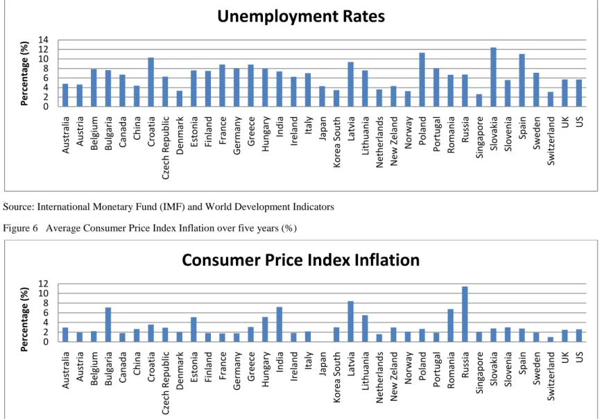
5.3 Unemployment Rates ... 18

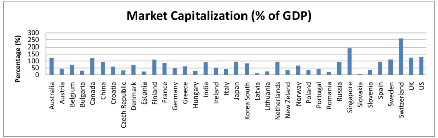
5.4 Consumer Price Index Inflation ... 19

5.5 Market Capitalization as a percentage of GDP ... 19

5.6 House Price Changes ... 20

5.7 Long-term Interest Rates ... 21

5.8 Tax Rates ... 21

5.9 Legal Origin ... 22

5.10 Summary of Explanatory Variables ... 22

6

Descriptive Statistics ... 25

7

Empirical Analysis ... 28

8

Conclusions ... 31

List of Abbreviations ... 33

List of References ... 34

Figures

Figure 1 Annual number of U.S. Reverse Mortgage loans ... 38

Figure 2 Annual number of Australia, Canada, New Zealand, the United Kingdom and United States Reverse ... 38

Figure 3 Average Age Distribution for population age 65 years old and more over five years(%)... 39

Figure 4 Average GDP percentage change over five years (%) ... 39

Figure 5 Average Unemployment Rates over five years (%)... 40

Figure 6 Average Consumer Price Index Inflation over five years (%) ... 40

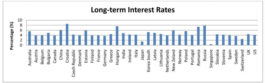
Figure 7 Average Market Capitalization as percentage of GDP over four years (%) ... 41

Figure 8 Average House Price Change over time period (%)... 41

Figure 9 Average Long-term Interest Rates over time period (%) ... 42

Figure 10 Home Ownership Rates (%) ... 42

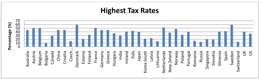
Figure 11 Highest Tax Rates (%) ... 43

Tables

Table 2 Summary of statistics describing the Home ownership Rates (HOR) and the explanatory variables for existing countries, potential countries and both groups (Average over time period 2005-2009). ... 25

Table 3 Pooled-OLS-estimations: Model (1); Model (2); Model (3) ... 28

Appendix

Appendix B ... 39

1

Introduction

The main characteristics of today`s global demographic movements are the problems of population ageing and social uncertainty of seniors due to regular income shortage. Of special concern are individuals with low monthly income, such as retirees, social care system participants, older agricultural population, but especially the older population without regular income in general. Persons aged 60 and more are subject to financial exclusion due to low and unsettled income and old age, therefore they cannot fulfill ri-gid lending conditions of the financial institutions. For this population category, which does not have enough money for covering everyday life expenses but often owns and lives in valuable homes, flats or other real estate`s (“Home rich – Cash poor”) which it does not want to sell, the possibility of supplementing current income through the usage of Reverse Mortgage financing technique has show to be an acceptable and most rea-sonable solution. A reverse mortgage is a financial instrument that allows the elderly homeowner borrowers to access the equity in their home that would otherwise not be liquid, by providing income while not requiring payment as long as the borrower lives in the same house.

This, so far neglected population category from the side of credit institutions, is becom-ing an important target group due to tremendous potential and earnbecom-ing possibilities that reverse mortgage financing offers. At this moment, there is no similar, equally appro-priate and efficient financial model for seniors apart from the reverse mortgage, there-fore, it has an enormous potential for further development and growth not only on the current leading U.S. financial market, but also all over the world. There are numerous opinions concerning the economic potential of the reverse mortgage financing model, but demographic indicators and other prerequisites for a successful expansion show a positive influence on the financial security, healthcare and social care for seniors. The purpose of this thesis is to investigate which variables affect the reverse mortgage market using home ownership rates as proxy dependent variables in the linear regres-sion model. The thesis will also discuss potential problems and risks connected with re-verse mortgage financing and try to point out advantages of usage an expansion of the reverse mortgage financing technique for older homeowners as borrowers, for financial institutions as creditors, but also for the entire society. The data used for analysis is col-lected from a set of 37 countries of existing and potential reverse mortgage markets. The thesis is organized as follows: Section 2 is constructed as a Theoretical Framework, where reverse mortgage is defined and discussed from its historical development, end-ing with advantages vs. disadvantages as well as the risks and guarantees in a reverse mortgage. Section 3 provides a brief review of the literature on previous research re-garding reverse mortgage. The method used in the analysis is explained in Section 4. The data used for empirical analysis and brief explanation of all explanatory variables used in the method is explained in Section 5. Section 6 provides a summary of descrip-tive statistics and explanations of specific results. Also provide Pearson correlation ma-trix table for the explanatory variables to address multicollinearity issues. Section 7 presents the results from the linear regression analysis. Conclusions from the study and suggestions for further research are drawn in Section 8.

2

Theoretical Framework

The ageing population is significant on both a national and international level. It is spe-cifically in developed countries that population ageing and the necessity of assuring more budget reverses for financing retirement, healthcare and other expenses for seniors is becoming a serious problem.

“American has one of the-if not the-most expensive healthcare systems in the world. U.S. spending on healthcare is about two times as much per person as in the whole of the OECD an average, but despite this, life expectancy is not higher than elsewhere.”

(UBS Investment Bank, 2006).

Due to this reason, a growth of interest in reverse mortgage financing can be expected. The rapid growth of the elderly population is of great importance and interest to go-vernmental and financial institutions. Financial institutions need to be more understand-ing regardunderstand-ing demographic trends of the elderly and their demand for credit and finan-cial services including reverse mortgages.

2.1

Historical Development of the Reverse Mortgage Market

Reverse mortgage financing first appeared in Great Britain in the early 1930s (Huan & Mahoney, 2002) in a form of home-equity reversion. They have been available in the United States since the 1960s (Law Reform Commission of Saskatchewan, 2006). Dur-ing the 1970s, the reverse mortgage model appeared in other parts of Europe as well as in Australia, New Zealand and Canada in the 1980s (Ward, 2004; Law Reform Commission of Saskatchewan, 2006). Reverse mortgages, also called Home Equity Conversion or Reverse Annuity Mortgages (RAM), were officially introduced in the U.S. by the Department of Housing and Urban Development (HUD) in 1987, providing greater financial security for elderly American homeowners ages 62 and older (Pratte, 1990).

The most important and long-lived reverse mortgage on the U.S. market is the Home Equity Conversion Mortgage (HECM) offered by the Department of Housing and Ur-ban Development (HUD) in 1987 to accomplish three main objectives: (1) to permit the conversion of home equity into liquid assets to meet the special needs of elderly home-owners; (2) to encourage and to increase the participation of the primary and secondary mortgage markets in converting home equity into liquid assets; and (3) to determine the extent of demand for home equity conversion and the types of home equity conversion mortgages that best serve the needs of elderly households (Szymanoski & E., 1994). This year Congress authorized the HUD to institute a pilot program and issue 2,500 re-verse mortgages. Authorization was increased to 25,000 in the early 1990`s and contin-ued to grow up to this day. HECM program is only insured by the U.S. Federal govern-ment. Research shows that the reverse mortgage market grew slowly during 1990`s. The real boom was reached during last decade, where the number of reverse mortgages in United States continued to double1 each year as older households found themselves in the predicament of being “House rich – Cash poor” (Hendricks, 2003; Max, 2004), but with slow growth rate through the global financial crisis from 2007-2010.

1

According to U.S. Department of Housing and Urban Development (HUD) data, the annual number of reverse mortgage loans in the year 1990 was 157 loans, in 2000 it was 6 640. The number of U.S. re-verse mortgage loans by fiscal year is given in Appendix A, Figure 1.

With the ageing population in the U.S. and the rapid appreciation of residual property, the reverse mortgage industry is designed to prosper. Although reverse mortgages have been part of the mortgage institutions for a long time, their popularity in the U.S. in-creased only a few years ago and functions today as a dominant reverse mortgage fi-nancing model exclusively for America besides the United Kingdom, Canada, Australia and New Zealand.2 The rest of the world is expecting its introduction. The term Equity

Withdrawal Mortgage and Lifetime mortgage used in the United Kingdom is the

syn-onym for the American expression Reverse Mortgage.

2.2

Reverse Mortgage as a Retirement Financing Instrument

People of the age 60 and over without any regular income in general, usually cannot ful-fill rigid lending conditions of the financial institutions. This population category, which does not have enough money for covering everyday life expenses and medical bills of-ten owns and lives in a valuable homes, flat or other real estate (“Home rich – cash poor”). Home equity is an important wealth component for the elderly (Schulz, 1992; Schwenk, 1993). Elderly homeowners can use home equity to supplement their retire-ment income to fund consumption, repair their homes, and finance long-term healthcare as they age (Jacobs, 1986). The problem that many elderly homeowners face is how to tap their housing wealth for consumption without selling their house and relocating. The possible and most reasonable solution to this problem lies in a financial instrument called Reverse Mortgage.

A reverse mortgage is a financial instrument that allows the elderly homeowner borrow-ers to access the equity in their home that would otherwise not be liquid, by providing income while not requiring payment as long as the borrower lives in the same house. Potential borrowers should permanently live in the property and must have proved own-ership in order to ensure possibility of mortgage registration. Borrowers do not have to have income for credit repayment because they do not have that obligation for as long as they live, sell the house or leave the house, and they do not lose any other rights gained by then; he/she has a further right to receive pension or other receipts. In the sit-uation when the retiree moves out or dies, the reverse mortgage lender keeps the mini-mum between the house value and the outstanding debt. The amount of money that could be borrowed via a reverse mortgage generally depends on the borrower`s age and the value of the home. A reverse mortgage loan is available to older homeowners be-tween the ages of 62 and over, regardless of their health condition, exclusively approved on the real estate basis.

Unlike traditional “Forward mortgage” loans, in reverse mortgage lending, the lender pays off the borrower, debt increases over time due to adding of accrued interest but the principal and interest are charged from the value of the property when the loan is closed. Traditional mortgage loan is “Falling debt, Rising equity”, monthly payoffs decrease debt but increase borrower`s part in the value of the purchased house/flat. Reverse mortgage is “Rising debt, Falling equity”, due to pay-off plan, borrower`s share in the value of underlying property decreases and his/her debt increases but there is no repay-ment obligation until the borrower dies, sells or leaves the property.

2

According to U.S. Department of Housing and Urban Development (HUD), Deloitte and Reverse Mort-gage Daily data, the annual number of reverse mortMort-gage loans from the 2005 until 2009 for Australia, Canada, New Zealand, the United Kingdom and United States are given in the Appendix A, Figure 2.

The interest rate on reverse mortgage loans should always be below any other current interest rate in the standard mortgage marketplace, usually calculated on basis LIBOR or 10-year U.S. Treasury bills. As in traditional mortgage lending, the property in re-verse mortgage financing is only an insurance instrument (AARP Foundation, 2008). Depending on the cash flow dynamics in reverse mortgage lending, a borrower`s debt increases with every new cash flow. If the property value increases after the reverse mortgage was taken, there is a possibility of taking out a second or third reverse mort-gage on the difference of increased value. It is important to point out that a borrower`s debt can never exceed the value of the property and the total debt must be paid-out from that value, there is no regress right for charge heirs. The loan balance grows each time the borrower accesses funds from his/her line of credit or receives a monthly payment, and the lender is charging borrower interest on the outstanding loan balance as well as a monthly servicing fee. Loan fees can be paid out of the available loan proceeds. There are no minimum income or credit requirements for qualifying for the reverse mortgage, but there are other requirements that borrowers should satisfy. Since the borrower re-mains the owner of the home, he/she must pay real estate taxes and other conventional payments.

After the borrower dies, his/her heirs/estate must pay off the loan, usually by refinanc-ing it into a forward mortgage or with the proceeds from the sale of the home. The bor-rower or his/her heirs/estate then must facilitate the pay back of the loan using either private funds or selling the home.

After the loan is repaid, all leftover proceeds from the sale of the property go to the heirs or the estate. The lender cannot take the home away if the borrower outlives the loan, the borrower does not need to repay the loan as long as he continues to live in the house and keeps the taxes and insurance current. When the borrower sells his home or no longer uses it for primary residence, he/she or his/her estate will repay the cash re-ceived from the reverse mortgage, plus interest and other fees to the lender.

2.3

Available Categories of Reverse Mortgages

There are three categories of reverse mortgages available in the U.S. market: FHA (Federal Housing Administration) – insured reverse mortgages, public sector revrese mortgages, and private sector reverse mortgages (Devaney, Del Vecchio, & Krause, 1990; Scholen K. , 1985). Public sector reverse mortgages, different from the other two categories, offer a very low cost program to eligible low-income elderly homeowners for the purpose of home repairs, improvements, or for property tax deferral. Private sec-tor reverse mortgages are quite similar to the FHA-insured ones but are usually more expensive to the borrower. The borrower receives a smaller income or monthly payment from the privately underwritten reverse mortgages, everything else is the same (Pratte, 1990).

Two private sector products are available in the market. First, a government-sponsored company that buys and sells mortgages, the largest non-banking financial services com-pany in the world Fannie Mae 1995 has offered a reverse mortgage called the Home-Keeper, and second is the Financial Freedom, currently the largest private reverse mort-gage lender and provider in the U.S., guarantees the Cash Account (Ballman, 2004).

Cash from a reverse mortgage can be received as a lump-sum payment, monthly pay-ments over a fixed period of time, monthly paypay-ments over the remaining lifetime of the borrower if the home is used as principal residence, a credit line that allows the owner to decide how much cash to get and when to get it, and some combinations of the above (Kutty, 1996). Money received from a reverse mortgage is tax-free, because it is consi-dered part of a loan, the property is not sold and the money is not treated as income. In almost all available articles, the possibility to receive cash from a reverse mortgage are defined the same as insured reverse mortgages offer their borrowers. FHA-insured reverse mortgages offer three basic options; tenure, term and line of credit, or combination of all these options. The tenure option provides and guarantees monthly loan payments to the elderly borrower as long as he/she remains in the home. Repay-ment is not required until the homeowner dies or moves out of the home. Tenure reverse mortgage is the most popular type of reverse mortgage. Diventi and Herzog (1991) pro-vide a simulation framework to estimate the amount of a level-payment annuity payable for a tenure reverse mortgage. Merrill (1991), Hancock (1998), Venti and Wise (1991, 2001) and Mitchell and Piggott (2003) calculated the tenure reverse mortgage that would provide the homeowners with monthly payments over the borrower`s remaining life after retirement. In these studies, the maximum amount of reverse mortgage loan is calculated and the lump-sum loan is converted to lifetime annuities with monthly pay-ments.

Under the term option, the borrower gets monthly payments from the lender for a fixed period of time, usually no more than ten years, and repays in a lump-sum when the loan matures. This is considered riskier to elderly homeowners because they may lose their homes at the end of the loan contract. Due to instances when the elderly cannot repay the debt at the end of the term, and are forced to move out of their homes, this form of reverse mortgage is not popular among homeowners.

Elderly who do not need a supplement to their income, but need a lump-sum of money at times for paying large health care bills or home repairs, may choose the line of credit option, which is similar to open-end credit in the financial market.

The monthly payment of a reverse mortgage depends on the following variables: bor-rower`s age (life expectancy), sex (gender), marital status, amount of equity in the house (75%-80% available for loan), mortgage interest rate, ratio of the loan amount to the homes` value, organization cost (e.g., 3% of the principal) and projected rate of appreci-ation in the home`s value (Mayer & Simons, 1994). The monthly or lump-sum payment by a reverse mortgage is positively related to the borrower`s age and the value of home equity, but negatively related to his/her life expectancy and market rates.

Money received from reverse mortgages can be used for any purpose, but first the bor-rower must pay off existing mortgage payments with the proceeds from the reverse mortgage. Many seniors are using these funds for specific purposes (Redfoot, Scholen, & Brown, 2007): eliminating or reducing monthly mortgage payments and remaining in their home, making home repairs, covering health care and everyday life expenses, va-cation, paying off credit cards debts, funding grandchildren`s college tuition, improving their current lifestyle or quality of life.

2.4

Advantages vs. Disadvantages of Reverse Mortgages

The use of reverse mortgages is supported by the life cycle hypothesis3 suggesting that elderly desire to finance consumption by liquidating assets including home equity that were acquired in their younger days (Kutty, 1996). Reverse mortgages would be attrac-tive to elderly homeowners if they become less risk averse and more economically ra-tional. They need to understand the great opportunity cost of not utilizing their housing assets (Peyton & Lotito-Badiollo, 1990). Home equity is the major type of wealth of most elderly (Kennickell & Shack-Marquez, 1992). Appropriate use and management of home equity as an income-generating asset could enhance their economic status and al-leviate their heavy reliance on public benefits during retirement (Burns & Widdows, 1990; Hogarth, 1991).

Reverse mortgages have the advantage of receiving monthly payments, remaining in the home, and having insurance that guarantees the homeowner that he would never owe more than the future value of the house (Mayer & Simons, 1994). If a homeowner relo-cates, the sale of the home can be used to pay off the balance of the reverse mortgage. Advantages of the lump-sum payment from a reverse mortgage are: liquidity for finan-cial emergencies, such as medical bills or house repairs, and consolidation of outstand-ing debts (Mayer & Simons, 1994).

Advantages of home equity conversion include (Rose & Ross, 1993)4:

 No repayments as long as the borrower stay in the home. The borrower cannot be forced from the home to repay the loan.

 Income payments are received income tax-free.

 Payments are not counted as earnings for Social Security or Medicaid purposes.

 Payments continue for the lifetime of the homeowner. Total payments in most cases may exceed the market value of the home. They can exceed if, for exam-ple, the borrower lives very long. However, in fact they hardly actually exceed the value.

 HUD-FHA programs require HUD-approved counseling of the borrower before entering into contract. Counselors are required to discuss alternatives to reverse mortgages.

Whether an elderly person will benefit from a reverse mortgage depends on factors such as desire from proximity to family and friends, emotional attachments to the home, and financial factors (Chinloy & Megbolugbe, 1994).

Despite a number of advantages of taking reverse mortgage as an option for funding re-tirement, we can also construct some possible disadvantages of using this kind of loan. Huck (1987) ascertained that older consumers do not generally like buying on credit. Mason and Bearden (1980) found that one-third of older respondents believed that using credit to buy something is a bad practice. Both lenders and elderly homeowners have been conservative in taking reverse mortgages especially in potential growing countries, because they are new financial instruments and the regulatory provisions are

3

About the life cycle hypothesis in detail see; Modigliani, F., & Ando, A. (1960). The “permanent

income” and “life cycle” hypothesis of saving behavior: Comparison and tests, in I. Friend and R. Jones (eds.) Consumption and Saving, II. Philadelphia: University of Philadelphia.

4 _{See Rose, C., & Ross, J. (1993); “The effective use of the reverse mortgage in financial planning.”}

cient. The orthodox life cycle model predicts that elderly will convert their home equity but the evidence indicates they have not, perhaps because the equity is relatively small for most (Skinner, 1991).

At the end of the loan period, the equity remaining in the home will be substantially re-duced, because the homeowner has received it in the form of monthly loan advances and imputed interest and loan charges. Taking out of reverse mortgage usually implies the bequeathing of a smaller inheritance (Golant, 1992). Although one-third of all elder-ly homeowners have liquid wealth below $5,000, and a reverse mortgage in a lump-sum payment or a line of credit could help in an emergency, many elderly people with child-ren want to pass on this asset to their heirs (Mayer & Simons, 1994). Depending on the state of residence, loan advances from a reverse mortgage may affect eligibility for Supplemental Security Income, Medicaid, and other welfare benefits such as food stamps (Golant, 1992).

Reverse mortgages can be an expensive way to generate cash income, especially in pe-riods of high interest rates. In a reverse mortgage, a borrower is borrowing his/her own money (equity), and for his/her privilege, paying out a substantial amount of interest and loan charges. Persons living alone, especially the very old with lower incomes, may benefit the most in percentage gains in income from reverse mortgages. Unfortunately, many in this very group are living in low-valued homes with low appreciation potential because of declining neighborhoods, and financial institutions do not consider them to be potentially attractive for a reverse mortgage (Golant, 1992).5

Reverse mortgage loans are not recommended for older individuals who have an in-vestment or savings income and less attachment to the home. Elderly couples with the lowest incomes could experience a substantial relative increase in their income flow from reverse mortgages. If an elderly person is willing to move, he/she is better off sell-ing the home and investsell-ing the proceeds than obtainsell-ing a reverse mortgage.

The price of a reverse mortgage may include a flat monthly fee for servicing, origina-tion fee, closing costs such as an up-front mortgage insurance premium (e.g., 2% of ad-justed property value), and other fees (Case & Schnare, 1994).6 Issues in pricing are the use of prevailing house price inflation versus zero rate, type of neighborhood, and de-ferred maintenance and depreciation versus appreciation (Chinloy & Megbolugbe, 1994).7

5

See Golant, S. (1992); “Housing America`s elderly,” Newbury Park, Sage Publications.

6 _{See Case, B., & Schnare, A. (1994); “Preliminary evaluation of the HECM reverse mortgage program.”}

Journal of the American Real Estate and Urban Economics Association (AREUEA), 22 (2) , 301-346.

7 _{See Chinloy, P., & Megbolugbe, I. (1994); “Reverse mortgages: Contracting and crossover risk.”}

2.5

Risks in Reverse Mortgage

The individual borrower, after having chosen to acquire a reverse mortgage, faces the risk of a possibly bankrupt lender. For the lender, the risk surrounding the supply of re-verse mortgages are far more complicated. Philips and Gwin (1993)8 identify several types of risk confronting the reverse mortgage lender:

Crossover Risk – The risk that arises due to the loan value exceeding the value of the mortgaged house. Since the interest rate charged from the borrower is usually higher than the house value appreciation rate, the loan value will certainly exceed the house value at some future point in time, called the Crossover point. The lender will expe-rience loss on every outstanding loan beyond the Crossover point. Important Crossover risks in reverse mortgage are:

1. Occupancy Risk – The attractiveness of the reverse mortgage loan is that it

al-lows the borrower to stay in his/her home until he/she dies. The duration of oc-cupancy will be increase due to increased longevity. Ococ-cupancy beyond the av-erage crossover point will cause loss to the lender.

2. Mobility Risk – The events of a contingency to repay a loan other than the death

of the borrower are called mobility events. One reason could be the selling of a house for refinancing or realizing possible profits on the sale due to favorable real estate trends. Another could be due to health or nursing care. Above average mobility may cause prepayment risk and below average mobility may cause oc-cupancy risk.

3. Interest Rate Risk – In the high interest rate regime, the lenders would find it

dif-ficult to achieve asset-liability matching. Reverse mortgage loan assets are liq-uid, they have every negative cash flow and due to high interest rates, the Cros-sover point is reached earlier than the expected time, which means assets lose value. On the other hand, a higher interest rate might force the lender to yield higher payments on guaranteed investments or bonds.

4. Home Appreciation Risk – If homes do not appreciate as much as expected, the

Crossover point occurs sooner than expected. Property appreciation rates vary depending on the location and the type of property. Even if the general apprecia-tion rate is as high as the rate lender predicts, he might still face the property risk.

Longevity Risk – The risk of the borrower living longer than expected. If a borrower remains in his/her home for a long period of time, there is a greater chance that the val-ue of the loan will exceed the valval-ue of the property.

Antiselection – The risk of a house value being overstated by Intermediaries or Bor-rowers.

Moral Hazard – The risk of a borrower`s improper or negligent maintenance of proper-ty and not taking home insurance or not renewing house insurance in time and not pay-ing property tax.

Litigations – Risks of litigations with heirs during loan repayment or in handing over the property to lender.

8 _{See Philips, W., & Gwin, S. (1993); “Reverse mortgages." Transactions Society of Actuaries, Vol.}

2.6

Guarantees in Reverse Mortgage

There are several different types of reverse mortgage contracts, but all have one thing in common: “The lender pays the borrower rather than vice versa” (NRMLA)9. In other words, the investor promises to pay a homeowner some sum of money, which the homeowner then converts into current consumption. In exchange, the investor accumu-lates interest on the loan and earns a stake in the homeowner`s equity. The home loan is repaid only when the borrower leaves the house due to death, permanent move, or sale. The size of the reverse mortgage, or loan, available to the homeowner is a function of the property`s initial value and projected future appreciation, the owner`s initial home equity, interest rates, and the owner`s age and that of his/her spouse. In the United States, income and credit records are not used to determine the loan value, and the bor-rower`s medical condition cannot be used to underwrite the terms of the loan. These re-verse mortgages provide four guarantees for the borrower, each of which implies risk borne by the lender (Philips & Gwin, 1993):

 Residency Guarantee: The homeowner may remain in the property until death, regardless of the loan balance.

 Income Guarantee: The income support continues as long as the homeowner lives in the home.

 Repayment Guarantee: There is no repayment obligation until the homeowner dies or sells the home.

 Nonrecourse Guarantee: The homeowner`s other assets cannot be used to re-pay the loan.

Guarantees presented above show that reverse mortgages are designed to limit the bor-rower`s and the lender`s exposure to financial loss.

2.7

Moral Hazards in the Reverse Mortgage Market

A house is the major assets for most families across the world. Previous analysis of sur-vey data show that in the absence of a change in family structure, most senior citizens are unlikely to move. Case and Schnare (1994), state that the elderly desire to stay in their homes. In fact, homeownership rates remain virtually unchanged after age 55, even those who move are more likely to move into a large house than a smaller one (Venti & Wise, 1989; Merrill S. R., 1984; Feinstein & McFadden, 1989).

The reason why older people do not want to move from their homes is that people have a deep-seated attachment to their house and presumably their neighborhood. Elderly who own their home are protected from potential rapid increases in rents, which they might face if they sold and entered the rental market. One study found that homeowner-ship rates were much higher in rental markets that demonstrated a lot of volatility (Sinai & Souleles, 2005).10 Given the fact that housing costs are such a large portion of the

9 _{National Reverse Mortgage Lenders Association (NRMLA) is the national voice of the reverse}

mort-gage industry, serving as an educational resource, policy advocate and public affairs center for lenders and related professionals. NRMLA was established in 1997 to enhance the professionalism of the re-verse mortgage business.

10_{See Sinai, T., & Souleles, N. S. (2005); “Owner-Occupied Housing as a Hedge Against Rent Risk.”.}

budget of older households, the elderly should be particularly concerned about big changes in this expenditure (Butrica, Goldwyn, & Johnson, 2005).

Another economic reason why seniors may not want to sell their home is that the house is treated favorably under Medicaid and other means-tested benefits programs. Elderly have a lot of reasons why they do not want to sell their homes, but the question is why when they do sell their homes they tend to buy something that costs just as much or even more. The first most important reason is poor health, secondly is their desire to move closer to family, and the third reason for moving is “amenities”, which may in-volve moving to a resort area and higher costs.

With an absence of resources and a borrower`s freedom to determine the date of exit from the home, high concerns of adverse selection and a moral hazard in the reverse mortgage market have been used to rationalize high fees or limited market size (Chinloy & Megbolugbe, 1994; Szymanoski & E., 1994; Caplin, 2002). Adverse selection arises if consumers are expecting an unusually long life, low mobility, or low rates of appreci-ation enter into reverse mortgages at a rate disproportionate to their share of the popula-tion.

Reverse mortgage might have two dimensions of a moral hazard. The first, modeled by (Miceli & Sirmans, 1994) and (Shiller & Weiss, 2000) is that a mortgage or facing de-fault has no incentive to maintain property values. The second moral hazard issue is that by giving funds to an elderly homeowner, life in the home is made relatively more at-tractive than life after moving or death, so the act of giving a borrower a reverse mort-gage may extend the borrower`s stay in the home.

Economists have recognized that reverse mortgage markets may suffer from adverse se-lection and moral hazard problems. Because reverse mortgage loans are not due until a borrower dies, sells the house, or permanently moves out, people who know they are likely to stay in their homes for a long time will find reverse mortgages more attractive than others. Also, economists are concerned that the moral hazard problem on home maintenance would make lenders think twice before entering the reverse mortgage mar-ket. Davidoff (2006)11 showed that homeowners over 75 spend less on routine mainten-ance than younger owners of similar homes. In practice, the moral hazard problem is mitigated because borrowers are the residual claimant of the house, and because lenders are insured against the risk that the proceeds from a home sale fall short of the loan bal-ance.

11_{See Davidoff, T. (2006); “Maintenance and the home equity of the elderly.” UC Berkeley Working}

3

Previous Research on the Reverse Mortgage

Market

Over the years most research on reverse mortgages has focused on their potential mar-ket, technical and financial difficulties in their management. Weinrobe (1987) found that the age of a homeowner and the value of home equity were positively related to the decision to convert home equity. However, the ratio of monthly income to equity, being married, and the homeowner`s child as a principal advisor in the conversion decision were negatively related to home equity conversion.

A series of studies by Venti and Wise (1989, 1990) show that elderly homeowners do not reduce their housing wealth in the absence of precipitating events such as the death of a spouse or entry to a nursing home. If elderly homeowners have strong psychologi-cal attachment to their homes, then reverse mortgages, which generate additional in-come and liquid wealth for elderly homeowners while allowing them to continue living in their homes, may be welfare improving for many households.

Several recent studies have looked more specifically at the potential market for reverse mortgage. Venti and Wise (1991) use the 1984 Survey of Income and Program Partici-pation (SIPP) to estimate the impact of a reverse mortgage on the income and assets of homeowners classified in four age groups: age 55 to 64, 65 to 74, 75 to 84, 85 and over. They found that the median elderly homeowner, even in the lowest third of the income distribution, would only have a small percentage increase in income from a reverse mortgage. Although they note that most elderly could substantially increase their liquid wealth with a lump-sum payment from a reverse mortgage. Venti and Wise conclude that the potential market for reverse mortgages is limited to single persons who are se-niors.

After Venti and Wise`s investigation, Merrill, Finkel and Kutty (1992) used a different data set – the American Housing Survey of 1989 and assumed that the potential market for reverse mortgages is composed of households aged 70 or older, with annual incomes less than $30,000, who have lived in their homes at least ten years, and who own fully paid-off houses valued between $100,000 and $200,000.

A year later, 1993, Venti and Wise concluded that home equity was the only form of wealth that could increase the current income level of the elderly. The majority of households (70%) over age 62 owned their home and most of these (80%) had no mort-gage (Mayer & Simons, 1994). The median housing equity was $64,000 while the me-dian level of liquid assets was $15,000.

Using the same Survey of Income and Program Participation (SIPP) as Venti and Wise but for the year 1990, Mayer and Simons showed that more than six million elderly homeowners have high levels of home equity and could increase their monthly incomes by obtaining reverse mortgages. Although the reverse mortgage payment, as a percen-tage of monthly income, is small for more households, they showed that it would raise income for almost 1.5 million elderly persons above the poverty level. This is due to the fact that most elderly homeowners own their homes free and clear and thus have sub-stantial amounts of untapped home equity. However, since most elderly homeowners have little or no current labor income they cannot qualify for a conventional home equi-ty loan or a line of credit. Mayer and Simons attribute that many elderly households have very little liquid wealth. They suggest that the availability of a lump-sum payment

to protect against various financial shocks that might be related to housing, health care, or automobile care could be very valuable to many elderly homeowners. They use data from the SIPP to illustrate that drawing the full line of credit available in a lump-sum could increase liquid wealth by 200 percent or more for many elderly homeowners. Using a sample of approximately 2,500 loans, Case and Schnare (1994) evaluated HECM borrower characteristics, including the determinants of product choice. They calculated the probability of a borrower choosing each payment option as a function of age, family composition, property value, property location, and other characteristics. Their findings include the following: 1) younger borrowers were more likely to elect te-nure payments; 2) there was not a strong relationship between income and product choice; 3) single men were less likely than women or couples to choose the line of cre-dit option; 4) borrowers with higher valued properties were much less likely to choose the line of credit option; 5) rural borrowers were more likely to choose the line of credit option than suburban or urban borrowers.

The potential size of the reverse mortgage market of 1995 was analyzed by Rasmussen, Megbolugbe and Morgan. They note that there are two motives for obtaining a reverse mortgage: to draw down wealth as one age (life-cycle motive) and to diversify illiquid housing wealth (asset-management motive). They note that for many households the annuity value may not be large, but the addition to liquid wealth is substantial.

Two years later in 1997, Rasmussen, Megbolugbe and Morgan explored the importance of investment motives for obtaining a reverse mortgage and noted how certain expendi-tures, such as long-term care insurance, mid-career human capital investments, and children`s college costs, may be better financed with a reverse mortgage. The ability of a reverse mortgage to make housing equity more readily accessible allows homeowners more flexibility in financing large expenditure. The availability of a line of credit or lump-sum option is necessary for this expanded flexibility. They also note that for some borrowers the term duration, rather than the tenure, fits financial needs better.

In the year 1999, Fratantoni C. Michael sought to explain the determinants of reverse mortgage product choice. A simple theoretical model of the reverse mortgage borrow-er`s product choice is developed using stochastic dynamic programming techniques. Support for the theoretical results is given by multinomial logistic regressions based on a data set of Home Equity Conversion Mortgages. The simulation model shows that if the elderly are primarily concerned with the impact of unavoidable expenditure shocks on their standard of living, they are likely to be better off with a line of credit plan, which gives them access to a large sum of money, rather than adding an additional fixed component to their income.

One year later in 2000, Caplin Andrew has outlined some of the economic forces that may help to explain the gap between the current U.S. market and its theoretical poten-tial. These include transactions costs, moral hazard and consumer uncertainty about fu-ture preferences. In addition he explored some psychological forces that may help ex-plain lack of enthusiasm for these products among the majority of older home owners. He also focused attention on impediments to market development that originate in the legal, regulatory and tax systems.

Davidoff and Welke (2005) have presented a model of reverse mortgage demand that showed selection on the dimension of mobility can be advantageous rather than adverse, because the same characteristics that make spending home equity through a reverse mortgage attractive also make disposing remaining home equity through moving attrac-tive. Empirically, high housing wealth and low non-housing wealth drive both reverse mortgage demand and mobility.

Two years later in 2007, Michelangeli Valentina has used single households from the Health and Retirement Study (HRS) data to study the economic gains or losses asso-ciated with taking out reverse mortgages. These data are examined within a dynamic structural life-cycle model featuring consumption, housing and mobility decisions. These decisions are made in light of lifespan and mobility uncertainty. Model solution and estimation are based on the Mathematical Programming with Equilibrium Con-straints approach. She found that seniors are relatively high risk adverse and home equi-ty is their most important component of precautionary savings. The moving risk togeth-er with the lack of divtogeth-ersification is the main causes of welfare losses for house-rich, but cash-poor. In addition, she concluded that reverse mortgages are a very bad option for house-rich, but cash-poor households.

Bishop and Shan (2008) examined all Home Equity Conversion Mortgage (HECM) loans that were originated between 1989 and 2007 and insured by the Federal Housing Administration (FHA). They showed how characteristics of HECM loans and HECM borrowers have evolved over time. Also they compared borrowers with non-borrowers, and they analyzed loan outcomes using a hazard model. In addition they conducted nu-merical simulations on HECM loans that were originated in 2007 to illustrate how the profitability of the FHA insurance program depends on factors such as termination rates, housing price appreciation, and the payment schedule. Their results also suggest policy makers who are evaluating the current HECM program should practice caution in predicting future profitability.

One year later in 2009, Hui Shan examined HECM loan level reverse mortgage data from 1989 until 2007 and presented a number of findings. He showed that recent verse mortgage borrowers are significantly different from earlier borrowers in many re-spects. Also he found that borrowers who take the line of credit payment plan, single male borrowers and borrowers with higher house values exit their homes sooner than other reverse mortgage borrowers. He also combined the reverse mortgage data with county-level house price data to show that elderly homeowners are more likely to pur-chase reverse mortgages when the local housing market is at its peak. This finding sug-gests that the 2000-2005 housing market booms may be partially responsible for the rapid growth of reverse mortgage markets.

4

Empirical Methodology

The theoretical framework in the previous sections has thoroughly explained important facts in the reverse mortgage market. The United States serves as a market leader in re-verse mortgage financing. In Europe, rere-verse mortgage financing is presented in the United Kingdom, where the Norwich Union is the leading player. Other non-European countries that offer a reverse mortgage financing technique, besides the U.S. are: Cana-da (CHIP is the main provider of reverse mortgages), Australia (The Australian reverse mortgage market now has ten providers) and New Zealand (Sentinel, SAI Life and Life-style Security). Except for the already mentioned “Existing” countries, I have included “Potential” countries, mainly from Europe which have a great potential for introduction and implementation of a reverse mortgage.

This section explains the method used in the analysis to study the relationship between a reverse mortgage market and explanatory variables. Common to most previous studies in the reverse mortgage is that they use some proxy as dependent variable in order to es-timate the empirical model. Unfortunately, data on the total size of reverse mortgage market are only available for the five existing and developed markets. As previous re-searchers, I also used some proxy as a dependent variable. In the linear regression anal-ysis, Home ownership Rates (HOR) is used as dependent variables instead of the total size of the Reverse Mortgage market (RM).

Home ownership rates are one of the main preconditions for a reverse mortgage financ-ing possibility. A potential borrower should permanently live in the property and have proved ownership in order to ensure possibility of mortgage registration. In general, se-nior citizens often own valuable homes more than younger adults, but they often does not have enough money for supplementing current income. Venti and Wise (1993) con-cluded that home equity was the only form of wealth that could increase the current in-come level of the elderly. High home ownership rates give older people material securi-ty and they provide support for a comfortable living standard. The data of home owner-ship rates are not available for each year in the period of investigation for all counties. In the linear regression, variable is used as current percentage rate (Appendix B, Figure 10). To empirically test the relationship between home ownership rates and explanatory variables, I will estimate empirical model by ordinary least squares estimation (OLS). The model for regression analysis is constructed in the following equation:

𝐻𝑂𝑅 = 𝛼 + 𝛽₁ 𝐴𝐷 + 𝛽₂ 𝐺𝐷𝑃 + 𝛽₃ 𝑈𝑅 + 𝛽₄ 𝐶𝑃𝐼_{𝐼𝑛𝑓𝑙𝑎𝑡𝑖𝑜𝑛} + 𝛽₅ 𝑀𝐶𝐴𝑃 +𝛽₆ 𝐻𝑃𝐶 + 𝛽7 𝐿𝑇𝐼𝑅 + 𝛽8 𝑇𝑅𝐻𝑖𝑔𝑕𝑒𝑠𝑡 + 𝛽9 𝐿𝑂

where the intercept parameter of the regression model (constant number) is noted as 𝛼. Betas in the regression represent the slope in the multi-dimensional model, noted as 𝛽. The explanatory variables used in the model are: Age Distribution (AD), GDP

percen-tage change (GDP), Unemployment Rates (UR), Consumer Price Index Inflation (𝐶𝑃𝐼𝐼𝑛𝑓𝑙𝑎𝑡𝑖𝑜𝑛 ), Market Capitalization as a percentage of GDP (MCAP), House Price

Changes (HPC), Long-term Interest Rates (LTIR), Highest Tax Rates 𝑇𝑅_{𝐻𝑖𝑔𝑕𝑒𝑠𝑡} and Legal Origin (LO) which represents the dummy variable.

The definitions of all explanatory variables are explained in the next section where one can also find the summary of variables presented in Table 1.

5

Data and Variables

The data used for the empirical analysis is collected from a set of 37 countries of exist-ing and potential reverse mortgage markets. The time period covered in the regressions is from 2005 until 2009. The data of the explanatory variables in the regression are used as an average over five years (2005-2009).

The 37 countries consist of eight Anglo-Saxon countries represented by Australia, Can-ada, India, Ireland, New Zealand, Singapore, the United Kingdom and United States. The remaining 29 countries have a Civil Law system represented by: Austria, Belgium, Bulgaria, China, Croatia, the Czech Republic, Denmark, Estonia, Finland, France, Ger-many, Greece, Hungary, Italy, Japan, Korea South, Latvia, Lithuania, the Netherlands, Norway, Poland, Portugal, Romania, Russia, Slovakia, Slovenia, Spain, Sweden and Switzerland.

For my analysis I divided countries into three main groups: an “All Reverse Mortgage

Market” of target countries; an “Existing Reverse Mortgage Market” which includes

five countries: Australia, Canada, New Zealand, the United Kingdom and United States, and a “Potential Reverse Mortgage Market” examining the remaining 32 countries.

5.1

Age Distribution

The rapid growth rate of today`s elderly population is becoming a worldwide problem. This neglected population category has been neglected due their age, but from the side of credit institutions is becoming an important target group for the development of a re-verse mortgage. Weinrobe`s (1987) research shows that the age of a homeowner and the value of home equity are positively related to the decision to convert home equity. For my own research, I decided to use an average age distribution variable over five years by country for a population ages 65 years old and over. All available data clearly shows that over the last 25 years the percentage of the worldwide population ages 65 and older all has expanded. If one expects this growth trend to continue, then age distribution will positively affect home ownership rates. Based on data for home ownership rates for all countries, one can conclude that the home ownership rate is higher for elderly, especial-ly for individuals ages 65 and over.

The rapid growth rate of the elderly can increase home ownership rates in the future, which directly represents one of the main predispositions for the development of a re-verse mortgage market. According to Doms and Krainer (2006), demographic change in each demographic group, especially in a group 55 and over, activates an important sti-mulus, which affects the overall homeownership rate. Thus, due to their research one can expect a positive sign in regressions.

According to the World Development Indicators data, in the “Potential” group of coun-tries, Japan (20.98%) has the highest average age distribution over five years for indi-viduals ages 65 and over, whereas India (5%) has the lowest. In the “Existing” group of countries the United Kingdom has the highest average age distribution over five years (15.92%), while New Zealand (12.42%) has the lowest. A graph of the age distribution included in the study is provided in Appendix B, Figure 3.

5.2

GDP percentage change

The Gross Domestic Product (GDP) is a basic measure and an important indicator of the economic situation in each country all over the world. GDP per capita represents the purchasing power of each population and is often positively correlated with the standard of living. By analyzing incomes, Merrill, Finkel and Kutty (1992) assumed that the po-tential market for reverse mortgages is composed of households aged 70 or older, with annual incomes less than $30,000. Also, Mayer and Simons (1994) showed that more than six million elderly homeowners have might levels of home equity and could in-crease their monthly incomes by obtaining reverse mortgages. Although the reverse mortgage payment, as a percentage of monthly income, is low for more households members, they showed that it would raise income for almost 1.5 million elderly persons above the poverty level.

In the situation of small GDP per Capita, elderly people with a home of their own can be stimulated to utilize their home ownership in a way to take a reverse mortgage for supplementing their current income. Based on previous research, the relationship be-tween home ownership and GDP is presented in the model. The data of the explanatory variable in the regression is used as an average percentage change over five years (2005-2009). In the regression one can expect a positive sign between variables home ownership and GDP.

According to the International Monetary Fund (IMF) data, China (10.66%) has the highest average GDP percentage change over five years in the “Potential” group of countries and Italy (-0.44%) has the lowest. Australia (2.84%) has the highest average GDP percentage change over five years in the “Existing” group of countries and the United Kingdom (0.64%) has the lowest. A graph of GDP percentage change included in the study is provided in Appendix B, Figure 4.

5.3

Unemployment Rates

The global economic and financial crisis had led to a dramatic increase in the number of people facing unemployment. Around the world, families are trying to cope with sub-stantial losses of income. Workers everywhere are taking a hit, not just in their jobs, al-so in their homes, as redundant workers across diverse al-social classes realize that they cannot keep up with mortgage repayments or rent.

Oswald (1996) and (1997) provides an impressive array of data indicating a strong posi-tive relationship between home ownership and unemployment. His argument is that homeowners are less willing than private renters to move to jobs when they become un-employed because owners have larger costs of moving than do renters. Based on Os-wald`s research, I have included this explanatory variable in the regression model as an average over five years by country, expecting a positive sign.

According to the International Monetary Fund (IMF) and World Development Indica-tors data, the country with the highest average unemployment rate over five years in the “Potential” group of countries is Slovakia (12.42%) and with the lowest is Singapore (2.63%). The country with the highest average unemployment rate in the “Existing” group of county is Canada (6.70%) and with the lowest is New Zealand (4.34%). A graph of unemployment rates is provided in Appendix B, Figure 5.

5.4

Consumer Price Index Inflation

The global financial crisis of 2007 has resulted in the collapse of large financial institu-tions. The crisis has affected the rapid global rise in inflation in the year 2008. Inflation has resulted in the reduction of wages and savings. With high inflation and difficulties to save up money, the elderly are most affected through daily struggles with a high cost of living. It is because of expensive living costs that senior citizens are forced to find an additional source of financial income.

After World War II, the United States underwent a dramatic rise in home ownership, and by the early 1950s more than half of all U.S. households owned a home. As a result the Bureau of Labor Statistics (BLS) decided to broaden its definition of housing to in-clude items tied to home ownership. Starting in 1953, a separate housing-cost index based on the asset-price approach, which included the price of the asset and the cost of money used to purchase the asset, was introduced into the Consumer Price Index (CPI)12. Owner-occupier housing costs represent the largest single component of the CPI.13 Using average CPI inflation percentage change over five years (2005-2009) in the regression I will estimate its effect on the home ownership. Research suggest that an increase in the CPI raises housing costs, which is why one can expect a positive sign in the regression.

According to the International Monetary Fund (IMF) data, the country with the highest average CPI inflation percentage change over five years in the “Potential” group of countries is Russia (11.43%) and with the lowest is Japan (0.004%). The country in the “Existing” group of countries with the highest average CPI inflation percentage change is New Zealand (2.97%) and with the lowest is Canada (1.81%). A graph of CPI in-cluded in the study is provided in Appendix B, Figure 6.

5.5

Market Capitalization as a percentage of GDP

Market capitalization to GDP measures the size of a country`s stock market relative to the size of its economy. It is an indicator for how well stock markets are developed (Demirguc-Kunt & Levine, 1995). When market capitalization is growing, it creates an overall better situation in the economy and often motivates people to invest money on the stock market rather than in the house market.

Suppose you had put $100,000 into the U.S. property market back in the first quarter of 1987. According to the S&P/Case-Shiller national home-price index14, you would have nearly tripled your money by the first quarter of 2007, to $299,000. On the other hand, if you had put the same money into the S&P 500, and had continued to re-invest the dividend income in that index, you would have ended up with $772,000 to pay with more than double what you would have made on the house. There are three main con-siderations if we want to compare houses and stocks. The first is depreciation: “Stocks do not wear out and require new roofs; houses do.” The second is liquidity: “Houses are

12 _{Consumer Price Index is an inflationary indicator that measures the change in the cost of a fixed basket}

of products and services, including housing, electricity, food and transportation.

13 _{The treatment of owner-occupied housing in the Consumer Price Index (CPI) has long been a subject of}

confusion and consternation. Thus, a session to explore the issues was organized at the National Associ-ation for Business Economics Annual Meeting in Chicago on September 26, 2005., where Carson J., Johanson D. and Steindel C. presented article:”Housing Costs in the CPI: What Are We Measuring?.”

14 _{The S&P/Case-Shiller Home Price Indices measures the residential housing market, tracking changes}

more expensive to convert into cash than stocks.” The third is volatility: “Housing mar-kets since World War II have been far less volatile than stock marmar-kets.”15

Based on these facts, I expect a negative sign of the coefficient in the regression model. The ex-planatory variable is used as the average Market capitalization as a percentage of GDP over four years (2005-2008), since the data for the year 2009 were not published. According to the World Bank data, the country with the highest average market capita-lization over four years in the “Potential” country group is Switzerland (259.65%) and with the lowest is Slovakia (7.2%). In the “Existing” group, the county with the highest average market capitalization over four years is the United States (128.48%) and with the lowest is New Zealand (33.73%); see Appendix B, Figure 7.

5.6

House Price Changes

Many economists consider the financial crises from 2007 to 2010 as the worst financial crises since the Great Depression of the 1930s. An unstable economic situation in a country leads to a reduction in house pricing. In many countries, the housing market has suffered during financial crises. Declining housing prices also resulted in homes worth less than the mortgage loan, providing a financial incentive to enter foreclosure.16 Growth in house pricing can decrease the number of young entrants to home ownership, but houses are becoming more valuable, which means that elderly borrowers of a re-verse mortgage can get higher loan amounts.

With so many homeowners highly leveraged, a small decrease in house pricing can put many homeowners into a situation of negative equity. With no ownership at stake and a large mortgage, some homeowners are more likely to default or sell their house in a surplus market. The excess supply of houses on the market drives down prices further in a downward spiral (Stein, 1995). From this point of view, one can expect a negative sign as a result of the regression model.

“As House prices are increasing, homeownership rates are also increasing!” Low

terest rates and the expected capital gain on the home have made homeownership in-creasingly attractive and inin-creasingly within the reach of those who could otherwise not afford to buy a home, as noted by Federal Reserve Chairman Alan Greenspan (2004). Based on this information, I can also expect a positive sign in the regression model. In the regression model, data is used as average House Price Changes (%) over five years. According to the Global Property Guide and Colliers International17 data, the country with the highest average House Price Changes over five years in the “Potential” coun-tries is Latvia (23.41%) and in the “Existing” is Australia (6.80%). Poland (-6.15%) has the lowest average House Price Changes in “Potential” and the United Kingdom (1.15%) in the “Existing.” A graph of HPC is provided in Appendix B, Figure 8.

15 _{The McGraw-Hill Companies – Standard&Poor`s} 16

Foreclosure is the legal and professional proceeding in which a mortgagee, or other alien holder, usual-ly a lender, obtains a court ordered termination of a mortgager`s equitable right of redemption. Usualusual-ly a lender obtains a security interest from a borrower who mortgages or pledges an asset like a house to secure the loan.

17

Colliers International is one of the first truly global commercial real estate organizations, formed more than 30 years ago (1976) in Australia, Colliers expanded quickly by attracting the best and brightest lo-cal real estate companies around the world. With expertise in the major markets, Colliers is also com-mitted to providing clients with access to emerging markets and was one of the global companies to en-ter into Asia, Easen-tern Europe and Latin America.

5.7

Long-term Interest Rates

The main determinants of an investment on a macroeconomic scale are interest rates. In-terest rates directly affect the credit market (loans) because higher inIn-terest rates make borrowing more costly. Thus a decrease in interest rates reflects an increase in consumer spending which will stimulate economic growth. Even small changes in interest rates can have large effects on the future loan value, since the interest charges are capitalized as additions to a burgeoning loan balance rather than being paid as they accrue. Moreo-ver, the interest rate rises, by increasing more rapidly the borrower`s debt, which can in-crease the probability that a loan balance will exceed the value of a property at the time of repayment. Some scholars (e.g. Boehm and Ehrhardt 1994) contend that interest rate changes are far more important for reverse mortgages than for other types of interest-bearing assets.

On the reverse mortgage market interest rates are always below any other current inter-est rate in the standard mortgage marketplace. The home ownership rates always rise during low interest rates. According to Kenny (1999), interest rates are positively re-lated to homeownership rates.18 Based on his research one can expect positive sign in the regression model. The data used in the regression model is not available for all countries, but is included in estimations. The data for almost all countries are included in the regression as average long-term interest rates over five years (2005-2009), except Estonia, Latvia, Lithuania and Slovenia with an average over four years (2005-2008), and countries China, India, Singapore with an average over three years (2007-2009) and Romania (2006-2008).

According to the OECD and Eurostat data, the country with the highest average long-term interest rates over time in the “Potential” group of countries is Croatia (8.52%) and in the “Existing” is New Zealand (5.89%). The country with the lowest average long-term interest rates over time period in the “Potential” countries is Singapore (0.39%) and in the “Existing” is Canada (3.88%); see Appendix B, Figure 9.

5.8

Tax Rates

According to Mathur (1985) income taxation has a significant effect on household sav-ings through disposable income and interest rate channels. Reduction in income tax rates would induce higher household savings by shifting the household budget con-straint and changing the slope in favor of savings. Money received from a reverse mort-gage is tax-free, because it is considered part of a loan, the property is not sold and money is not treated as income. In the regression model, I used a variable as the highest individual tax rates by country to estimate relationship between explanatory variables and home ownership.

According to the National Statistical Bureau data, the country with the highest individu-al tax rates in the “Potentiindividu-al” countries is Sweden (59.09%) and in the “Existing” coun-tries is Australia (35%). The country with the lowest high individual tax rates in the “Potential” countries is Bulgaria (10%) and in the “Existing” countries is Canada (29%). A graph of highest tax rates included in the study is provided in Appendix B, Figure 11.

18 _{Kenny (1999) explains this counter-intuitive finding that housing acts as a good hedge against inflation:}

as inflation and nominal interest rates rise, the cost of ownership relative to renting fall and the demand for owner-occupied housing rises.