Research
Fatigue Margins for Austenitic
Stainless Steels in ASME Boiler
and Pressure Vessel Code
– A Literature Study
tems is essential. Therefore, the margins in the ASME Boiler and Pressure Vessel Code (section III) fatigue design procedure for austenitic steels, type 304/316, as applied to real components have been investigated in this literature study.
Objectives
The principal objective of the project has been to investigate the litera-ture for the fatigue margins for austenitic stainless steel components and compare it with the fatigue design curves in the ASME Boiler and Pressure Vessel Code. Also, an experimental study is planned which should fill the gaps in the literature study.
Results
1. Very few component data for high cycle fatigue (HCF) exist which is a shortcoming. The major discussion on ASME code margins is due to the significant difference in HCF data between the data on which the original ASME fatigue design curves are based and recent data from Argonne National Laboratory (ANL).
2. HCF for austenitic stainless steels is determined by its complex elasto-plastic behavior also in the HCF regime.
3. The control mode, load or displacement, is important for fatigue. 4. Discussions about high cycle fatigue margins in the ASME code
cannot be based on HCF data for fully reversed strain load on small smooth specimens as has been done by ANL. Relevant com-ponent testing is necessary where conditions for elasto-plastic deformation must be realistic.
5. A testing program for pressurized stainless steel straight pipes loaded in four point bending is proposed. The testing should be performed with variable amplitude and with enough points in or-der to establish prediction limits, thus enabling comparison with margins in the ASME code.
Need for further research
Research is needed to investigate the fatigue margins for austenitic stain-less steel components and compare it with the fatigue design curves in the ASME Boiler and Pressure Vessel Code. An experimental study on fatigue loaded components made of austenitic stainless steel should be performed.
Project information
Contact person SSM: Björn Brickstad Reference: SSM2011-2201.
2012:50
Fatigue Margins for Austenitic
Stainless Steels in ASME Boiler
and Pressure Vessel Code
Table of content
1. Introduction ... 2
2. Review of the fatigue data according to ANL ... 4
2.1 Evaluating the ANL statistics ... 9
3. Component testing ... 11
3.1 Heald & Kiss ... 11
3.2 Marquis ... 11
3.3 Cheng and Lu ... 12
4. Cyclic plastic deformation ... 15
4.1 Secondary cyclic hardening ... 18
4.2 Effects of mean stress and mean strain ... 19
4.3 Variable amplitude ... 22
5. Surface Roughness ... 27
6. Welds ... 30
7. Discussion ... 32
8. Conclusions ... 34
9. Proposed experimental set-up ... 35
1.
Introduction
The margins in the ASME philosophy for fatigue design of austenitic stainless steel components are discussed in this literature study. The ASME Boiler and Pressure Vessel Code, section III, division 1, the most widely used design procedure for nuclear power plant (NPP) components. Notably, the fatigue design curves in ASME are established on the basis of strain controlled fatigue tests on small specimens in air. These tests provide the mean data for fatigue from which the design curve is obtained by means of a set of corrections.
A number of factors will affect the margins as the ASME design procedure is applied to a real component such as a welded nuclear piping system. The ASME fatigue design philosophy is inevitably linked to the problem of transferability (although this term is not used by ASME itself). The transferability of laboratory data to a real component is a fundamental fatigue problem and is affected by a large number of factors. Moreover it is the designer’s wish to arrive at a sufficiently low probability of failure. In order to successfully handle the problem of transferability, corrections must be made to the laboratory data. The principles of the transferability problem are shown in Figure 1.
The handling of transferability in ASME is done by application of correction factors that intend to cover for at least some of the effects as illustrated by Figure 1. The design fatigue curves have been obtained from laboratory tests, i. e. the mean curve, by reducing the fatigue life at each point on the curve by a specified factor. The previous ASME used a factor of 2 on strain/stress or 20 on cycles, whichever is the more conservative. A recent ANL study [1] proposed that the factor 20 could be changed to 12 based on a statistical analysis. This proposal has entered the ASME code from year 2010.
Much of the discussion regarding the margins in ASME has come to deal with the laboratory data (mean curves) from which the design curves are derived. The original ASME curves were obtained from the so-called Langer data [2], or ASME mean curve. A key issue in the recent ANL work [1] was to review the mean curves for all materials, including austenitic stainless steel. The review was based on several databases, from the late 1970s to date. For austenitic stainless steels, quite significant discrepancies were found between the ANL and the Langer mean curves.
The work that was performed by ANL initiated the proposal of a new design curve for austenitic stainless steels. This curve has been implemented in ASME from the year 2010. There is a significant difference between this curve and the previous design curve, based on the Langer mean curves. The discrepancies are especially pronounced in what is commonly referred to as the high cycle fatigue regime, i. e. 10.000-100.000 number of cycles to failure or more. This will have an impact on the computed design lives which has a strong practical impact, not the least in economically important decisions involving remaining life, component replacements and NPP life prolongation. It is also a crucial safety issue.
However, the lack of knowledge about the real margins in ASME is still large which hampers a fruitful discussion.
Much could be gained by investigating the real margins in the ASME procedure. The complexity of the transferability from specimens to components is such that any other uncertainty plays a subordinate role. It is almost impossible to get a view of the margins by discussing the laboratory data alone as has been done by ANL. Hence, an important improvement of our understanding of the margins can only by obtained by evaluating realistic experiments and comparing the results with design calculations according to ASME.
The question regarding transferability is complicated for austenitic stainless steels since this material exhibits cyclic plastic deformation even at low load levels. In fact, significant amounts of plastic deformation occur at load levels near the fatigue limit. This makes the material very different from common carbon and low-alloy steels, for which data is quite easily available. The scientific and technical literature provides quite large amounts of results from tests performed on components made from carbon steel. The availability of component data for austenitic stainless steel is much more uncertain. There is a knowledge gap that needs to be filled for austenitic stainless steels.
Fatigue data for smooth specimen in strain control.
Failure probability: 50%
Real component with for example welds in a pipe bend as part of a piping system. Factors: - Data scatter - Mean stress/strain - Surface finish - Size - Weld
- Cyclic plastic deformation - Leakage or crack initiation - Environment
- Variable load amplitude - Multi-axiality
- Low failure probability - Etc
Figure 1: The principles of transferability from a laboratory specimen to a real component.
2.
Review of the fatigue
data according to ANL
An extensive review of the fatigue curves where carried out by ANL [1]. The background has been further discussed in a previous SSM report by [3] but is recaptured here in short because of its central role in the discussion about margins in ASME. There has been previous concern about the fatigue curves for austenitic stainless steels as early as in the 1970s. A major study was performed by [4], where some potential non-conservatism of the original fatigue curves for austenitic stainless steels was identified. The new experiments gave mean curves that deviated from the Langer curves. This deviation has been confirmed in several other studies. ANL studied large sets of data from several different sources and mean curves where established on the form
( ) ( ) ( 1 )
where
a is the strain amplitude, N the number of cycles to failure and the parameters A, B and C are constants to be determined. The parameter C represents the fatigue limit, B represents the exponent and A basically represents the low-cycle fatigue (LCF, N ≤ 104) behavior. Equation (1) provides the basis for the so called ANL model.The ANL investigation of experiments in air confirmed that the Langer mean curve is consistently higher in the high-cycle fatigue (HCF, N > 104) than most data collected over the past 30 years. This is shown for three types of austenitic stainless steel in Figure 2. The observed discrepancy had been demonstrated also in earlier studies from which a selection is presented in Figure 3.
With knowledge regarding the discrepancy, it is of interest to have a closer look at the so-called Langer data [2] which have been used to establish the Langer curve (ASME mean curve prior to 2010). The Langer curve with data is shown in Figure 4. Considering the assumed shape of the ASME mean curve, it is striking that no tests have been brought beyond 200.000 cycles. This means that there is little support behind the established shape of the curve for long lives and the plateau that follows i. e. the fatigue limit. It gives rise to the question regarding the level of uncertainty of the Langer curve in the HCF region. Comparison of the Langer curve with other curves in Figure 2 and Figure 3 shows a slight deviation at 10.000 cycles, significant difference at 100.000 cycles and considerably different fatigue limits.
Figure 2: Fatigue life data at room and elevated temperature for three types of austenitic stainless steel (a) 304, (b) 316 and (c) 316NG. Ref. [1].
Figure 3: Comparison of data with the ASME design curve (prior 2010) for different austenitic stainless steels. Ref. [3].
Figure 4: The ASME mean curve and the so-called Langer data. Ref. [2] The ANL report [1] also performed a thorough review of the transferability factors of 2 on strain/stress or 20 on cycles. The analysis was performed by reconsidering the influence of the following parameters: data scatter, material variability, size effects and surface finish. These were the factors that had been previously considered by [5] for the previous ASME design curve. In addition to these parameters, ANL considered the effect of loading history since it is well known that the order of sequential loads may influence the fatigue life. The comparison was made for lives within the LCF regime using data from several existing databases.
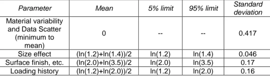
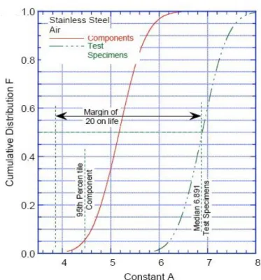
As shown in Table 1 the variation in transferability factors can differ. In order to estimate the most appropriate values, a lognormal distribution was assumed for each parameter. This allowed for a numerical statistical calculation of the total adjustment (the product of all parameters). Employing the statistical distribution of each parameter in Table 1 as input, Monte-Carlo simulations lead to an estimate of the hypothetical influence on the fatigue life when moving from a test specimen to a real life component. The natural logarithm of the factors for size, surface and load history were assumed to cover the limits 5% and 95% of the populations. In-data for the statistical analysis is summarized in Table 2. The requirement for the resulting factor on life was that the total adjustment should not compromise the failure probability of 5%. The simulation results are expressed in terms of the constant A from (1), i. e. the parameter that primarily controls the LCF region of the mean curve. The results for austenitic stainless steels are displayed in Figure 5.
Table 1: Factors on life applied to mean fatigue ε-N curve to account for the effects of various material, loading and environmental parameters.
Parameter ASME [5] ANL [1]
Material variability and Data
Scatter (minimum to mean) 2 2.1-2.8 Size effect 2.5 1.2-1.4 Surface finish, etc. 4 2.0-3.5 Loading history - 1.2-2 Total Adjustment 20 6.0-27.4
Table 2: Data for the ANL statistical analysis with log-normal distributions.
Parameter Mean 5% limit 95% limit Standard
deviation
Material variability and Data Scatter
(minimum to mean)
0 -- -- 0.417 Size effect (ln(1.2)+ln(1.4))/2 ln(1.2) ln(1.4) 0.046 Surface finish, etc. (ln(2.0)+ln(3.5))/2 ln(2.0) ln(3.5) 0.17
Figure 5: Estimated cumulative distribution of constant A in the ANL models that represent the fatigue life of test specimens and fictitious components in austenitic stainless steel. Ref. [1]
A corresponding factor on life (or margin on life) was estimated for all material types by use of these simulations. In fact, the results were quite similar for all material types and have led to the suggestion that the new design curves should have a safety factor of 12 instead of 20 on life. It should be pointed out, however, that HCF, i. e. the factor 2 on stress was never considered.
On basis of the investigation of fatigue data and margins of life, new design curves were proposed. The strategy for the generation of new fatigue curves can be summarized as follows. The mean fatigue curves are determined by finding the constants in (1) according to the strain-life data in the database. In order to establish the design curves, the mean curves are first divided by the factor 12 on life or the factor 2 on strain/stress, whichever is the most conservative. Thereafter the curves are corrected for the potential presence of a tensile mean stress, by a version of the Goodman relationship, assuming fully developed tensile mean stress. The adjusted allowable stress amplitude
adj , a
is obtained by { ( ) ( ) ( 2 )where
a denotes the non-adjusted stress amplitude,
y the yield stress and bThe difference between the previous ASME curve and the ANL curve, i. e. the current ASME curve, is considerable in the HCF regime-. In Figure 6, the ANL curve, i. e. the ASME curve since 2010, is compared with the previous ASME curves and the design curves proposed by Jaske [4]. Jaske provided curves based on the option of zero or maximum compensation for tensile mean stresses. The differences between these curves are limited in the LCF regime but become rather significant in the HCF regime. It should be pointed out that the Jaske curve with correction for mean stress and the ANL curve are in very good agreement, despite the fact that Jaske uses the factor 20 on life compared to the factor of 12 used by ANL.
Figure 6: Comparison between the previous ASME, ANL and Jaske design curves for austenitic stainless steels. Note that the ASME 2010 fatigue design curve is the same as the ANL curve.
2.1
Evaluating the ANL statistics
It is of interest to take a further look into the ANL statistical analysis in Figure 5. It is noteworthy that the shape of the cumulative distribution is almost the same for test specimen and component. In other words, the uncertainty remains unaltered when test data are transferred to a component. Mathematically, the variation in the constant A from (1) is almost the same for both the test specimen and component.
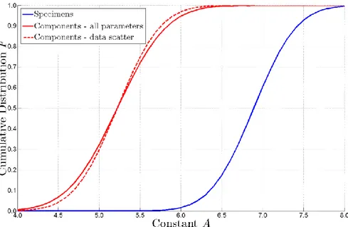
The claim that the uncertainty for a component is the same as that for the smooth test specimen is further explored. The contribution of each parameter to the uncertainty is investigated by a complementary statistical analysis. The same data and assumptions as used by ANL will be used (Table 2). In fact, by maintaining the assumption of lognormal distribution for the constant A the ANL analysis can be analytically reevaluated. By equation (3) the resulting standard deviation can be obtained.
√ ( 3 )
The test specimen value of constant A includes scatter and material variability, i. e. Sscatter whereas the component value of constant A in Figure 5 includes all scatter, Stot in accordance with equation (3). This transformation to the real component conditions can be done with and without including uncertainty for surface, size and load history. i. e, one analysis using Stot as standard deviation and one using only Sscatter as standard deviation, all other conditions the same. This will reveal how much surface, size and load history contribute to uncertainty. The results are shown in Figure 7, which contains the same cumulative distributions as in Figure 5. The additional curve is the cumulative distribution for components without consideration of uncertainty for surface, size and load history (red curve, dashed). It is obvious that the difference between the two curves for components is very small. Hence, the contribution from the uncertainty associated with size effects, surface finish and loading history, is almost negligible in terms of margin. In fact, instead of a computed factor of 12 on life in order to obtain a survival probability of 95%, only a reduction to 11 would have been required if the uncertainty of these factors were not included.
The ANL claim that the there is no increase in uncertainty when data is transferred from test data to a real component seem questionable, at least at first sight. A physical interpretation is not readily available, and a further discussion is suggested. Either there is a physical reason or the results are a fictitious consequence of the assumptions in the ANL statistics analysis. It is outside the scope of the present study to make an in-depth analysis of this complicated matter. However, the effect of load history for austenitic stainless steels on the smooth specimen level is addressed in section 4.3.
Figure 7: Reevaluation of the distribution of constant A from the ANL-model for specimens and components in air.
3.
Component testing
It is noteworthy that the document where the background for the ASME design curves is shown [2] includes component testing. This is done in order to demonstrate margins. However, all tests are done on carbon steels and no tests for austenitic stainless steels are provided.
3.1
Heald & Kiss
A recurrent reference in the literature is a series of tests performed by [6]. The series contained 15 components, straight pipes, elbows and pipes, all designed in austenitic stainless steel type 304. The tests were performed in displacement control in order to best resemble thermal loads. The tests were performed at room temperature and 288˚C. The room temperature tests included constant internal pressure. The failure criterion was related to the function of the pipe, i. e. leakage. The results for the 15 tests are shown in Figure 8 together with the ASME design curve. Notably, the load levels where computed in accordance with the formula based procedures for piping in ASME NB3600 [7]. The authors claimed the margin to be at a factor of 20 or more, but somewhat avoided to draw too general conclusions. Noteworthy is that all points lie well within the LCF regime. Hence, these much referred tests give no information about the margins in the HCF regime.
Figure 8: Resulting points from displacement controlled tests on full scale piping components in austenitic stainless steel type 304.
3.2
Marquis
Ref. [8] investigated the influence of variable amplitude loading on real components. In fact a few studies were performed on material Polarit 725 which is an austenitic material of type 304. The component consisted of a
plate with a non-load carrying, fillet welded bracket. It has been observed for many carbon steels that variable amplitude loading even at load levels well below the fatigue limit contribute to the damage. Marquis’ study gives an opportunity to evaluate this influence for austenitic stainless steel. Experiments were also carried out for a kind of carbon steel, RAEX 420, with minimum yield stress above 420 MPa.
Marquis concluded that the carbon steel showed higher sensitivity to low loads than the austenitic stainless steel. For most carbon steels, there is a well-documented tendency that loads levels below the constant amplitude fatigue limit accumulate damage under variable amplitude load. Marquis’ results show that this phenomenon may be less pronounced for austenitic stainless steel. These results could perhaps be used to derive stress reduction for welded components in piping. However, this derivation is hampered by the absence of a reliable SN-curve for stresses.
3.3
Cheng and Lu
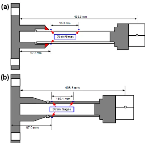
Ref. [9] and [10] have performed LCF tests on welded straight piping components of austenitic stainless steel type 304, see Figure 9. Four specimens were tested, all welded differently. The pipe specimens have a nominal diameter 31.75 mm and wall thickness 4.76 mm. The requirements were set in order to achieve the same applied bending moment at the weld toe of all specimens. Weld joint dimensions were determined according to the ASME Code. Strain amplitudes were measured about 5 mm from the weld toe. This enables a fairly direct comparison with the fatigue design curves. The geometry and resulting load cycles are given in Table 3. Results from the comparison are shown in Table 4. The predicted lives are obtained by using mean curves from Langer [2], ANL [1] and a recent curve for austenitic stainless steel type 304 [11]. It is noted that the predicted lives are always higher but covered well within a factor of 12 on life which is the design margin proposed by ANL. However, it should then also be noted that the strain gauges are placed a distance away from the cracked location. Thus, the results are not directly comparable. A correction for notch effects would alter the comparison and could probably reach increased margins. Strain amplitudes are shown in Figure 10. The strain amplitudes are rather similar for three of the specimens. However, the specimen with full sequence welding has apparently higher strain level. The reason for this difference is not analyzed in detail, but is likely to depend on different elasto-plastic conditions.
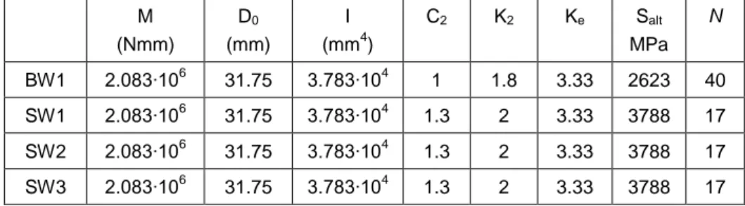
Another comparison can be obtained if ASME NB 3600 is used for analysis. This is a part of ASME III [7] that provides formula based design analysis, which is the most common way of analyzing piping systems. The end force amplitude was registered at approximately 3 kN for all specimens, which allows for the computation of the moment stresses at the location of the weld. The equations (4)-(6) are used. These data are input to the ASME design curve based on stresses. It is clear from Table 5 that there is considerable conservatism associated with this analysis.
( 4 )
( 5 )
( 6 )
Table 3: Fatigue experiment results. Ref. [10]
Table 4: Comparison between experimental results and the fatigue curves. Estimated total strain amplitude (Figure 10) Cycles to initiation Cycles to through crack ASME mean ANL Mean (ASME 2010) Colin BW1 0.65 800 980 3600 3200 6800 SW1 0.65 500 680 3600 3200 6800 SW2 0.65 560 900 3600 3200 6800 SW3 0.9 300 470 1600 1600 2500
Table 5: Comparison between experimental results and the fatigue curves.
M (Nmm) D0 (mm) I (mm4) C2 K2 Ke Salt MPa N BW1 2.083∙106 31.75 3.783∙104 1 1.8 3.33 2623 40 SW1 2.083∙106 31.75 3.783∙104 1.3 2 3.33 3788 17 SW2 2.083∙106 31.75 3.783∙104 1.3 2 3.33 3788 17 SW3 2.083∙106 31.75 3.783∙104 1.3 2 3.33 3788 17
Figure 9: Specimen geometry and strain gage locations for fatigue tests with (a) butt welds and (b) sockets welds. Ref. [10].
Figure 10: Axial strain amplitudes at fatigue crack locations from the four butt- and socket-weld experiments. Ref. [9].
4.
Cyclic plastic deformation
Austenitic stainless steels behave very differently from most other steels in the HCF regime. This is due to the rather specific elasto-plastic properties, where austenitic stainless steels will show significant plastic deformation even for long lives. The specific nature for the austenitic stainless steel can be illustrated by comparing the amount of plastic deformation for different materials for very long lives. The life chosen in this comparison is
6
10 5
N , which is typically defining the fatigue limit. It is generally assumed that negligible or small amounts of macro-level plasticity should occur for such lengthy service life. Several materials are compared in Table 6, where the amount of plasticity is shown at N 5106. Note that the austenitic stainless steel significantly differs from the others with as much as 30% plastic deformation, even though the amplitude is below the static yield limit. These results clearly show that austenitic stainless steels will show significant plastic deformation even for very long lives. The relation between elastic and plastic strain in strain fatigue over the entire load regime is shown for all materials in Figure 11 to Figure 14.
It is also of interest that the milder carbon steel also does not fully escape plastic deformation in the HCF regime. The assumption of fully linear response usually employed is obviously an idealization. However, six percent inelasticity can be claimed to be fairly small in comparison to the scatter in fatigue whereas the corresponding amount of inelasticity for austenitic stainless steel is far from negligible.
As will be shown later, the austenitic materials experience a strong history dependence upon loading due mainly to the inelastic response in all regimes. This is in sharp contrast to for example certain types of aluminum for which almost all deformation in the HCF regime is elastic and for which the load history dependence is small. Moreover, austenitic stainless steels present the characteristics of undergoing stress- or strain-induced changes at constant amplitude load, which is generally associated with what is called phase transformation. Under monotonic and cyclic loading these steels exhibit significant hardening which has been related to martensitic transformation.
Table 6: Amount of plastic deformation at the fatigue limit N5106
Material Yield stress MPa Stress at N5106 MPa Amount of plasticity % Ref. Carbon steel 1015 230 150 6 [12] Carbon steel 4340 1180 512 2 [12] Austenitic stainless steel 304 210 190 30 [11] Aluminum 2024 380 162 1 [12]
Figure 11: Strain-life data for carbon steel 1015.
Figure 13: Strain-life data for austenitic stainless steel type 304.
4.1
Secondary cyclic hardening
The considered austenitic materials exhibit a phenomenon which is normally referred to as secondary hardening at low strain levels. This phenomenon normally occurs after a large number of cycles and is preceded by a longer stage of stable stress response. Since the ASME fatigue curves are derived in strain control, and stresses are obtained by simply multiplying the modulus of elasticity this phenomenon is not directly visible in the SN-curves. As the material enters the stage of secondary hardening, the stress can increase significantly and entirely change the response. It has been previously discussed and claimed [3] that secondary cyclic hardening plays a key role for the differences in HCF data between different sources. The phenomenon has been associated with prolonged fatigue life since the amount of plastic deformation is decreased. It is believed that this effect is at least partly responsible for the difference in fatigue data between Langer and ANL. Typical examples of secondary hardening are shown in Figure 15. A central question is whether or not this phenomenon translates from specimens to real components.
The occurrence of secondary hardening is generally attributed to the effect of martensitic transformation, although other effects may contribute [13]. Colin has further noted that the onset of secondary hardening correlate well to the total accumulated plasticity. As the cumulative plastic deformation exceeds a certain level, secondary hardening is likely to begin. However, such a relation is purely empirical. An important observation by [13] is that irregular load and non-zero mean strain/stress can alter the secondary hardening. High occasional strain loads, e.g. pre-straining, may give instantaneous hardening and alteration of the microstructure. These pre-straining loads have been shown to prevent any occurrence of secondary hardening which would otherwise arise, thus also altering the fatigue behavior. These findings are clear indicators of the limits of applying constant amplitude data to real components, for which residual stresses may exist, loads are variable and cold working may pre-stain the material, effects that are all capable of altering the conditions for secondary hardening.
Figure 15: Stress response for constant strain amplitude tests presenting secondary hardening for austenitic stainless steel type 304. Ref. [13].
4.2
Effects of mean stress and mean
strain
The distinguishing elasto-plastic behavior of austenitic stainless steels has implications for fatigue. This incorporates the presence of non-zero mean strain and mean stress. Welding and surface treatment causes residual stresses and strains and constant pressure induced stresses may prevail during variation of other loads. The fatigue response under the action of mean stress therefore has relevance to nuclear piping.
The influence of secondary hardening has been discussed above. Another typical feature related to cyclic plastic deformation is ratcheting, i.e. the continuous strain increase that occurs for cyclic loading in presence of mean stress. This phenomenon is general for almost all materials. However, the presence of plastic deformation over most load ranges makes this phenomenon even more pronounced for austenitic stainless steels.
The influence of ratcheting on fatigue has been studied by [14]. The ratcheting strain and fatigue life of the material were measured at different loading levels. A dependence of ratcheting is suggested, as higher ratcheting generally leads to shorter lives where other conditions were rather similar. However, these results should be treated with some caution since it is not possible to single out ratcheting as the influencing parameter.
The existence of ratcheting in real components has been shown by [9] and [10]. Strains were measured in the set ups shown in Figure 9. The specimen SW3 was welded with full circumferential weld sequence as opposed to the other specimens which were welded with partial sequences. Initial measurements indicated a relation between strain amplitude and increased
Figure 16: Zero-shift error corrected axial strain mean values at fatigue crack locations from the four butt- and socket-weld tests. Ref. [9].
ratcheting for SW3. However, revising the measurement results leads to more ambiguous results as shown in Figure 16. The overall impression is that conclusions about the relation between strain amplitude, ratcheting and fatigue life should be drawn very cautiously. The phenomenon of ratcheting is not well understood in a quantitative sense.
Ref. [11], [13] and [15] performed analyses with different mean stress and mean strains in combination with constant amplitude fatigue loads. Fatigue data from mean strain tests are shown in Figure 17. The R-ratios of 0 and 0.75 (i.e. tensile mean strain) resulted in factors of 4 and 8 shorter fatigue lives in contrast to the fully reversed (R = -1) straining. The R-ratio of ∞ (i.e. compressive mean strain) resulted in more than an order of magnitude longer life than the fully reversed test and the specimen did not fail after more than 4 million cycles. These results are in spite of the fact that the mean stress in all mean strain tests nearly fully relaxed. Therefore, the large differences in fatigue lives observed between the different mean strain tests are merely due to the differences in mean strain. This is contrary to the common expectation that mean strain has an effect on fatigue life only if it induces a non-relaxing mean stress. Possible microstructure alterations, such as phase transformation and/or changes in dislocation structure, are discussed as explanations of this surprising behavior under mean strain (but no mean stress) conditions.
Moreover, the influence of pre-straining (PS) was investigated by [15] by pre-loading the specimens in strain control and then fatigue testing under either strain or load control. These tests were conducted with 10 PS cycles at 2% total strain amplitude. The effect of PS on fatigue life was dependent on the test control mode. PS led to significantly shorter life in strain-controlled tests (by a factor of more than 5), but significantly longer life in load-controlled test (by more than two orders of magnitude with the same stress
amplitude 275 MPa), as compared with the virgin material (i.e. without PS), see Figure 17. The results are due to the initial hardening induced by the PS. [13] propose that a damage criterion considering both strain and stress should be used in order to correlate fatigue data.
A very recent study is given by [16]. This study aims at investigating the influence of mean strain/stress in the HCF regime. Two fabrications, Thyssen (THY) and Creusot Loire Industrie (CLI), of austenitic stainless steel type 304 are investigated. Interestingly, these two fabrications show different secondary cyclic hardening behavior. For long lives, the material exhibiting the more pronounced secondary hardening (THY) had higher fatigue strength than the material (CLI) with less pronounced secondary hardening. The difference in fatigue results are shown in Figure 18. This further confirms the hypothesis that secondary hardening is a determining factor for the fatigue curve in the HCF regime with no mean strain/stress.
Figure 17: Fatigue data for constant amplitude testing. Ref. [13].
Figure 18: Strain controlled fatigue results on THY and CLI materials. Identi-fication of a strain fatigue curve (dashed line) on the THY results. Ref. [16].
4.3
Variable amplitude
Ref. [11] have performed rather detailed studies on the fatigue behavior of austenitic stainless steel type 304. Behavior under cyclic plastic deformation as well as under variable amplitude loading has been observed. The tests were carried out on smooth small specimens, with both displacement and load control. This study provides valuable information on the response of austenitic stainless steel 304 to variable amplitude loading as opposed to constant amplitude loading. Particularly, the commonly adopted strategy by using the linear damage accumulation rule (LDR) based on a fatigue design curve in constant amplitude was evaluated. Different types of load sequences were applied:
Step High-Low (H-L): Block of high loads followed by block of lower load until run-out or failure.
Step Low-High (L-H): Block of low loads followed by block of higher load until run-out or failure.
Periodic overload (POL): constant load with periodic overloads.
RL: Random loads.
Figure 19 shows a mean curve computed from constant amplitude experiments performed by [11] which is directly comparable to the ASME and ANL mean curves. In damage accumulation calculations, cycles below the fatigue limit were assumed to be non-damaging. This limit is represented by the dashed horizontal line in Figure 19.
The results from the variable amplitude loading tests are shown in Figure 20. Note that a quotient Npred/Nexp1 is an un-conservative prediction and
1
/
N
exp
N
pred is on the conservative side. From these data, the influence of spectrum load can be estimated. The influence is computed here for both the stress and strain controlled tests. It is noted that the stress controlled experiments are strongly on the conservative side in contrast to the results for strain controlled tests which are on the un-conservative side. It is furthermore noted that the nature of the spectrum has strong influence. Random spectrum for strain control exhibit far less variation than the other sequences.A direct comparison with the ANL statistical analysis of the transferability factors is made possible if the Colin quotient, ( ⁄ ) is assumed to
be lognormal distributed. Extreme values are omitted. The analysis is done for the Colin data for strain control and for all data, including stress control. The stress control data are believed to be somewhat less reliable, since no base line curve was derived explicitly for stress control. The stress control curve was derived for the strain control experiments, taking the midlife stress. Moreover, the stress control experiments are relatively few and an evaluation is not fully meaningful.
ANL performed statistical analyses to see the influence of all transferability factors, whereof variable amplitude load was considered one of them. These
calculations can be redone by replacing the ANL estimation of the variable amplitude data with the Colin data, see Table 7 for mean values and standard deviation of the logarithmic quotients (Npred/ Nexp). The resulting
transferability factors are presented in Table 8. These results are also illustrated in Figure 21, from which is seen that larger variation exists in the Colin data than reported from ANL. This means that ANL may have underestimated the uncertainty associated with loading history. In fact, the underestimation is quite large. When corrections for load history is performed with data from Colin et. al. the total uncertainty is visibly increased for the component. However, the resulting influence on the transferability factor necessary to maintain 5% is not too large, with the ANL proposed factor of 12 instead of 15 as suggested in Table 8. Hence, it is fairly likely that the relative lack of conservatism observed for strain control should be reasonably covered within the transferability factor 12, as in the current ASME. A well-judged testing program as proposed further on in this study will help to shed light on this matter.
An improvement was obtained if the assumption of strain amplitude as the only governing parameter was abandoned. Alternatively, a criterion by [17] (SWT) was used which instead employs a parameter that consists of the product between the maximum stress and strain amplitude, maxa. This empirical criterion considers hardening effects associated with the elasto-plastic properties and correlates the data better. This improvement is the most significant in the High-Low sequence and the least under random load. The overall improvement can be seen in Figure 22. It is noted that this correction applies successfully for all load ranges.
Table 7: Mean values and standard deviations for spectrum loads.
Mean value Standard deviation ANL 0.438 0.160 Colin Strain control1) 0.492 0.371 Colin all data1) 0.244 0.585
Table 8: Reconsidered influence of variable amplitude on number of cycles.
ASME 20 ANL 12 Colin Strain control1) 15 Colin All1) 15
Figure 19: Fatigue curves based on constant amplitude testing.
Figure 20: Quotient between predicted and experimental life for different types of loading sequence.
Figure 21: Cumulative distributions for data from ANL and data from Ref. [11] for which strain control alone and both strain plus load control are illustrated.
Figure 22: Predicted versus experimental lives for stainless steel type 304 using the Palmgren-Miner linear damage rule (a) without and (b) with the SWT parameter. Ref. [11].
5.
Surface Roughness
It is noteworthy that both Cooper [5] and ANL [1] have pointed out surface finish as the largest transferability factor from a smooth test specimen. In fact, ANL suggests that this effect is more pronounced for austenitic stainless steels than carbon steels. They claim that the surface finish effect is reduced for carbon steel in LWR environment, whereas this effect may be maintained for austenitic stainless steels.
Fatigue cracks are in most cases initiated at the surface of structural components. The crack initiation times could potentially be reduced by an increased surface roughness as this geometrical state may serve as a catalyst for premature crack initiation. Materials whose fatigue life is dominated by the crack propagation stage are less sensitive to the topography compared to materials whose fatigue life is dominated by crack initiation.
Different degrees of surface roughness are illustrated in Figure 23. A reduction in fatigue life due to increased surface roughness alone can only be expected when the crack initiation occurs at the base of roughness grooves rather than at material weaknesses such as slip bands and grain boundaries. An elaborate discussion can be put forth regarding the influence on fatigue life depending on the relation between surface roughness, grain size and operation temperature. Results indicate that the crack initiation sites for specimen with rough surface are changed gradually from the surface grooves to grain boundaries as temperature and grain size are increased. Four example specimens are presented in Figure 24. There is a certain degree of disagreement between results from LCF experiments in the literature as some observe a reduction of total fatigue life while others do not. It is further unclear to what extent the increase of surface roughness that has developed during fatigue loading in an initially smooth specimen affects the fatigue life [18].
From LCF-experiments performed at 593˚C, it has been observed that surface finish can have a significant influence on the life of specimen made of stainless steel types 304 and 316. This appears to be the case in particular when transverse flaws (orthogonal to the loading direction) are considered. Longitudinal flaws (parallel to the loading direction) had much less detrimental effect on the fatigue life and were therefore not discussed in detail. For transverse flaws, it was seen that the number of load cycles to initiate a crack was clearly reduced with an increase in surface roughness. Crack initiation for a smooth specimen at a strain range of 1% dominated 70% of the total fatigue life. A surface roughness R=2.9µm reduced the total fatigue life by a factor of two [19].
Effects of surface passivation and electropolishing on a group of biomedical stainless steels of type 316 were investigated. The treatments proved to have a significant effect on the final surface finish although static mechanical testing revealed no difference in the static mechanical properties regardless of surface treatment. Tests were carried out in both air and wet environments. The tests in air revealed that electropolishing performed best
in terms of fatigue performance and that electropolishing followed by passivation did not perform much better than electropolishing alone [20]. A concern has been raised regarding the measure of the surface roughness and whether the observed impact can be isolated to the topographic characteristics alone or if the large scatter in the literature for equal roughness values to some extent should be attributed to mechanical impact due to the surface roughness manufacturing. More recent models for characterizing surface roughness have recognized that measures relating to maximum irregularities are better indicators rather than average values [21].
Figure 23: SEM micrograph photos and surface roughness profiles of type 304 stainless steel specimen. The maximum difference in peak to valley height for the pictured examples are (a) Rmax=13.0µm , (b) Rmax=0.3µm and
Figure 24: Type 304 stainless steel specimens with a rough surface were tested at 600˚C. SEM micrograph photos showing specimens with (a) 50µm grain size and Rmax=13.0µm, (b) 50µm grain size and Rmax=0.3µm, (c)
500µm grain size and Rmax=13.0µm and (d) 500µm grain size and
Rmax=0.3µm. Only (a) displayed crack initiation sites at the surface grooves
6.
Welds
It is to be noted that the influence of welds has not been considered in any previous discussion on margins performed by ANL [1] or [5]. This appears as a limitation since welds has been a primary concern in other modern standards [22], [23] and [24], which deliver quite detailed information on how to account for welds.
The introduction of welds contributes with many questions and concerns regarding the influence on the fatigue life of the specimen or component. Not only does the weld pose the risk of unfavorable geometry from its irregular shape, it may also introduce flaws which could partially or even completely eliminate the crack initiation process. Most studies of weld fatigue have been executed on ferritic materials for which the total fatigue life is dominated by crack propagation. This becomes an important issue for materials that behave differently as the crack initiation process can be strongly influenced by changes in material properties in contrast to the crack growth rate that may not. In cases where the final weld does not involve pre-existing cracks (defects beyond a certain tolerance), the welding process inevitably introduces unfavorable residual stresses. Without post weld heat treatment, it is not uncommon for the tensile residual stresses to be of the same order as the yield point.
Access to an extensive library of data collected from a large number of sources has served the foundation for a relatively extensive analysis of weld fatigue. Welded and unwelded specimens, plates and joints covering a large variety in e.g. temperature and weld techniques were tested and the results exhibit a large scatter, see Figure 25. The results scatter for HCF-experiments including e.g. the effect of R-value, surface roughness and weld technique appears on both sides of the ASME design curve (prior to 2010) and the ANL design curve (ASME 2010). The data points fall on both sides of the design curves which for two reasons may not be as alarming as it first appears. Firstly, the experiments were performed with stress controlled loading which, as has already been pointed out, leads to results on the un-conservative side compared to the design curve. Secondly, fatigue reduction factors for the stress concentration at welds have not been included which if employed could further account for the deviation, ref. [25].
Figure 25: Data points from a large variety of load controlled tests performed on austenitic stainless steel where e.g. the presence of welds, welding method, R-value and surface roughness display a relatively pronounced scatter.
7.
Discussion
The presence of documented LCF and HCF fatigue experiments performed on full scale industrial components made from austenitic stainless steel types 304 and 316 in the literature is scarce. A few experiments in LCF were conducted in the 1970s and earlier and appear to be recurring sources in the available literature. It is often the case that a lack of statistical redundancy and duplicate tests constrain the reliability of any general conclusion. Hence the data should be regarded as spot checks of margins rather than solid evidence. However, these spot checks so far do not point at any potential lack of conservatism in ASME.
More troubling is that reliable HCF data seem almost impossible to find in the common literature. Such data should be mandatory to clarify the concerns about ASME margins in for HCF which has been caused in conjunction to the discussion about the ANL design curve proposals. The ANL design curve is based on test results from small, smooth specimen loaded in constant strain amplitude. It has been readily shown in this study that smooth specimen tests with constant amplitude is a special case, providing very little information about real margins. The necessity to move on to tests under much more realistic conditions is emphasized.
Since the literature offers a restricted documentation of experiments on component level, the literature search transformed into studying research on four observed phenomena separately for the material under consideration. The selected phenomena are (a) cyclic plastic deformation, (b) surface roughness, (c) welds and (d) variable amplitude.
Austenitic stainless steels display a large plastic deformation hardening during cyclic loading. Experiments have shown that strong history dependence exists while there is a particularly pronounced difference between the cyclic stress-strain curve and the monotonic stress-strain curve for stainless steels compared to other materials. It is believed that the plastic deformation behavior is an important key to understanding the transferability. It is however assumed that this strong dependence does not require tests designed to capture the plastic deformation behavior in particular. The reason is that this kind of behavior is inevitably present in all tests that could be of interest in this study.
Observations show that surface roughness does act detrimentally on the crack initiation part of the total fatigue life. The reliability of results in experiments where surface roughness is being manufactured has been questioned in the literature as the machining may be influential in terms other than only surface topography, e.g. residual stress. There is also some disagreement in the literature concerning the circumstances under which the crack nucleation is located in the roughness grooves rather than at intrinsic weaknesses of the material.
The introduction of welds may result in a fairly large degree of uncertainty due to the risk of introducing pre-cracks into the structural component. This could potentially eliminate the entire crack initiation phase of the total
fatigue life which would greatly reduce the fatigue life. Other less harmful encounters include geometrical detriments and material transformations. Variable amplitude loading has a fundamentally different significance for the fatigue life compared to constant amplitude loading. Constant amplitude loading could be thought of as a special case of random loading and should also be treated as such. Austenitic stainless steels display a strong dependence on the loading sequence due to the elastic-plastic material properties. Most industrial applications call for an increased understanding of the influence related to random loading.
The possibilities in investigating transferability are extensive and must be reduced to a selected set of parameters which are of particular interest. This approach is necessary due to the in some sense infinite number of possible component configurations. Real components suffer from connecting all the different parameters into a combined effect on the fatigue life. Isolation of each parameter’s influence is therefore crucial in order to establish an understanding that can be applied to a large range of structural components and configurations. Based on the literature search, welds and variable amplitude loading are considered to be the two most important among the four selected phenomena in the above. It is believed that a carefully planned experimental scheme with a particular interest in welds and variable amplitude loading can bring further light on the actual margins between design curves and the true fatigue life for a larger range of components. Proposed experimental setup consists of a four point bend configuration of a welded pressurized straight pipe. The FPB thus enables the testing of a realistic component. Variability of configuration is obtained since both welded and unwelded sections can be tested. In the longer perspective, the influence of different weld quality and the influence of surface treatment can be investigated. It is considered important that variable amplitude is applied in the test setup.
There are several options available when determining a failure criterion, e.g. leakage and reduction of stiffness. Independent from which is chosen, it is important that the detectability is appropriate in order to minimize the results scatter related to the selection of failure criterion. Piping systems are typically design to contain a transported medium and keep a specific internal pressure. For such a component, monitoring the feeding and applied internal pressure may be an appropriate criterion which is also closely connected to the structural intent of the component.
Details and further argumentation with regards to the proposed experimental set-up is given in section 9 in this report. These experiments aim at significantly improve the knowledge about margins in the ASME fatigue design procedure, which is much needed. In fact, this improvement can be obtained within moderate effort by choosing the relevant conditions for the experimental evaluation.
8.
Conclusions
The margins in the ASME fatigue design procedure for austenitic stainless steel have been evaluated in this report. The evaluation has been based on a literature search in order to find relevant data and data on component testing in particular. Some conclusions have been drawn during the study on both areas, see below.
The following conclusions can be drawn:
1. The very small number of existing data on component testing in austenitic stainless steel shows satisfactory margins. These data come almost exclusively from low-cycle fatigue (LCF) tests with constant amplitude.
2. Very few component data for high cycle fatigue (HCF) exist which is a shortcoming. The major discussion on ASME margins is due to the significant difference in HCF data between Langer and ANL data.
3. Secondary cyclic hardening is decisive for HCF in constant amplitude testing in strain control. The effect of this phenomenon is likely to be altered under variable load.
4. Secondary cyclic hardening behavior may differ between batches from different manufacturers.
5. HCF for austenitic stainless steels is determined by its complex elasto-plastic behavior also in the HCF regime.
6. The control mode, load or displacement, is important for fatigue. 7. It is shown that using strain amplitude as the only fatigue governing
parameter is inaccurate. A better agreement is obtained by using combined measures involving both stress and strain.
8. Discussions about high cycle fatigue margins in ASME cannot be based on HCF data for fully reversed strain load on small smooth specimens as has been done by ANL. Relevant component testing is simply necessary where conditions for elasto-plastic deformation must be realistic.
9. Welds and surface conditions significantly affect the fatigue life. However, available data shows great variation.
10. A testing program for pressurized straight pipes loaded in four point bending is proposed.
11. The testing should be performed with variable amplitude and with enough points in order to establish prediction limits, thus enabling comparison with margins in ASME. This is highly recommended.
9.
Proposed experimental
set-up
An experimental investigation will be proposed and outlined in this section. It is of importance that the testing conditions are as realistic as possible and that the tests give information about margins in ASME that are general and not only valid for a specific case. Moreover, the results should be obtained without an excessive number of testing specimen. Here are some of the key parameters that should be observed, so that the scope can be obtained within reasonable effort:
Variable amplitude, with load spectra relevant for nuclear piping.
Realistic welded piping component or part, manufactured in compliance with nuclear requirements.
Realistic failure criteria, i. e. leakage or wall penetration.
Experimental results expresses as an SN-curve.
Statistical treatment in order to establish predictions limits, i. e. a design curve.
Possibilities to compare the experimental results and ASME in the same diagram.
In order to obtain SN-curves, both mean and design, under variable loading some assumptions must be made. The most important assumption is to postulate the linear damage accumulation rule. In fact this is no limitation since the ASME procedure is based on the assumption that the linear damage accumulation rule applies, e.g. the Palmgren-Miner rule [26] and [27]. The damage rule is expressed as a sum of the damage contribution at each load level included in a load sequence. The constant amplitude design curve serves as scale factor for the damage contribution from each load level. The condition for failure is that the total accumulated damage D reaches a specific value (usually unity) and can be expressed as
∑ ( 7 )
where ni are the number of cycles at a specific load level and Ni is the
corresponding fatigue life as returned by the constant amplitude design curve.
It has been concluded elsewhere in this report that a combined measure such as the SWT-parameter is better than using strain amplitude alone as the fatigue governing parameter. However, the proposed testing program should still use strain in order to maintain comparability with ASME and thus arrive at a relevant evaluation of margins in the standard procedure.
An SN-curve is required to apply the linear damage rule. Let’s begin with a curve intended for constant amplitude loading which is assumed to be linear in its logarithm form
( 8 )
where N is the number of cycles to failure, is the strain amplitude and A and B are unknown constants to be determined. It is possible to replace the strain amplitude by an equivalent strain measure computed from a variable amplitude load sequence. The equivalent strain should return exactly the same total damage as the entire sequence. Based on these assumptions, the equivalent strain can then be uniquely expressed as
(∑ )
⁄
( 9 )
where is the strain level at each load level of the sequence and is the total number of load cycles during the entire load sequence. It is a rather straightforward task to make a log-log best fit of data according to the equivalent strain as defined in (9) against the number of cycles to failure. This is done by employing a numerical iterative scheme to determine the constants A and B in (8) where ahas been replaced byeq.
Appropriate confidence intervals and predictions limits can be computed, thus enabling the establishment of a design curve. For the direct and convenient evaluation of ASME margins it is possible that the above scheme should be altered somewhat. Based on (9), a modified equivalent strain can be defined. The curved part, i.e. the curvature introduced by the constant C in (1), is essential in the discussion about margins in ASME margin. The correction of the equivalent strain should then read
(∑ ( ) ) ⁄ ( 10 )
The task is now to determine the constants A, B and C in such a way that a best fit is obtained in (8), i.e. linear in the log-log diagram. The constant C can be interpreted as a kind of cut-off limit for fatigue damage. Note that by input of the constants in (1) a direct comparison with both the ANL-curve and the ASME curve is possible. Determining the constants A, B and C can be seen as an inverse determination of the SN-curve. In fact, as this base curve can be experimentally determined, a comparison with the ASME design curve can be made directly in the same diagram. Confidence intervals and prediction limits can be readily established, thus creating a design curve that is directly comparable to the ASME curve,
A detailed description of the above introduced creation of SN-curves from spectrum tests is given by [28]. An example of how to fit spectrum data to a straight line in the log-log diagram is shown in Figure 26. Note that run-outs
are included, and that relatively few tests are needed to establish prediction limits. The prediction limits include 90% probability, enabling the establishment of a design curve at 5% failure probability. It is noteworthy that the 5% limit is exactly the same as proposed by ANL.
It has been concluded that experiments on components or realistic specimens would contribute significantly to an increased understanding of the ASME margins. Moreover, developing and establishing a useful testing technique has the possibility for future use. It is not unlikely, that there will be occasions when there is a need to for example compare different testing techniques, measure residual stress redistribution etc.
Four-point-bending (FPB) is a convenient technique for straight component testing. This provides a robust way of obtaining a constant nominal load over a larger length. The set-up shown in Figure 27 has the advantage that a realistic pipe section can be tested. The pipe specimen may or may not contain a weld of arbitrary condition. Hence, the possibility to test the influence of the weld condition is available. It is comparatively difficult to obtain reversed load with FPB, i. e. R<0. However, this is not a significant limitation, since always testing with R≥0 secures tensile mean loads. This makes sense, since the ANL proposed design curve is intended to account for the effects of high tensile stresses. Thus, results from such testing would be more easily comparable to the ANL design curve. Moreover, modern codes such as the IIW recommendations [23] usually employ high mean stress in fatigue testing of welds.
Figure 26: A load norm for spectrum load (equivalent stress) is fit to a linear expression in the log-log curve. Prediction limits at 90% are given. (Courtesy SP Technical Research Institute of Sweden.)
Figure 27: Principle of a FPB set-up for a pipe section under displacement control.
A remaining question is whether the pipe section should be subjected to internal pressure or not. An internal pressure would create a multi-axial constant stress state, with stresses in the circumferential and axial direction. This also helps introducing a realistic failure criterion, namely leakage. The tests should be performed primarily by displacement controlled loading in order to make the results comparable to the ASME results. Strains could be locally measured and an optical technique, e.g. speckle measurements, which would be beneficial since then both local and nominal strains could be measured. Otherwise, measuring strains with conventional technique will also be possible. Tests performed as described above will include the influence of some key parameters listed below, which are not included in the tests of small and smooth specimen. The proposed set-up is universal and has the potential for even further studies, where the individual parameters can be studied in detail. The parameters of interest can also be varied in magnitude or combined in different constellations in order to single out the influence from each individual parameter. The key parameters are
Size
Surface condition
Multi-axial load states
Mean stress/strain
Variable amplitude
Weld
Failure criterion
In summary, the above proposed tests constitute a flexible and convenient way of significantly improving the knowledge about margins in ASME. The proposed study should be performed in the first place on welded pipes since welds are common fatigue initiation sites. Performing these tests is strongly recommended.
10.
References
[1] O.K. Chopra and W.J. Schack, "Effect of LWR coolant environments on the fatigue life of reactor materials," 2007.
[2] ASME, "Criteria of the ASME Boiler and Pressure Vessel Code for Design by Analysis in Sections III and VIII, Division 2," New York, 1969.
[3] J. Strömbro and M. Dahlberg, "Evaluation of the Technical Basis for New Proposals of Fatigue Design of Nuclear Components," 2011. [4] C.E. Jaske and W.J. O'Donnell, "Fatigue design criteria for pressure
vessel alloys," Transactions of the ASME Journal of Pressure Vessel Technology, pp. 584-592, 1977.
[5] W.E. Cooper, The Initial Scope and Intent of the Section III Fatigue Design procedure, January 20-21, 1992.
[6] J. Heald and E. Kiss, "Low cycle fatigue of nuclear pipe components," Journal of Pressure Vessel Technology, pp. 171-176, 1974.
[7] ASME, "ASME Boiler & Pressure Vessel Code, ASME III Division 1, NB-3000," 2007.
[8] G.B. Marquis, "High cycle spectrum fatigue of welded components," 1995.
[9] P.Y. Cheng, "Influence of Residual Stress and Heat Affected Zone on Fatigue Failure of Welded Piping Joints," North Carolina State University, 2009.
[10] X. Lu, "Influence of residual stress on fatigue failure of welded joints," North Carolina State University, 2002.
[11] J. Colin and A. Fatemi, "Variable amplitude cyclic deformation and fatigue behavior of stainless steel 304L including step, periodic and random loadings," Fatigue & Fracture of Engineering Materials & Structures, pp. 205-220, 2010.
[12] S. Suresh, Fatigue of Materials. New York: Cambridge University Press, 1991.
[13] J. Colin, A. Fatemi, and S. Taheri, "Cyclic hardening and fatigue behavior of stainless steel 304L," Journal of Materials Science, pp. 145-154, 2011.
[14] G. Kang, Y. Liu, and Z. Li, "Experimental study on ratcheting-fatigue interaction of SS304 stainless steel in uniaxial cyclic stressing," Materials Science and Engineering, pp. 396-404, 2006.
[15] J. Colin, A. Fatemi, and S. Taheri, "Fatigue behavior of stainless steel 304L including strain hardening, prestraining and mean effects," Journal of Engineering Materials and Technology, pp. 1-13, 2010. [16] L. Vincent, J.C. Le Roux, and S. Taheri, "On the High Cycle Fatigue
behavior of a type 304L stainless steel at room temperature," International Journal of Fatigue, p. To appear, 2011.
[17] K.N. Smith, P. Watson, and T.H. Topper, "A Stress-Strain Function for the Fatigue of Metals," Journal of Materials, pp. 767-778, 1970.


![Figure 4: The ASME mean curve and the so-called Langer data. Ref. [2] The ANL report [1] also performed a thorough review of the transferability factors of 2 on strain/stress or 20 on cycles](https://thumb-eu.123doks.com/thumbv2/5dokorg/3346951.18860/12.892.200.680.590.875/figure-langer-performed-thorough-transferability-factors-strain-stress.webp)