Mining, Economic Activity and Remote Sensing:
Case studies from Burkina Faso, Ghana, Mali and Tanzania
4Magnus Andersson
1Ola Hall
1Niklas Olén
232015-02-03
Abstract
Mining is a major economic activity in many developing countries particularly in Africa. Mining operations, whether small- or large-scale, have an impact on local communities. Previous research focus on how the gold mining sector
in Africa is dependent on policy reforms in order to enable countries to better benefit from the sector, changing environmental conditions or the structure of the economic activities in the areas surrounding mines. Here, we apply a
novel analytical framework based on medium resolution satellite data for the period 2001 – 2012 to estimate the economic effects of mining in Ghana, Mali, Burkina Faso and Tanzania. Through the analysis of nighttime lights, agricultural vegetation dynamics and forest change, we find a positive effect on average economic growth for most mining districts in Mali, Burkina Faso and Tanzania. Moreover, our analysis establishes strong relationship between
statistics of agricultural production and vegetation index from satellite data on district level in Mali, Ghana and Tanzania.
1 Department of Human and Economic Geography, Lund University, Sölvegatan 10 SE-223 62 Lund, Sweden tel: +4646 2220000, e-mail: magnus.andersson@keg.lu.se
2 Department of Physical Geography and Ecosystems Analysis, Sölvegatan 12, SE-223 62 Lund, Sweden
4 We acknowledge the contributions of Anja Tolonen who conducted the econometric analysis, Punam Chuhan-Pole, Andrew Dabalen, and Aly Sanoh and the participants at Mid-Term Review Workshop on Socioeconomic Impact of Gold Mining on Local communities organized by the Office for the Chief Economist on Africa, World Bank on May 29 2014 in Washington DC. Special thanks go to Likki Lee, Prince Young Aboagye, Maria Francisca Archila Bustos, Eigo Tateishi, Bastian Berlin and Antonio Kusbach, graduate students at Lund University for excellent research assistance.
1
1. Introduction
Mining is a major economic activity in many developing countries particularly in Africa (Weng et. al 2013). Mining operations, whether small- or large-scale, have an impact on local communities. Previous research focus on how the gold mining sector in Africa is dependent on policy reforms in order to enable countries to better benefit from the sector (Gajigo et. al 2012), changing environmental conditions or the structure of the economic activities in the areas surrounding mines (Hilson 2002). Three major factors have been highlighted in relation to the main challenges facing the African mining industry. Low levels of expenditure on exploration and weak downstream processing providing low industrialization of the industry. Many countries are dependent on export earnings from the mineral sector thus vulnerable for external shocks and even despite years of efforts to improve the sector´s competitiveness it have not yet been translated in sustainable economic growth (Hilson 2014). Thirdly, in some African countries, environmental problems and social issues caused by mining have been sources of protests and conflicts between mining companies and communities in mining areas (Campbell 2012). Mining has often been associated with deforestation, land degradation, air pollution, and disruption of the ecosystem (Hilson and Yakovleva 2007).
The aim of this proposed research is to gain a better understanding of the socioeconomic impact of resource extraction on local economic growth with a focus on agricultural production. One important outcome of interest is whether the opening of mines has spillover effects on economic activities within the agricultural sector. Agricultural production could be affected by mining activities in several ways. Mining could lead to a rise in local wages, reduce profit margins in agriculture and lead to exit of many families from farming a localized Dutch disease problem. Negative environmental spillovers such as pollution or local health problems could also dampen productivity of the land and the farmers. Alternatively, mining could create a mini-boom in the local economy-that is, higher employment and higher wages can lead to an increase in local area aggregate demand, including for regional food crops.
The objective of this study is to use remote sensing data to estimate level and growth (or decline) of economic activities in reference to the mining industry in Burkina Faso, Ghana, Mali and Tanzania by comparing estimated levels and changes in agricultural and non-agricultural production in mining and non-mining localities. A selection of radius around the mining areas has been developed in order to estimate the level and composition of production – agricultural and non-agricultural – as a function of distance from the mining areas.
Our study identified 32 mines within the studied countries as prime study areas. A total of 8 mines (2 per country) were chosen to be reported in the analysis. This paper contributes to the literature by studying the effects of natural resources on development using remote sensing data. Moreover, our study investigates the spatial relationship between mining activities by using a vegetation index as a proxy for agricultural production.
Our study is divided into two parts. Firstly, we use time-series analysis of remote sensing data from three different sources in order to estimate change over time in the area surrounding the mines. Nighttime light data from the National Oceanic and Atmospheric Association’s National Geophysical Data Center (NOAA-NGDC) are used to identify artificial light emissions and has previously been used to estimate growth in economic activities. Recent studies conducted by economists have paid attention to human generated night-time light data and tried to associate these with economic growth in order to overcome estimation errors (Elvidge, et al. 1997) (Sutton and Costanza 2002) (Doll, Muller and Morley 2006) (Ghosh, et al. 2010); (Henderson, Storeygard and Weil 2012) (Ebener, et al. 2005) (Chen and Nordhaus 2011). The second data source related to vegetation changes play an important role in the environmental 2
processes, and is also a sensitive indicator for environmental and global changes (Van Wijngaarden, 1991). The vegetation monitoring can provide useful clues concerning our changing environment and help natural resource management. Traditional method to monitor the vegetation is by field investigation. It is low efficiency and high labor demanding, especially for large scale area, and impossible to conduct continuously. Time-series analyses of satellite data enable the observation of seasonal and annual trends of vegetation cover (Vicente et al, 2004). Our study test the relationship between vegetation index and the actual agricultural production reported by the National Statistics offices in Tanzania, Ghana and Mali by using geographically weighted regression (GWR). Su et al. (2001) pointed out that the results or conclusions for the same area may change with different spatial resolution of research scale. And it is important to understand the effect of different resolution images on the analysis of spatial variation. The selection of radius around the mining areas estimates change of time for 10, 20, 30, 40 50 and 100 kilometers from the mine. Secondly, we look at estimated growth in economic activities on district levels in the studied countries to evaluate growth patterns in districts with a mine, districts neighboring a district with a mine and other districts that are not close to a mine.
The rest of the paper proceeds as follows. The next section. 2 provides a summary of the methods and data used in the study. Section 3 reviews the literature on remote sensing and economic activities with particular focus on agriculture. Section 4 includes the results from the analysis of the mining sites and the economic growth model on district levels. Section 5 estimates if night lights, greenness and forest coverage change in mining communities with mining onset, we employ an empirical estimation strategy called difference-in-difference (previously employed to understand the economic effects of gold mining in Africa by Aragón and Rud (2013), Tolonen (2015), and Kotsadam et al., (2015). Section 6 concludes the paper.
2. Methods and Data
Since the early days of satellite remote sensing, its accessibility, quality, and scope of have been continuously improving, making it a rich data source with a wide range of applications (United Nations, 2014). Although there are a few examples of remote sensing to be found in the social sciences, developments have, on the whole, been less pronounced (Hall 2010). With the advent of new medium resolution remote sensing datasets with global coverage this is about to change. Here, we apply a recent framework based in the work of Henderson (2012) and extended by this group (Keola et al., 2015). In that study we performed estimations of economic activities on global, national, and subnational levels with a focus on developing economies using remote sensing data. Further, it extended the recent statistical framework using nighttime lights to augment official income growth to account for agriculture and forestry which emitted less or no additional observable nighttime light. In the study we argued that nighttime lights alone may not explain value-added by agriculture and forestry. By adding land cover data, our extended framework could be used to estimate economic growth in virtually all administrative areas of any sizes.
With that said, the limitations of most global land cover data products are severe (McCallum et al, 2006). Land cover data is conceptually similar to maps and nominal to its character. Classes are derived through a classification process and overall accuracies are generally low. Furthermore, land cover classification is a tedious and expensive process and therefore the temporal resolution becomes very low. This is particular true for large area mapping such as regional and global land cover data sets.
Here, we further elaborate on the framework by (Keola et al., 2015) by abandoning traditional land cover data in favor of MODIS NDVI which is a global continuous dataset suitable of studying vegetation dynamics at high spatial and temporal resolutions. Our study provides a spatial analysis of the relationship between NDVI and actual agricultural production on districts levels. We find a strong association between actual production of agricultural products and NDVI using spatial regression. An important difference between spatial and traditional (a-spatial) statistics for example OLS regression is that spatial statistics integrate space and spatial relationships directly into their mathematics. Spatial regression methods capture spatial dependency in regression analysis, avoiding statistical problems such as unstable parameters and unreliable significance tests, as well as providing information on spatial relationships among the variables involved. Depending on the specific technique, spatial dependency can enter the regression model as relationships between the independent variables and the dependent, between the dependent variables and a spatial lag of itself, or in the error terms. Geographically weighted regression (GWR) is a local version of spatial regression that generates parameters disaggregated by the spatial units of analysis. This allows assessment of the spatial heterogeneity in the estimated relationships between the independent and dependent variables.
For each districts, a regression coefficient can be estimated using a GWR model (Fotheringham et. al., 2002 and Lloyd for empirical examples ). GWR method allows for analyzing the spatial variability of the local coefficients of the independent variable and can explain spatial heterogeneity. OLS creates a regression coefficient which assumes that the relationship between the studied variables is constant across the landscape. GWR assumes that the relationship between NDVI and the total agricultural production may vary over space.
We also include the recent dataset on forest change by Hansen (2013). Below we present our four datasets and how they were processed. In addition, data has after processing been assembled into a geodatabase with the working title “African Economic Growth, light and vegetation database” (AEG, 2014).
Nighttime Lights
Nighttime lights data from the National Oceanic and Atmospheric Association’s National Geophysical Data Center (NOAA-NGDC) was used. Since the mid-1970s, NOAA-NGDC has operated the Defense Meteorological Satellite Program’s Operational Linescan System (DMSP-OLS) and has digitally archived the imagery since 1992 (Baugh, et al., 2010). The sensors are flown on a sun-synchronous, low altitude, polar orbit and are designed to collect global cloud imagery (Baugh, et el., 2010; Elvidge, et al., 2009b; Elvidge, et al., 2004). The sensors have a resolution of 0.56 km; however, on-board averaging of this data into five by five blocks produces a “smoothed” dataset with a resolution of 2.7 km (Baught, et al. 2010; Elvidge, et al., 1999). Each sensor collects 14 orbits daily in 3000 km swaths which provide for complete global coverage four times during the day at dawn, daytime, dusk and nighttime (Elvidge, et al., 2009b; Elvidge, et al., 2004). At night, the visible band is intensified using a photomultiplier tube (PMT), which allows the sensors to detect clouds illuminated by moonlight (Baugh, et el., 2010; Elvidge, et al., 2009b; Elvidge, et al., 2004). The PMT boosts the detection of light and so allows the detection of lights such as human settlements, gas-flares, fires, fishing boats and the aurora (Baugh, et el., 2010; Elvidge, et al., 2009b; Elvidge, et al., 2004).
At a minimum, one satellite is operated each year. However, as the satellites and sensors age, the quality of data produced decreases and they must be replaced. In most years, there are therefore two satellites collecting data (Elvidge, et al. 2009b). The NOAA-NGDC produces three annual nighttime lights products from this data which are freely available to the public: cloud-free, average visible lights and stable lights composites. Additionally, a radiance calibrated and an average lights x pct dataset are produced from this data4.
For this analysis, the annual stable lights composite (version 4) was used (NOAA-NGDC, 2014a).It provides data on the average visible band digital number (DN) values for all cloud-free observations. The DN values range from 0 to 63 and correspond with the brightness of the observed lighting (NOAA-NGDC, 2014b). It is filtered to remove ephemeral lights and background noise (such as auroras, forest fires, lights from fishing vessels and reflections of moon or starlight) so that only persistent surface lights remain (Elvidge, et al., 2013). A series of algorithms are used to select the best data to include within the composite image and the data is reprojected into 30 arc-second grids, between the latitudes of 65° S and 75° N (Baugh, et al., 2010). Baugh, et al. (2010) provides an in depth explanation of the processing required to generate the stable lights composite. The stable lights dataset was selected because it provides a worldwide view of human development from space. It is versatile in that the sensors are able to detect faint light sources from rural areas as well as bright lights from urban areas and, since it contains DN numbers, differentiation between different types of light sources can be made (Elvidge, et al., 2013). Furthermore, it is consistently available on a yearly basis, which is not the case with many of the other nighttime lights products.
MODIS NDVI
Normalized difference vegetation index (NDVI) from MODerate Imaging Spectroradiometer (MODIS) vegetation indices product MOD13Q1 were used (ORNL DAAC, 2011). The NDVI data is provided as a global dataset with a 16 day temporal resolution and a spatial resolution of 250 m. NDVI is dimensionless
4 See NOAA-NGDC, 2014b for a description of each of these datasets
5
spectral index that relates to the photosynthetic uptake by vegetation (Myneni and Williams, 1994; Sellers, 1985). It is calculated from the near infrared (NIR) and red wavelength bands by using the following relationship:
NDVI = (NIR – Red) / (NIR + Red)
It has previously been shown that NDVI is related to, for example, the vegetation greenness, leaf area index (LAI), and primary productivity of the vegetation (Johnson, 2003; Paruelo et al., 1997). It has, furthermore, been shown that NDVI time series can be used to assess the changes in vegetation cover and responses over time (Hill and Donald, 2003) and that it can be used to estimate agricultural yields (Labus et al., 2010; Ren et al., 2008). This makes it possible, by using remotely sensed NDVI, in regions where field data are sparse, on a large scale, evaluate the vegetation status and the agricultural productivity.
MODIS NDVI processing
Since the MOD13Q1 product, for each time step, is acquired as a Hierarchical Data Format (hdf) file it was converted into a raster data format (.rst) that was needed further on in the processing. The 16-day converted NDVI data were, per pixel, filtered and the yearly amplitude were extracted by using TIMESAT. TIMESAT is a specialized software designed to extract information from remotely sensed vegetation time-series (Eklundh and Jönsson, 2012). This was done by, first creating a file list, text file, specifying the location and order of the raster files. Secondly, a TIMESAT settings file was created which pointed to the previous created file list, defined the output and the filtering method, in this case a Savitzky-Golay filter. By running TIMESAT with the created settings file an output file with the filtered data was created. Finally, the yearly amplitude was for each pixel extracted from the filtered data by taking out the difference between the yearly minimum and maximum value. In the case that the peak growing season occurred during Nov-Feb the calendar year was allowed to be flexible. This since a complete growing season must be selected to be able to extract an amplitude value.
Finally, a mask was constructed to exclude land covers that are not part of the agricultural economy. For this purpose, the MODIS Land Cover Type product (MCD12Q1) was used (Friedl et al., 2010). As such, it contains five classification schemes, which describe land cover properties derived from observations spanning a year’s input of Terra- and Aqua-MODIS data. The primary land cover scheme identifies 17 land cover classes defined by the International Geosphere Biosphere Programme (IGBP), which includes 11 natural vegetation classes, 3 developed and mosaicked land classes, and three non-vegetated land classes. Here, desired classes from the IGBP classification were Croplands (#12) and Cropland/Natural vegetation mosaic (#14). For classes #12 and #14 Sum of NDVI Amplitude was calculated in the same manner as above.
Gross Forest Loss
The recent global dataset of Hansen et al (2013) was used to quantify forest loss annually. They have mapped global tree cover extent, loss, and gain for the period from 2000 to 2012 at a spatial resolution of 30 m. The dataset is remarkable as it improves on existing knowledge of global forest extent and change by being spatially explicit, quantifying gross forest loss and gain, providing annual loss information and quantifying trends in forest loss. Forest loss was defined as a stand-replacement disturbance or the complete removal of tree cover canopy at the Landsat pixel scale.
Annual forest loss data was downloaded from http://www.earthenginepartners.appspot.com/science-2013-global-forest/download.html and a minimum of pre-processing was required. Tiles were merged into
larger composites and reclassified into twelve layers, one for each year, thus separating each individual forest loss year. Instead, of SOL, sum of forest loss was calculated in the same way as above.
Agricultural Production
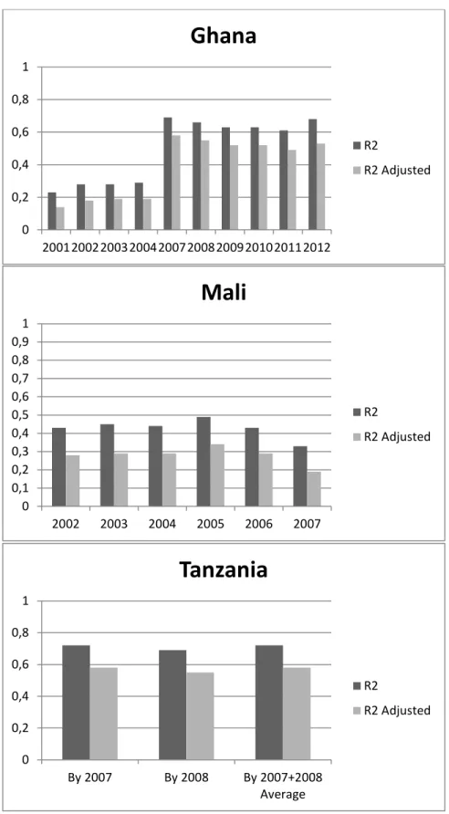
The data used to analyze the relationship between NDVI and agricultural production was obtained from the statistical offices in Ghana, Tanzania and Mali. The data was compiled on district levels and represent all agricultural products produced during one year. Ghana had data for year 2001 to 2012, Tanzania for year 2007 and 2008 and Mali 2002 to 2007.
Gross Domestic Product
Official GDP data were also obtained from the World Bank World Development Indicators open data database (The World Bank Group, 2014). Data were downloaded for each country on a yearly basis from 1992 to 2012. The official GDP data represents the value of the gross output produced in a country minus the value of intermediate goods and services consumed in production. All GDP data are expressed in constant 2005 US dollars (USD). Since the purchasing power of currency changes over time due to inflation, the use of the constant value allowed for time series comparison of the data.
3. Remote sensing and economic activities
Nightlight and economic activities
Satellite remote sensing missions are generally designed for specific applications, often earth sciences related, such as vegetation classification and weather forecasting. Very few, if any, sensors are designed for social science applications (Hall, 2010). The DMSP-OLS sensor, also known as “nighttime lights”, has attracted recent attention due to its capability to depict human settlement and development. It is sensitive enough to detect street lights and even saury fishing vessels at sea (Sei-Ichi, Fukaya, Saitoh, and Semedi, 2010). The light detected by the DMSP-OLS is largely the result of human activities, emitted from settlements, shipping fleets, gas flaring or fires from swidden agriculture. Therefore, nighttime light imagery serves as a unique view of the earth’s surface which highlights human activities. One of the central uses of the nighttime lights dataset is as a measure of and proxy for economic activity. The relationship between economic activity and light has been explored by several authors and all have concluded that there is indeed a positive relationship between the light emitted and the level of economic development within a region. This understanding has been used to estimate both GDP and economic growth.
An early identification of the strength of the relationship between nighttime lights and economic development was made by Elvidge, et al. (1997), who explored the relationship between lighted area and GDP, population and electrical power consumption in the countries of South America, the United States, Madagascar and several island nations of the Caribbean and the Indian Ocean. Using simple linear regression over a single year (1994/1995) they found that GDP exhibits a strong linear relationship with the lighted area (R2 = 0.97).
Elvidge, et al.’s (1997) publication is unique in that it deals with the relationship between economic activity and lighted area. Most other publications related to economic activity examine its relationship with light intensity. Doll, Muller and Morley (2006) were one of the first to apply this relationship to estimating economic activity on a national and sub-national basis. They identified the unique linear relationships between gross regional product (GRP) and lighting for the European Union and the United States using 1996/1997 data and found that one linear relationship was not appropriate since some cities were outliers. With these outliers removed, they were able to generate simple linear regressions for each country, with R2 values ranging from 0.85 to 0.98, and used these to generate a gridded map which estimated GRP at the five kilometer level.
Building on this research, Ghosh, et al. (2010) generated a global disaggregated map of economic activity with a spatial resolution of 30 arc seconds (approximately one square kilometer at the equator). They first performed a linear regression between gross state product (GSP), GDP and light intensity for 2006 for various administrative units in the states of China, India, Mexico and the United States to obtain an estimate of total economic activity for each administrative unit. These values were then spatially distributed within a global grid using the percent contribution of agriculture towards GDP, a population grid and the nighttime lights image. Ghosh, et al. (2010) improved on Doll, Muller and Morley (2006) through the use of the population grid and the percent contribution of agriculture as they were able to assign economic activity to agricultural areas which generate economic activity but which are not usually captured by the nighttime lights dataset since they are not often lit.
Chen and Nordhaus (2011) were one of the first to analyze the relationship between economic activity and light using a time series approach. They accomplished this by calculating the weights for light intensity that would reduce the mean squared error for the difference between the true GDP values and the estimated ones in all countries globally for 1992 to 2008. They found that light intensity has a high 8
potential to add value to GDP estimation in data-poor countries, both at the national and sub-national level. In data rich countries, light intensity data does not add as much value because its measurement error is generally higher than that of the available economic data.
One of the most recent applications of the nighttime lights dataset in relation to economic activity was by Henderson, Storeygard and Weil (2012). Rather than exploring the relationship of lights with GDP, they explored the relationship with economic growth. Like Chen and Nordhaus (2011), they performed an analysis over a time series for the period between 1992 and 2008. They developed a statistical model which estimated GDP growth using country specific economic data combined with light intensity values. Similar to Chen and Nordhaus (2011), they applied different weights for the lighting data and existing economic data based on the quality of the economic data. They found that for “bad” data countries there are often large differences (both positive and negative) between the recorded economic growth and the estimated growth. They also found that their model tended to underestimate economic growth in countries with low growth and overestimate it in countries with high growth.
All in all, the literature confirms that there is a strong relationship between nighttime lights and economic activity, both in terms of lighted area and intensity and in terms of GDP and GDP growth. Most studies have tended to be for single years, although two time-series studies were also discovered. Likewise, light intensity has been used more commonly than lighted area in analyses related to economic activity.
NDVI and agricultural production
Numerous methods exist for estimating productivity of the agricultural sector with remote sensing technology. Most approaches rely on measurements of reflected light in red and near-infrared (NIR) wavelengths where vegetation, including crops, is very reflective in the NIR and absorptive at red wavelengths. Combinations of these two wavelengths (i.e. vegetation indices) are good measures of plant vigor and are the mainstay of nearly all approaches to crop yield estimation (Lobell, 2013). Yields are then estimated through establishing the empirical relationship between ground-based yield measures and some vegetation indices, typically Normalized Difference Vegetation Index (NDVI).
Errors in remote- sensing crop- yield estimates vary mainly as a function of sensor properties (spatial-, temporal-, and spectral resolution) and landscape complexity. Classification of crop types is more problematic in regions characterized by multiple crops with similar phenologies, or in regions with intercropped fields (Lobell, 2013). Additional complexity is added with cassava, a major crop for which even farmers themselves have difficulties in estimating yields. This is basically because it is a root crop with staggered harvesting, but also widely differing above-ground architecture. Sometimes overlooked, is the problem of cloud cover in satellite based remote sensing, that could severely limit the number of available observations for a particular geographical region. Yield estimation in mixed cropping systems, characteristic of African smallholder agriculture, should nevertheless be possible, provided correct sensor platform properties.
Long-time scale analysis of NDVI can reveal important information on vegetation anomalies caused by variations in rainfall, temperature and sunlight (irradiance) as well as the trend for a certain location. Phenological metrics, such as start and end of growing season(s), length of season, time for mid of season, seasonal amplitude in NDVI, rate of increase and decrease at beginning and end of season can be related to management and crop yields for individual years as well as longer periods.
The sum of NDVI on district level is used in order to reflect the level of agricultural production. The spatial varying relationship between actual agricultural production measure as output harvested on district level and the sum of NDVI are tested through Geographical Weighted Regression (GWR).
Fig. 1. GWR Dependent variable Total agricultural production by district and Independent variable NDVI Intensity sum by district (2007)
Figure 1 illustrates the varying spatial relationship between our two estimates of agricultural production (NDVI and official statistics covering agricultural production for more estimation details see figure 3 and table 1 in Appendix). The pattern that arises is that there is a strong to medium strong relation between the variables in areas with high population densities. At this point it is difficult to access the quality of the production data in the agricultural production as large shares of production are not commercialized. We also assume that the NDVI-signal becomes more disturbed in areas of low population, less agricultural production and scattered fields.
4. Results
The result section is divided into 2 parts; Part 1 consists of a descriptive analysis of the mining buffers developed from 2 mines in each case country covering 2001 and 2012. Part 2 reports the results from the national and local growth model based on time series analysis covering the period of 2001 to 2012 at district level in the case countries. The districts have been divided into three categories; i) district with mining site, ii) district neighbouring a district with a mining site and iii) other districts.
Analysis of mining buffers
Buffers based on the distance has been created for the three remote sensing datasets to illustrate the changing patterns in terms of intensity in nightlight, forest loss and NDVI based on the distance from the mine location. For each country two mines are selected and included in the analysis.
Fig.2. The relationship between nightlight intensity and distance from the target mines
Fig.3. The relationship between forest loss and distance from the target mines
Fig.4. The relationship between NDVI intensity and distance from the target mines
Burkina Faso
Mana Mine
The Mana Mine with its satellite Siou and Fofina deposits is located approximately 200km west of Ouagadougou, the capital of Burkina Faso. The mine is operated by SEMAFO Inc, a Canadian-based
mining company. It owns 90% shares in the mine while the government of Burkina Faso holds the remaining 10%. The property covers 2,327km2 of land over the prospective Houndé belt. Gold production increased by 4.5% from 5,589kg of gold in 2010 to 5,841kg of gold in 2012. The company anticipated to increase annual production capacity of gold to about 9,300kg per year by the end of 2014 through its plant expansion program commenced at the second quarter of 2012.
Nightlight intensity shows a large increase on a radius of 10 to 30 km from the mine thereafter a decrease
in the intensity can be observed.
Forest loss for year 2001 is almost on zero levels close to the mine with increasing loss at 50 km distance
from the mine. Observations for year 2012 provides a slightly higher forest loss for locations close to the mine and lower levels of forest loss for 40 km and further away.
NDVI intensity is stable both in time and space. However, there is a major difference with a lower
intensity during 2012.
Essakane Gold Mine
The Essakane mine is located approximately 330km northeast of the country’s capital, Ouagadougou. It extends across the boundary of the Oudalan and Seno provinces in the Sahel region of Burkina Faso; situated within 42km east of the nearest large town and the provincial capital of Oudalan, Gorom-Gorom. The mine is located within a 100.02km2 mining permit area surrounded by six exploration permits covering a total of 1,383km2. From 4,230kg in 2010, production in the Essakane Mine significantly increased to 11,664kg in 2013 mostly due to a streamline of the mine’s processing plant, resulting in a 15% increase in the min’s processing rate. Though commercial production of gold began in 2010, the Essakane deposit had been an active artisanal mining site since 1985. The Office of Geology and Mining of Burkina (BUMIGEB) carried out regional mapping and geochemical programs and financed a program of heap leach test work from 1989 and 1991. From 1992 to 1999, heap leach processing of gravity rejects from artisanal mining activities were undertaken by the Compagnie d’Exploitation des Mines d’Or du Burkina (CEMOB). Upon completion of a feasibility study in September, 2007, GoldFields earned a 60% interest. Orezone Resources reclaimed ownership in October, 2007. In 2009, IAMGOLD Corporation, a Toronto-based international gold producer, acquired Orezone Resources and commenced management of the Essakane project. IAMGOLD has 90% share while the government of Burkina Faso holds 10%, non-dilutable, free-carried interest. The company targets a doubling of hard rock throughput with an expansion project that was expected to begin in 2014. The mine life has been extended to 2025 (IAMGOLD, 2012).
Nightlight intensity shows a large increase in a radius of 10km distance thereafter a sharp intensity
decrease can be observed for year 2012 which relates to the opening of the mine in year 2010. For year 2001 almost no emission of light can be observed from the buffers surrounding the location. This is explained by the opening date of the mine being year 2010.
Forest loss for year 2001 and 2012 are on zero levels for both years and at all distances.
NDVI intensity for both years follows the same trend with increased intensity from an already high level
from 10 km distance from the mine. The intensity is higher for 2012 than 2001.
Ghana
Ahafo/Subika Mine
The Ahafo Mine is located in the Brong Ahafo region of west-central Ghana, about 30km south of Sunyani and 290km northwest of the capital city of Accra. The mine is wholly owned and operated by 14
Newmont Mining Corporation, a US based gold producing company. Production started from the mine in 2006 and in 2010, 15,450kg of gold were produced. Presently, Newmont Ghana operates four open pits at Ahafo with reserves contained in thirteen pits, over a strike length of 40km. In 2011, the company continued its expansion activities in the neigbouring Subika Mine which will extend the mine life at Ahafo South.
Nightlight intensity shows low levels of nightlight up to distances of 30 km with increase of the intensity
up to 50 km from the mine. The trend is similar between the years with higher levels in year 2012.
Forest loss for year 2001 is on stable levels throughout the distance from the mine. Year 2012 follows the
same trend but with a higher forest lossl.
NDVI intensity is stable both in time and space with a slight decrease over the distance from the mine.
However, there is a major difference in a higher intensity during 2012 compared to 2001.
Chirano Mine
Kinross Mining Company acquired 90% ownership of the Chirano mine in September, 2010 after acquiring Red Back Mining Inc. The remaining 10% interest is held by the government of Ghana. Chirano is located in the southwestern part of Ghana, approximately 100km southwest of Kumasi, Ghana’s second largest city. The mine comprises 11 deposits: Akwaaba, Suraw, Akoti South, Akoti North, Akoti Extended, Paboase, Tano, Obra South, Obra, Sariehu and Mamnao. Both open pit and underground mining methods are employed. The capacity of the mill is approximately 3.5million tones per annum. In 2013, 7,807kg of gold was produced from the mine.
Nightlight intensity shows an increase on a radius of 10km to 20 km distance from the mine thereafter a
sharp decrease in the intensity both years follow the same trend.
Forest loss for year 2001 is on stable levels throughout the distance from the mine however with a small
decrease when the distance from the mine increases. 2012 follows the same trend but with forest on a higher level.
NDVI intensity is stabile both in time and space with a slight decrease over the distance from the mine.
However, there is a major difference in a higher intensity during 2012
Mali
Sadiola mine
Situated in Western Mali, the Sadiola mine lies just 77 km south of Kayes, the capital of Mali’s remote, westernmost administrative region of the same name. It is the only mine for which the government holds a stake of 18% instead of 20%, leaving 41% to Anglogold and Canadian Iamgold each. Mining at Sadiola takes place at five open-pits. The site includes a 4.9million tones per annum carbon-in-leach (CIL) gold plant where ore is eluted and smelted. New regulations introduced in the 1999 Mining Code had made the expansion of Sadiola mine possible as local population had to be resettled in the relatively densely populated Kayes region.
Nightlight intensity for year 2012 shows an increase on a radius of 10km to 20 km distance from the mine
with a stable level over 30 to 40 km away from the mine. Interesting to note is that it thereafter show a sharp decrease in the intensity and that both years follows the same trend.
Forest loss for both years is almost on zero levels on close distance to the mine with increasing loss at 60
km distance from the mine. Observations for year 2012 provide a slightly higher forest loss for locations fare from the mine.
NDVI intensity for both years follows the same trend with increased intensity from 10 km distance from
the mine. There is almost no vegetation close to the mine.
Syama mine
Syama mine is located 300 km southeast of Bamako and approximately 30km from the Côte d’Ivoire border in Sikasso region, the southernmost region of Mali.. In 2009, the surrounding Fourou Commune (1,340 km²) was home to 41,543 people, a number that had doubled in the course of one decade.
Nightlight intensity shows a large increase on a radius of 10km distance thereafter a sharp decrease in the
intensity can be observed for both years which corresponds to opening of the mine. No emission of light can be observed 40 km from the mine.
Forest loss for year 2001 is on stable levels throughout the distance from the mine. 2012 provides an
increase in 10 km to 20 km from the mine. The loss decreases thereafter to the same levels as in year 2001.
NDVI intensity for both years follows the same trend with increased intensity from 10 km distance from
the mine. There is almost no vegetation close to the mine.
Tanzania
Buzwagi mine
Located 97 km from Bulyanhulu and 6km south east of the town of Kahama in Shinyanga region, where subsistence is traditionally based around livestock and agriculture development, Buzwagi is the largest single open-pit and second largest mining operation in Tanzania. In 2011, some 2,099 workers (1,004 employee + 1,095 contractor) were employed, of which - according to ABG – 90% were Tanzanian. The mine life is supposed to end in 2022. In the three villages surrounding the mine, Mwendakulima, Chapulwa and Mwime, farming is the predominant economic activity.
Nightlight intensity shows a large increase on a radius of 10km distance thereafter a sharp decrease in the
intensity can be observed for both years however on lower levels in 2001 compared to 2012. On a distance 40 km from the mine almost no emission of light can be observed from the buffers surrounding the location up until 100 km from the mine.
Forest loss for both years is almost on zero levels on close distance to the mine with increasing loss at 50
km distance from the mine.
NDVI intensity for both years follows the same trend with increased intensity from 10 km distance from
the mine. There is limited vegetation close to the mine.
North Mara mine
North Mara mine is operated by ABG and as indicated by the name it is located in Mara region, more precisely in Tarime district 100 km east of Lake Victoria and 20 km south of the Kenyan border. The mine consists of four open-pits and, one process plant, waste rock dumps and other related facilities. As of 2012, 2,329 people were employed at the mine, of which the majority of 1,300 were contracted workers. It was opened in 2002 and is estimated to continue production until 2021. Desertification poses a major 16
challenge to the surrounding area in the region, ABG claims to combat desertification through the donation of tree seedlings to different recipients in the local communities. Furthermore, the company has stated that the power line brought to the mining site had provided local businesses and private households with stable access to electricity.
The nightlight observations from year 2001 starts on relative high levels around 10 km from the mine then decreases until 30 km and peaks to 40 km then decreases again up to 100 km from the mine. For 2012 the nightlight intensity are low close to the mine with increasing intensity up until 40 km thereafter decreases. Forest loss for both years is almost on zero levels on close distance to the mine with increasing loss at 50 km distance from the mine. Whereas observations from year 2011 reach an increase in forest loss at 40 km and with sharp decrease in forest loss from 40 to 50km. 2012 indicate a steady increase of forest loss from 20 and further away from the mine.
NDVI intensity for both years follows the same trend with increased intensity from 10 km distance from
the mine. There is almost no vegetation close to the mine which confirms the descriptive information from the mine highlighting the problem of desertification around the mine.
National growth model
Our basic estimation strategy follows what Henderson et al. (2012) developed. Their framework can be shown as equation (1):
(1) γjt = ψ�xjt+ cj+ dt+ ejt
where …𝛾𝛾𝑗𝑗𝑗𝑗 is the true GDP of country j in time t. 𝑥𝑥𝑗𝑗𝑗𝑗 is the level of observed nighttime light at corresponding country and time. 𝑐𝑐𝑗𝑗, 𝑑𝑑𝑗𝑗, and 𝑒𝑒𝑗𝑗𝑗𝑗 stands for country effect, year effect, and error term. The assumption for this model is then that, no matter the type of economic activities on the ground, their aggregated growth results in the same percentage growth of nighttime light observed by satellite plus, country-invariant, time-invariant effects and an error term. The basic regression analysis assumption requires that the error term be a random variable with a mean of zero. However, we have shown through gridded data of land cover and nighttime light that it is possible for agriculture’s value-added to increase without emitting more observable nighttime light into space. If this is the case, then the error term is actually dependent on the agricultural share as the higher the agricultural share the higher the error terms. Randomness of the error term from independent variables is one of the important assumptions of regression analysis. It is therefore desirable to exclude activities that can grow without emitting more nighttime light.
This paper makes full use of the statistical framework in equation (1) and estimation strategy proposed by Henderson et al. (2012). However, we have revised the assumption that all economic growth is captured by growth in observed nighttime light. Our revised assumption is that nighttime light observed in space is the result of growth in only the non-agricultural sector. We therefore divided Henderson et al. (2012) into non-agricultural (eq. 2) and agricultural (eq. 3) parts with a combined model as illustrated in (eq. 4). Based on our discussion in previous sections, previously we introduced MODIS land cover product MCD12Q1 (Keola et al. 2014).
(2) γjtna = ψ�naxnajt + cjna+ dtna+ ejtna (3) γjta = (ψ�a1 ψ�a2 … ψ�an) ⎝ ⎜ ⎛ljt a1 ljta2 ⋮ ljtan⎠ ⎟ ⎞ + cja+ d t a+ e jt a
In this paper our extended model is refined by changing the categorical variable land cover to estimate agricultural development with using MODIS NDVI and forest cover. A national growth model has for each country been developed using nightlight, NDVI, and forest loss. The models are based on a multiple linear regression between the three variables and national GDP, as can be seen in equation 4.
The presented models are developed without allowing for an error (interception) term which is due to an initial analysis that showed that the downscaling, from national growth to district growth, was highly influenced by the error (interception) term hence reducing the model applicability at district scales. The resulting models are for each country presented and analyzed in the sections below
Fig. 5. Model results for growth patterns (2001-2012) in case countries. (4) GDP ~ Nightlight + Forestloss + NDVI
Burkina Faso
For Burkina Faso the resulting national model showed a similar trend as real GDP (figure 5a) but had some inconsistency between years indicating that the model does not manage to completely capture the country level GDP. The model had a residual standard error of 8.33E+11 which is about 30% of the average national GDP. Furthermore, the model had significant coefficients for nightlight and forest loss which indicates that those two are the best predicting variables for Burkina Faso (table 2).
Ghana
For Ghana the resulting national model showed a good agreement with real GDP (figure 5b). It captured the constant state for the first years and increased from around year 2007. The model had a residual standard error of 1.39E+10 which is about 52% of the average national GDP. Furthermore, the model had significant coefficients for nightlight and NDVI which indicates that those two are the best predicting variables for Ghana (table 2).
Mali
For Mali the resulting national model showed a good agreement with real GDP (figure 5c) by showing approximately the same increase and values as real GDP. The model had a residual standard error of 1.29E+12 which is about 9% of the average national GDP. Furthermore, the model had significant coefficients for nightlight and NDVI which indicates that those two are the best predicting variables for Mali (table 2).
Tanzania
For Tanzania the resulting national model showed a good agreement with real GDP (figure 5d) up until year 2008 and after that showing some inconsistent results. The model had a residual standard error of 9.28E+12 which is about 42% of the average national GDP. Furthermore, the model had a weak significant coefficient for forest loss which indicates that it is not the best predicting variable for Mali (table 2).
Table 2
Multiple linear regression coefficients for growth model specified in equation 1. Burkina Faso Ghana Mali Tanzania Nightlight 2.75E+07 *** 3.60E+05 *** 2.46E+06 ** 5.98E+07 Forestloss 2.81E+07 * 3.56E+04 4.83E+05 1.30E+07 . NDVI -8.77E-02 -5.01E+01 ** 1.29E+12 *** -3.68E+03 Signif. codes: ‘***’ 0.001 ‘**’ 0.01 ‘*’ 0.05 ‘.’ 0.1 ‘ ’ 1
We note that the growth model in some cases produce negative coefficients for NDVI (Table 2). This is caused by varying agricultural production systems and a complicated vegetation mosaic, typical for these regions. We note, for example, that agricultural intensification or expansion not necessarily generates electrification. We know thou that increase in production often relies on expansion which means clearing of non-agricultural areas, often in forest or semi-forested areas. Low values of NDVI are related to less vegetation, for example, bare soil after clearance, conversion of grasslands to urban fabric, etc. Most probably will the new crop not fully compensate for the loss of biomass by deforestation, unless manure and irrigation systems are utilized which is rare in small holder agricultural systems.
Table 3
Standard error of residuals between model and observed together with average of observed and modeled GDP.
Burkina Faso Ghana Mali Tanzania
Average GDP 2.83E+12 2.67E+10 1.44E+12 2.23E+13 Average model GDP 2.64E+12 2.68E+10 1.44E+12 2.21E+13 Residual standard error 8.33E+11 1.39E+10 1.36E+11 9.28E+12
Growth model on district levels
The results from the national growth models for each country are used to determine individual country models to estimate growth on district levels. The models are based on the regression results presented in Table 1. When developing the growth model for districts several methods where used into order to provide an accurate local dimension of the local economy. Population data, and average household expenditure on district levels were included as weights in the model estimating local growth patterns. However, population on district level was highly correlated with nightlight intensity on district levels and average household expenditure was highly correlated with GDP (for details on the correlation analysis see Appendix) and therefore removed from the estimations.
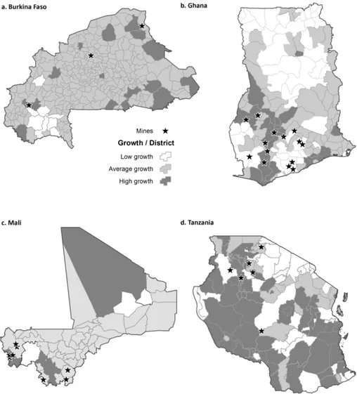
The analysis of the results from the district growth model are divided into five parts; i) a spatial analysis of the growth model reported in thematic maps dividing the districts into positive, negative or no growth districts in order to highlight the geographical patterns of district growth in each country, ii) a spatial analysis of the growth constructed by the agricultural sector reported in thematic maps dividing the districts into low and high growth districts in order to highlight the geographical patterns of district growth in each country, iii) a spatial analysis of the growth constructed by the non-agricultural sector reported in thematic maps dividing the districts into low and high growth districts in order to highlight the geographical patterns of district growth in each country, iv.) graphs illustrating the average growth based a on categorization of the districts analyzed in order to compare districts with a mine (category I), with districts neighboring a mine (category II) and with districts with no mines (category III), v.) graphs illustrating all districts average growth levels.
Fig. 6. Spatial analysis of average growth in districts (2001-2012) estimated by growth model.
Fig. 7. Average district growth separated in categories (2001-2012).
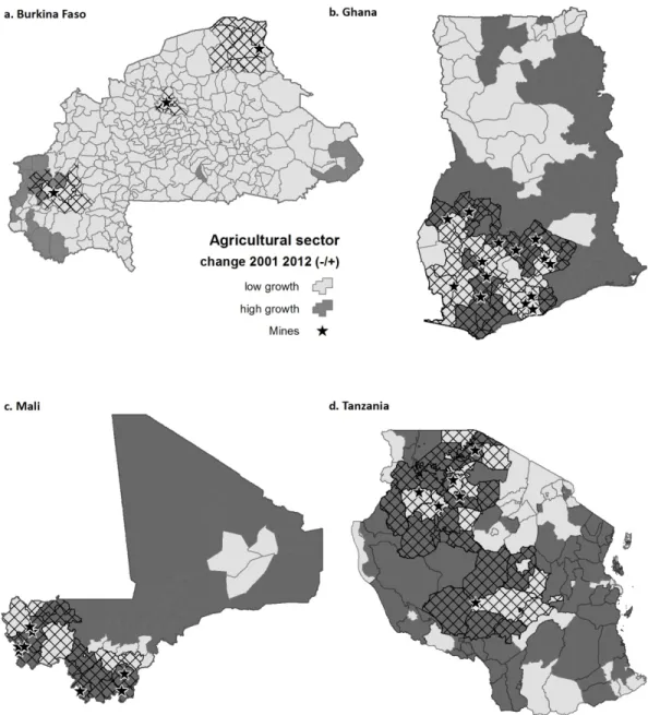
Fig. 8. Spatial analysis of agricultural growth in districts (2001-2012) estimated by growth model.
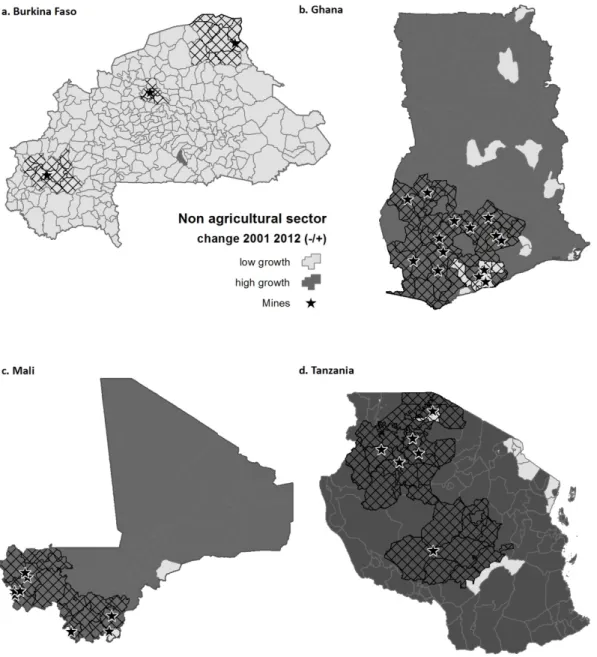
Fig. 9. Spatial analysis of non-agricultural growth in districts (2001-2012) estimated by growth model.
Burkina Faso
Burkina Faso shows spatially fragmented growth on district levels with large parts of the country indicating average growth as seen in Figure 6a. However, the northeastern part of the country high growth patterns can be identified possible through the large size of the districts in that area of the country. The southern parts of the country account for lower levels of growth. The effects of having a mine located in the district are evident in the case of Burkina Faso as seen in (Category I, Figure 7a). The country as a whole account for low levels of growth where the three districts with mines we are analyzing account for considerable higher growth. The possible causal link between mining location and growth can be problematic in this case as we only base our conclusions on three mines. Figure 10a highlights Bobo-Dioulasso the country´s second largest city with an expanding mining industry as the district with the
highest levels of growth in the country. Interesting to note is that the district with lowest levels of growth is located on close distance to Bobo-Dioulasso namely Siderdougou. When analyzing the different patterns in terms which sector driving the growth in the country Figure 9a indicates very low contribution of the non-agricultural sector from the growth model. On the other hand there patterns of high growth within the agricultural sector especially in the western parts of the country as shown in Figure 8a. Overall the division between the sectors provides support to the analysis illustrated in Figure 6a – growth is driven by a few districts.
Ghana
The patterns of growth in Ghana shows a spatial distribution to the southern parts of the country where high growth districts are located on the coastline. The northern parts of the country provide lower levels of growth as shown in Figure 6b. When the growth model is divided into the two sectors we can see that the agricultural growth as illustrated in Figure 8b follows the patterns of Figure 6a. Here is important to highlight high growth in districts neighboring a district with a spatial analysis of the growth constructed by the agricultural sector reported in thematic maps dividing the districts into low and high growth districts in order to highlight the geographical patterns of district growth in each country mine for both the agricultural sector and the non-agricultural sector (Figure 9b). However, Ghana is the only studied country where districts with a mine is associated with negative growth patterns as indicated in Category I, Figure 7b. However, the country as a whole indicates stable positive growth. The areas with highest growth figures are found in Figure 10b which indicates the capital Accra and a district with a mine named Atwima. Overall growth patterns distributed on district levels show positive level with a few as indicated in Category I, Figure 7b.
Fig. 10. Average district growth in each country (2001-2012).
Mali
Mali shows a high growth both in the northern and southern part of the country, as seen in Figure 6c. In the southern part this is proposed to be due to a combination of the urban area of Bamako and the location of the mines. However, in the northern part the higher growth is mainly due to a spatial size dependency of the model which most likely generated a falsely estimated high growth. This since the area mostly consists of desert. However, it is also influenced by the urban areas in the southern part of the district close to river Niger. When analyzing the agricultural sector´s contribution the growth we can identify that large parts of the country experience high growth as shown in Figure 8c.For the non-agricultural sector almost all districts experience high growth (Figure 9c). It can be seen that districts with a mine (Category 26
I, Figure 7c) shows a higher growth than average and that districts neighboring to a mine (Category II) shows a lower than average growth. It can be seen, overall, that almost all the districts in Mali shows a positive trend in the economic growth (Figure 10c). The high growth in the northernmost district Timbuktu, shown in Figure 10c, is again proposed to be due to model errors and the urban areas in the southern part of the district.
Tanzania
Tanzania shows spatially fragmented growth between the districts, as can be observed in Figure 6d. Most of the mines are, however, located in or close to districts with high growth. However, when analyzing the growth patterns within the agricultural sector we can see that the districts with a mine are all experiencing high growth (Figure 8d). The patterns within the agricultural sector is scattered between the districts. This finding is further supported with that Category I and II shows a slightly higher growth than the average (whole), as can be seen in Figure 7d (Category I + II). Interesting to note is that districts neighboring to a mine (Category II) shows on average a higher growth than districts with a mine (Category I). The non-agricultural sector provides high growth in almost all districts – with a few exceptions as illustrated in Figure 9d. The district growth model was able to correctly identify the urban region Lushoto as a district with high growth (Figure 10d). However, Bukombe which is a mining district was identified as a district with negative growth (Figure 10d) which was an unexpected result. However this could be due to the location of the mine which is on the border to a high growth region (Figure 6d, westernmost mine).
5. Night Lights, NDVI and Forest Coverage in a
Difference-in-Difference Framework
5Empirical Framework
To understand if night lights, greenness and forest coverage change in mining communities with mining onset, we employ an empirical estimation strategy called difference-in-difference (previously employed to understand the economic effects of gold mining in Africa by Aragón and Rud (2013), Tolonen (2015), and Kotsadam et al., (2015). This strategy allows us to compare outcomes in the geographic proximity of mines, with areas further away, both before and after the mines start producing. In effect, we are making three comparisons: close-far away, as well as before-after, and both comparisons at the same time. We can model the cross-sectional differences in areas with an active mine, and without active mines:
Yjt = β1activejt+ εj
Where Y is the outcome variable (night lights, NDVI and forest cover), active is a binary variable that takes value 1 if the mine is active in that year, and subscript j is for the mine, and t for the year. We can also model the importance of proximity:
Yj= β1closej+ εj
Where close captures the cross-sectional difference between areas that are close to mines and those that are further away. What we are interested in knowing, however, is the relative change that happens with mine onset in the geographic proximity of mines, compared to far away. We capture this with the difference-in-difference estimation model which includes an interaction effect of the two binary variables:
Yjt = β1activejt+ β2closej+ β3activejt∗ closej+ δj+ εjt
Where δj is a mine fixed effect, which means that we only look at changes within a mine. We can also use year fixed effects, which will take care of year-specific shocks that happens across all mines. To decide the relevant distances, we rely on Aragón and Rud (2013), Tolonen (2015), and Kotsadam et al., (2015), who show that areas at up to 20km radius are relevant to use to understand the footprint of gold mines in Africa. Moreover, we rely on the geographic results found in this paper. We chose a distance of 20km to understand the footprint close to mines (10km is not possible because of lack of quality spatial data at this resolution). We compare with an area which is 50 to 100km away, drawing from the same literature--- it has been shown that beyond 50km, the mines have little economic footprint and, is thus suitable as a comparison group.
5 The econometric analysis was conducted by Anja Tolonen.
28
Results
Graph 1 explores the change in the two groups, close and far away, over the mines’ lifetime. On the horizontal axis is the mine year, counting from 4 years before mine opening, highlighted by the red vertical line, to four years after mine opening. The graphs are based on summary statistics, and we do not control for any systematic differences across the mines included here. Overall, it seems like areas very close to mines are on a steeper trend in night lights than are areas further away, especially as we get closer to the mine opening year which is highlighted by the red vertical line. One interpretation of this pattern is that from a few years before the mine starts extracting gold, economic activity increases in these areas. A reason why this happens before the actual mine opening year is because mines are capital intensive and the local economy is stimulated during this investment phase, a pattern confirmed in previously mentioned econometric studies.
For NDVI we do not see a big difference across the areas, although both areas seem to be on an upward sloping trend--- although this needs to be interpreted with caution, because it can be driven by the unbalanced sample. We cannot see a clear pattern for forest coverage, but areas close to the mines have higher forest coverage in general. This is highlighting that mines open in more rural areas that in general have higher levels of forest coverage.
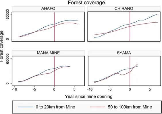
Graph 2, 3, and 4, show the same summary statistics but for each individual mine. For night lights, there is a divergence for most mines in the sample as we get close to the mine opening year, and a convergence after a few years in some of the cases (Ahafo, Chirano and North Mara). We have less data points for NDVI and we discern almost no changes across the areas, neither is there a clear pattern for forest coverage (Graph 4). If anything, we detect that close mining areas are getting relatively greener over time, compared with further away. Graph 1: Night Light, NDVI and Forest Coverage over Mine Lifetime Graph 1
Night Light, NDVI and Forest Coverage over Mine Lifetime
Graph 2
Night Light by Mine
Graph 3 NDVI by Mine
Graph 4
Forest Coverage by Mine
Table 4 shows the mean values in areas close to mines and far away from mines, but not taking into account the time-variation in mining activities. Mining areas have higher night light score, and are greener on average, compared with 50 to 100km further away.
Table 4
Mean values in Night lights, NDVI and Forest Coverage
0 – 20 km 50 – 100km Observations
Night Lights 7276.43 2899.59 134
NDVI 95387.83 63633.97 60
Forest Coverage 33463.83 28132.51 48
Notes: Summary statistics (mean) value for the three outcome variables across the treatment and control
group, in the cross-section.
Table 5 shows the regression results from the strategies outlined in the Empirical Framework section. Active mine areas have higher level of lights at night (Column 1, Panel A), and close areas do too (Column 2, although insignificant). The interaction effects (Columns 3 and Column 4, Panel A) are both insignificant, meaning that we do not see a significant difference in night lights close to active mines---
although the effect is positive6. This is suggestive evidence that gold mining spurs local economic growth, and is in line with evidence showing that gold mining can bring local structural change by generating non-farm employment (Kotsadam et al., 2015; Tolonen, 2015).
Table 5
Cross-sectional and time variation in Night lights, NDVI and Forest Coverage
(1) (2) (3) (4)
VARIABLES Active Close Interaction Interaction
Panel A: Night Lights
Active*Close 1,501.879 1,541.769 (2,278.851) (2,372.862) Active 2,706.309* 1,865.767*** 26.513 (1,124.946) (396.321) (1,131.337) Close (20km) 4,104.690 3,621.344 3,603.291 (3,444.181) (3,082.794) (3,208.017) Panel B: NDVI Active*Close 3,979.000 4,444.185 (2,697.911) (2,630.807) Active 1,924.360 -292.512 -1,172.214 (1,597.637) (1,942.894) (2,014.870) Close (20km) 22,519.634*** 20,530.133** 20,297.541** (4,790.365) (5,169.214) (5,338.961)
Panel C: Forest Coverage
Active*Close 5,735.336 5,735.336 (13,328.923) (14,237.795) Active 12,361.557* 9,493.889 15,184.385** (4,891.403) (5,618.271) (3,559.078) Close (20km) 5,331.320 2,583.138 2,583.138 (13,221.950) (8,368.023) (8,938.622)
Mine fixed effects Yes Yes Yes Yes
Year fixed effects No No No Yes
Notes: Active is a dummy variable which takes a value of 1 if the mine was actively producing in year t, otherwise 0.
Close takes a value of 1 if within 20km from a mine, otherwise 50-100km. Active*Close is an interaction term, capturing the effect of being close to an active mine. Observations in Panel A, N=281, in Panel B, N=132 and in Panel C, N=96. Close is defined as within 20km from the mine site (center point), and far away is 50 to 100km away. Panel A include mines Ahafo, Buzwagi, Chirano, Essakane, Mana, North Mara and Syama. Panel B include Ahafo, Chirano, Essakane, Mana, Sadiola and Syama and Panel C include Ahafo, Chirano, Mana and Syama. Clustered standard errors at the mine level in parentheses. *** p<0.01, ** p<0.05, * p<0.1.
6 According to the visual evidence presented in Graph 1, where the local economy is spurred roughly 2 years before
mine opening, we drop the years immediately preceding the mine opening from the regression in a robustness check. The results are slightly larger for the interaction term, as expected, but remain insignificant. The results from this exercise are available upon demand.
32
Note however, that if households engaging in subsistence farming do not have, and need, electricity access change to more modern sectors which demand electricity at mine opening, this will cause an increase in night lights. In such a scenario, we may overestimate the effect of the mine on the local economy since the decrease in farming is not associated with any change in night lights, if it was not reliant on electricity for power. However, Kotsadam et al., (2015) estimate that non-migrant households that live close to gold mines in Ghana have better access to electricity, which is in line with this finding.
If mines increase the urbanization rate or lead to decreased local farming (as found by Aragón and Rud, 2013), greenness in mining areas should decrease. We have to measures of greenness; NDVI as well as forest coverage (which captures permanent greenness, rather than the seasonal variation in greenness stemming from farming activities). Panel B shows that close areas have higher levels of NDVI (Column 2, 3, and 4): this is indicative of mining areas being more rural in general. However, the interaction terms (Column 3 and 4) are positive indicating that NDVI increases with the onset of mining. We do not have any theoretical predictions supporting this finding, but note that the estimated effect is insignificant and very small relative the already higher level of greenness close to mines (coefficient for close). The analysis thus points toward no significant change in NDVI. Similarly, we do not estimate a significantly different level of forest coverage (Panel C) with the mining activities. One caveat here is that the sample sizes are quite small since we are only looking at a handful of mines. This might thus limit the possibilities to precisely estimate the effects of mining on NDVI and forest coverage. Moreover, the mines selected in this analysis vary across the three measures and remains a selected sample of the gold mines in the region.
6. Conclusions
The objective of this study was to use remote sensing data to estimate level and growth (or decline) of economic activities in reference to the mining industry in Burkina Faso, Ghana, Mali and Tanzania by comparing estimated levels and changes in agricultural and non-agricultural production in mining and non-mining localities. Our study identified 32 mines within the studied countries as prime study areas. The analysis was divided in to 2 parts. Firstly, 8 mines (2 per country) were chosen and studied using spatial analysis using three types for remotely sensed data namely nightlight intensity, NDVI intensity and forest loss intensity based on the distance. Secondly, the paper estimated growth in economic activities on district levels in the studied countries to compare economic growth patterns in districts with a mine, districts neighboring a district with a mine and other districts that are not close to a mine. The remote sensing data sets used in the study covered a period from 2001-2012 providing not only high spatial resolution but also a time series perspective in order to account for change over time and a validation vegetation index from satellite images with agricultural production statistics from the ground.
The data used in the study has after processing been assembled into a geodatabase with the working title “African Economic Growth, light and vegetation database” (AEG, 2014).
Results from the first section provide detailed information about the relationship between distance to a mine and the intensification of vegetation, forest loss and nightlight. Among the studied 8 mines we can observe individual patterns where the mines located in Mali and Tanzania are located in areas with almost no vegetation with an increasing intensification with the increased distance from the mine. The trends are identical from 2001 and 2012. However, for Ghana and Burkina Faso our result indicates that the studied mines are located in areas with high intensity of vegetation. Particularly, Ahafo and Chirano provide interesting results in terms of increasing levels of vegetation from year 2001 to 2012. The levels of intensification are stable with the distance from the mine.
A clear pattern in terms of nightlight is that the intensification increases during the years associated with an establishment of a mine. This confirms knowledge from the ground saying that activities omitting nightlight are common during the establishment of a mine. Results from the second part of the analysis focusing on modelling growth on districts levels in each of the studied countries using remote sensing data to account for non-agricultural activities (nightlight) and agricultural actives (NDVI and forest loss). The objective is this part is to compare districts with a mine and districts neighboring a district with a mine with districts without a mine. Our results show that districts with a mine account for higher growth than districts without a mine – this result holds for Burkina Faso, Mali and Tanzania. Ghana provides results in opposite direction giving lower growth for districts with mines.
Despite the popular view of large-scale mines as economic enclaves separated from the local economies, this analysis of a selected set of gold mines from four African countries (Burkina Faso, Ghana, Mali and Tanzania), shows that economic activity as proxied by night lights, increase in the mines’ close proximity. Proximity is defined to an area within 20km from mine center point, and the control group is drawn from an area 50 to 100km away. However, this estimate remains statistically insignificant and we urge future analyses to further assess the causality of this pattern using a larger and more representative set of mines. Despite the risks that mines can decrease agricultural productivity, through e.g., environmental pollution or structural shifts on the labor market, we do not find a decrease in greenness. Moreover, forest coverage does not seem to change significantly with large-scale mining. One caveat to this analysis is the strongly selected, handful set of mines that are analyzed, and that they only represent large-scale mines. The effects of small-scale and artisanal mining activities, common in the study countries, upon economic growth and greenness are thus not discussed within this report.