Estimating interaction delay in bicycle traffic from point
measurements
Fredrik Johansson (VTI) CTS Working Paper 2018:18 Abstract
Planning for bicycle traffic is getting increasingly popular in cities, often motivated by that it is beneficial for the environment and the public health, and that it is a space efficient mode of transport. However, research on bicycle traffic has traditionally focused mainly on safety and mode choice, and less on traffic engineering topics such as investigating travel times, delays, and capacities. This study contributes to filling this gap by presenting a general method to estimate a volume -- delay function for bicycle traffic based on point measurements of passage time, speed, and lateral position, and, using estimates of the value of time in bicycle traffic, estimating the marginal cost of the interaction delay.
The proposed method is based on an established method to estimate the distribution of desired speeds, and extends this to estimate the delay of the observed cyclists. The method is demonstrated using a data set from a bridge in Stockholm, Sweden, showing that there is significant interaction delay and associated cost even for relatively modest volumes, implying that interaction delay and its cost should be considered when planning for bicycle traffic.
Keywords: Bicycle traffic, Marginal cost, Delay
Centre for Transport Studies SE-100 44 Stockholm
Sweden
Estimating interaction delay in bicycle traffic from
point measurements
Working paper Fredrik Johansson*
VTI, Swedish National Road and Transport Research Institute, Box 8072, 402 78 Gothenburg
October 8, 2018
Abstract
Planning for bicycle traffic is getting increasingly popular in cities, often motivated by that it is beneficial for the environment and the public health, and that it is a space efficient mode of transport. However, research on bicy-cle traffic has traditionally focused mainly on safety and mode choice, and less on traffic engineering topics such as investigating travel times, delays, and capacities. This study contribute to filling this gap by presenting a gen-eral method to estimate a volume – delay function for bicycle traffic based on point measurements of passage time, speed, and lateral position, and, us-ing estimates of the value of time in bicycle traffic, estimatus-ing the marginal cost of the interaction delay.
The proposed method is based on an established method to estimate the distribution of desired speeds, and extends this to estimate the delay of the observed cyclists. The method is demonstrated using a data set from a bridge in Stockholm, Sweden, showing that there is significant interaction delay and associated cost even for relatively modest volumes, implying that inter-action delay and its cost should be considered when planning for bicycle traffic.
1 Introduction
Planning for bicycle traffic is getting increasingly popular in cities, often moti-vated by that it is beneficial for the environment and the public health, and that
it is a space efficient mode of transport, making it obvious that it should be pri-oritized to get more people to bike. However, as Börjesson and Eliasson (2012a) argues, also the benefit for the existing cyclists should be included in the valuation of any improvement of traffic conditions.
One important cost of bicycle traffic, as well as all other forms of traffic, is the cost of the travel time, and thus the cost of interaction delay. This has since long been recognized in studies of motorized traffic, where efforts have been made to investigate this marginal cost of introducing one additional vehicle into the traffic stream, see e.g. Nilsson and Haraldsson (2016).
Hoogendoorn (2005) proposed a method to estimate the distribution of free speeds in motorway traffic from point measurements of speed, headway, and lane. The method, based on composite headway modeling by Buckley (1968) and the method of censored observations by Kaplan and Meier (1958), estimates a distri-bution of desired speeds and also, for each observed vehicle, estimates the prob-ability that it is constrained by the preceding vehicle. Hoogendoorn (2005) also demonstrated the method using motorway traffic data, and validated it using mi-croscopic simulation. The method was recently adopted to handle bicycle traffic by Hoogendoorn and Daamen (2016), who also demonstrated it using data from bicycle traffic in the Netherlands.
In this paper we propose a method to, based on the output of the method by Hoogendoorn and Daamen (2016), estimate the delay experienced by the observed cyclists, and from this estimate a volume – delay function. By combining this with an estimate of the value of time we also estimate the marginal cost of the interaction delay. The method is demonstrated using data collected on a bridge in Stockholm, Sweden, using a system based on video analysis provided by Viscando Traffic Systems.
The delay, and the corresponding cost, estimated by the method, is the inter-action delay on a link, not close to an intersection. This is the delay caused by the congestion on the link, not including any delay caused by anything else, such as traffic control, geometry and quality of the road. The main cause of the interac-tion delay is the heterogeneity in the desired speed over the populainterac-tion of cyclists in combination with limited overtaking opportunities, that is, slower cyclists gets in the way of faster ones, who are forced to slow down if they cannot overtake. Since the heterogeneity of the desired speed is larger for bicycle traffic than for car traffic in most situations, the interaction delay is expected to be larger for bicycle traffic, given similar traffic conditions and overtaking possibilities.
It is important to emphasize that the interaction delay on links is likely to constitute only a part of the delay experienced by typical cyclist during a typical trip. In an urban setting with many signal-controlled intersections, the delay in-duced by the traffic signals is likely to outweigh the interaction delay estimated in this paper. Traffic signals also cause interaction delay through the formation
of platoons, that, depending on the overtaking possibilities, can take significant time to disperse. Neither this delay is included in the estimation presented in this paper, even though it is interaction delay on a link. An important assumption in the method is that the platoon formation and dispersion is in equilibrium, which only is the case if there is no traffic signal too close upstream, or any change in overtaking possibilities, for example due to a change in the width of the bicycle path. If the infrastructure is not taken as a given, also the geometric delay can be significant for bicycle traffic. This is the delay induced by the shape of the bicycle path, e.g. sharp curves that forces the cyclists to slow down.
It is also important to note that non-zero delay is impossible to observe di-rectly. The delay is the difference between the actual observed speed and the desired speed. Since we, in most cases, cannot with certainty determine if a cy-clist is following the cycy-clist ahead, that is, if it is constrained by it, we do not know if a cyclist is traveling at their desired speed or a lower speed. And even if we could determine that a cyclist is following, we do not know their desired speed, so the delay is not directly observable. The approach in this paper is to estimate the expected delay based on an estimate of the probability that a cyclist with a given headway is following, and an estimate of the distribution of desired speeds.
The method does not include delay directly caused by road users other than the cyclists in the studied direction. For example, delay caused directly by pedes-trians, or cyclist traveling in the opposite direction, intruding on the bike lane forcing a cyclist to slow down is not captured. Since only cyclists traveling in one direction is considered, the perturbed cyclist will be assumed to have the ob-served speed as their desired speed, since there are no cyclists in front (that are traveling in the same direction). This will cause an underestimation of the delay, since it will include slow, in reality constrained speeds, into the desired speed distribution. However, delay caused indirectly by such events is captured, that is, the delay of all cyclists that are forced to slow down due to cyclists who are forced to slow down due to road users not included in the analysis, is included.
The method is presented in section 2, starting with a summary of the method by Hoogendoorn and Daamen (2016), followed by the proposed extension to esti-mate the interaction delay. Then in section 3 the method is demonstrated on data from a bridge in Stockholm, starting with a description of the site and an overview of the available data, and concluding with the results of the case study. Finally, in section 4 and section 5 some conclusions are drawn and some discussion on the applicability of the method and possible further research is provided.
2 Method
We here propose an extension of the method proposed by Hoogendoorn and Daa-men (2016), to additionally estimate the delay of the observed cyclists. This allows us to estimate a volume – delay relationship for bicycle traffic and to estimate the marginal cost of interaction delay.
The method by Hoogendoorn and Daamen (2016) provides us with estimates of the distribution of the desired speed and the probability that a cyclist is con-strained, that is, is following another cyclist, as a function of their headway (head-way denotes, throughout this paper, the time between passages of cyclist, that is, the time front to front). Using these two pieces of information we propose a method to estimate the delay of the observed cyclists and thereby a volume – delay relationship. This volume delay relationship is then used to estimate the marginal cost of the interaction delay. All estimations of distributions are parameter free, that is, we do not assume a specific functional form of the distributions.
2.1 Estimating the distribution of desired speeds
Hoogendoorn and Daamen (2016) estimate a composite headway model in line with Buckley (1968), assuming that cyclists are generated with exponentially dis-tributed headway and that the preferred following headways can be modeled as i.i.d stochastic variables. Furthermore, it is assumed that a cyclist never keep a smaller headway to the preceding bicycle than their preferred following headway, and that an observed headway is a realization of a stochastic variable that either follow the distribution of free headways or the distribution of preferred following headways.
The distribution of preferred following headways is assumed to vanish for headways larger than a certain threshold, which implies that the arrival rate of the free vehicles can be estimated directly from the observations of headways larger than this threshold. The threshold itself can be found by identifying below which headway the total headway distribution starts deviating from an exponential dis-tribution. This can be achieved by plotting the survival function on a logarithmic scale and identify where it deviates from a line. This deviation is, however, grad-ual, so an exact threshold is not possible to identify, thus, sensitivity analysis with respect to the threshold is recommended.
A complicating factor of bicycle traffic compared to car traffic is that bicycles do not strictly drive in separate lanes. Thus, it is necessary to make a somewhat arbitrary distinction of when a cyclist is affected in its longitudinal behavior by the preceding bicycle and when it has enough lateral separation to be considered to be independent of it, similar to a car in another lane. Hoogendoorn and Daamen (2016) take a pragmatic approach to this problem and assume that the cyclist is free if the lateral separation is large enough for it to pass by without collision,
that is the lateral separation, measured center to center, should be larger than the width of the handlebars, which usually is the widest part of a bike, plus a small safety margin.
The assumptions lead to an integral equation relating the free, following, and total headway distributions. Intuitively the equation states that the free head-ways are exponentially distributed for large headhead-ways, but for headhead-ways below the above-mentioned threshold the distribution is scaled down with the probabil-ity that a cyclist has a preferred following headway smaller than the present head-way. That is, it encodes that a free headway cannot be smaller than the preferred following headway of a cyclist. This integral equation can be solved iteratively by making the initial ansatz that the free headway distribution is the exponential distribution that best fit the headway data for headways larger than the threshold.
The quotient between the preferred following headway and the total headway probability density functions gives the probability that an observation of a head-way of a certain length is a preferred following headhead-way, that is, that a cyclist with a headway of the given size is constrained. These probabilities are then used in a version of the method of censored observations by Kaplan and Meier (1958) to es-timate the distribution of desired speeds. The application of the Kaplan and Meier (1958) method to desired speed estimation was proposed by Hoogendoorn (2005), who also extended the method to consider partially censored data. The method regards the speed observations as censored observations of the desired speed dis-tribution and take advantage of the information in an observation of a following cyclist that its desired speed is at least the observed speed. This is achieved by constructing the estimate of the survival function of the desired speed from the product of a sequence of conditional probabilities of higher desired speeds.
The original method by Kaplan and Meier (1958) requires that the observations are categorized into censored and not censored observations, that is, into free or following cyclists, but Hoogendoorn (2005) extend the method to also handle a probabilistic categorization, like the one given by the composite headway model. This is achieved by duplicating the data N times and categorize a fraction, equal to the probability of following, of the copies of a real observation as censored and then applying the original method in the limit when N → ∞.
An important feature of the method briefly described above is that it com-pletely avoids explicit consideration of how the lack of desire and possibility of overtaking contribute to the build-up of platoons, even though the existence of platoons is what causes interaction delay. This is possible due to the assumption of exponential distribution of free headways above the maximum size of follow-ing headways. This assumption enables the treatment of the result of the limited overtaking possibilities, the existence of platoons, without explicit consideration of the choice to overtake or not, but rather directly from the headway statistics.
enters the analysis, and that is when we determine which cyclist that is to be treated as the one directly in front. As mentioned above, a cyclist is not considered following the cyclist ahead if its lateral separation is a little bit more than the width of a handlebar. Of course, cyclists may have large lateral separation to the cyclist ahead but still consider themselves to be following it, rather than being independent of it. However, to not overestimate the delay all such cyclists are interpreted as independent of the one ahead.
2.2 Modification desired speed estimation method
The method proposed by Hoogendoorn and Daamen (2016) assumes bicycle traffic similar to car traffic at a multi-lane motorway, with all lateral positions more or less equivalent. However, many Swedish cycling paths, and the one under investigation in the case study of this paper in particular, are more similar to rural roads with one lane in each direction. The cyclists stay more or less in one ’lane’ during most of the time, except for short periods of overtaking, during which the cyclists temporarily change their lateral position, and then return to the main ’lane’ when the overtaking is completed.
In the case of interest to Hoogendoorn and Daamen (2016), with cyclists more or less evenly distributed over several lanes, all headways in all lanes could be treated in the same way and included in the total headway distribution. In the case of interest here, on the other hand, headways increase rapidly with the lateral displacement of the cyclist from the main stream, introducing large headways that would be highly unlikely if the traffic was evenly distributed over the lateral position. Thus, if the method by Hoogendoorn and Daamen (2016) was to be applied naively to the case of interest here, the headway distribution would be biased toward large headways as compared to an exponential distribution due to overtakings.
To adapt the method of Hoogendoorn and Daamen (2016) to the case of inter-est here, we propose to exclude from the analysis all cyclists that are not in the main stream. More precisely, considering cyclists traveling in a specific direction, we exclude any cyclist that has a lateral displacement from the median lateral position of more than 0.5 m. The cyclists that are excluded in this way from the headways modeling are all assumed to be free, and thus travel at their desired speed. This treatment includes several simplifications. Setting the threshold for considering a cyclist overtaking to a fixed displacement from the median could possibly be improved by considering the distribution of lateral positions down-stream of the considered cyclist, and the value of the threshold could possibly be determined from detailed observations of the overtaking process. Here, the value is chosen conservatively in the sense that it is likely to lead to an underestimation of delays, consistently with other parameter settings in this study. Also, the as-sumption that cyclists categorized as overtaking is traveling at their desired speed
is a simplification. It is reasonable to expect that overtaking cyclists travel at a higher speed than their normal desired speed, which could introduce a bias in the estimate of the desired speed distinction. However, the conservative choice of the threshold should compensate for any such effect by treating some cyclists that are following and keeping a speed below their desired speed as free.
2.3 Estimating the delays of observed cyclists
From the method by Hoogendoorn and Daamen (2016) summarized above we obtain estimates of two important functions: the probability distribution of the desired speeds and the probability that a cyclist with a headway of given size is following the preceding cyclist. We now use these two functions to estimate the delay experienced by the observed cyclists.
Let V be a stochastic variable distributed according to the desired speed dis-tribution. The expectation of V is given by E[V ] =∫0∞vfV(v)dv, where fV(v) is the probability density function (pdf) of V . However, since the support of the distribution of V is completely on the positive half-axis, its expectation can be calculated as E[V ] = ∫0∞SV(v)dv, where SV(v) = 1− FV(v)is the survival function of V , and FV(v)its cumulative distribution function (cdf). The later for-mula for the calculation of the expectation value is preferable in this case since it avoids use of the pdf, which is hard to estimate accurately without assuming that it belongs to a specific parametric family of distributions.
The desired speed of a following cyclist is assumed to be larger than its present speed u; its pdf is thus vanishing up to u and then equal to fV(v)for all v > u, up to a normalization factor, that is, it is the same as the pdf for all headways but truncated below the present speed and normalized.
Let Wube the desired speed of following cyclist moving at speed u. Then
fWu(w) =
(∫ ∞ u
fV(v)dv )−1
θ(w− u)fV(w) = SV−1(u)θ(w− u)fV(w), where θ(w) is the Heaviside step function, which is one if the argument is larger than zero, and otherwise zero. The cdf of Wucan then be obtained by integration:
FWu(w) = ∫ w −∞fWu(w ′)dw′= S−1 V (u) ∫ w u fV(v)dv = SV−1(u) (∫ w −∞fV(v)dv− ∫ u −∞fV(v)dv ) = SV−1(u) (FV(w)− FV(u)) = 1− SV(w) SV(u) , (1)
The expected desired speed of a following cyclist moving at speed u is then E[Wu] = ∫ ∞ 0 SWu(w)dw = ∫ u 0 dw + ∫ ∞ u SV(w) SV(u) dw = u + SV−1(u) ∫ ∞ u SV(w)dw. (2)
However, we do not know if the observed cyclists are following or free, only the probabilities that they are, so the expected desired speed of an observed cyclist traveling at speed u and with a headway of t is
¯
v(u, t) = ϕ(t)E[Wu] + (1− ϕ(t))u = u + SV−1(u)ϕ(t) ∫ ∞
u
SV(w)dw, (3) where ϕ(t) is the probability that a cyclist with a lead headway t is following (obtained from the method by Hoogendoorn and Daamen (2016)).
The delay per unit traveled length of an observed cyclist traveling at speed u is the difference between the travel times,
δ = 1 u −
1 Wu
.
The expected delay per unit traveled length is then given by ¯ δ(u, t) = ϕ(t) ( 1 u − E [ 1 Wu ]) = ϕ(t) ( 1 u− ∫ ∞ 0 w−2FWu(w)dw ) . Thus, by eq. (1) the expected delay becomes
¯ δ(u, t) = ϕ(t) ( 1 u − ∫ ∞ u w−2 ( 1−SV(w) SV(u) ) dw ) = ϕ(t)SV−1(u) ∫ ∞ u w−2SV(w)dw, (4)
2.4 Estimating the volume – delay function and marginal cost The expected delay can be aggregated over all cyclists and arbitrary time intervals, and related to the average flow during each interval, thus enabling the estimation of a volume – delay function.
To be more precise, the data is divided into short intervals and the volume of each interval is given by the number of passages during the interval divided by the interval length. This volume is related to the sum of the delays experienced by the cyclists passing during the interval.
The flow volume on a link varies in time, especially when the time over which the flow is calculated is short. Shorter time scales also increase the probability of
capturing high flows, since if a longer time scale is used the peaks of high flow are averaged away. To enable estimation of the volume – delay function over as large range of volumes as possible, the aggregation time scale used here is two minutes. Longer time scales have the advantage that the delay calculated for a period be-comes more representative for the volume; e.g. statistical flukes and events that introduce an error in the delay estimation is less likely to have a significant effect on the results. On the other hand, when using a short aggregation time scale the conditions during an interval is more likely to be homogeneous, and the average more likely to be representative for the conditions during the interval. Also, using short aggregation intervals provides a sample of intervals with similar flow but occurring at different times to use as a basis for the estimation of the average de-lay that is experienced under such conditions. The spread of the values obtained from the sample also indicates the variation of the value in the data set, thus in-dicating the size of one source of uncertainty. In this study aggregation intervals of two minutes are used to capture as large range of flows as possible.
The data to estimate the volume – delay function from is thus a sample of pairs of volume and delay, one data pair from each two-minute interval of the observation period. Since the sample size is rather limited, especially for large volumes, the simplest reasonable functional form of the volume – delay function is assumed, which in this case seems to be that the delay, δtot, is given as function of the volume, q, of the form δtot = aq2, where a is a parameter of dimension h2/km. The value of the parameter a is determined by least squares estimation.
The volume – delay function can be differentiated to obtain the marginal delay; the additional delay caused by one additional cyclist. Finally, the marginal delay can be multiplied by the value of time for the cyclists to obtain the marginal cost of the interaction delay.
3 Case study: The Danvik bridge
Next, we demonstrate the proposed method on a data set collected at a bridge in Stockholm, Sweden. This use case also, in addition to demonstrating the method, provides insights into the traffic conditions at the site.
3.1 The site
The study site is the Danvik bridge, ’Danviksbron’, a bridge in central Stockholm with large volumes of commuting traffic between the city center in north west, and Nacka with more residential areas in the east. The bridge has a separate pedes-trian and cycling path, separated from the motorized traffic with a barrier. The pedestrian part of the path is separated from the cycling part by a road marking, making it illegal for cyclists to use the pedestrian path. The effective width, i.e.,
the width actually used, of the combined pedestrian and cycling road is approxi-mately 4 m, and the separation road marking is approxiapproxi-mately in the middle of the road. The bridge is rather flat, with only a slight uphill slope when approaching the bridge from each end. The closest signal-controlled intersection is 260 m in the direction toward Nacka, and 600 m in the direction toward the city center. 3.2 Data collection
The data was collected between 12:45 and 16:10 on Tuesday, August 30, 2016, us-ing the Viscando OTUS3D system for other purposes than this study (Eriksson et al., 2017). The Viscando OTUS3D system uses a stereo camera and video analysis methods to register the passage of cyclists and pedestrians, and records their ve-locity and lateral position at the road at a specific cross section. The result is a data set with, for each detected road user: time of passage, type (cyclist or pedestrian), direction (toward Nacka or city center), speed, and lateral position.
Histogram estimates of the lateral distributions of the road users are presented in fig. 1, separate for each road user category and direction of travel. As can be seen in the figure, the clearly dominating flow is cyclists toward Nacka, and this flow is rather well separated from the other road users. This case study will focus on estimating the interaction delay and its marginal cost for the cyclists traveling toward Nacka. 0 1 2 3 4 5 Lateral positon 0 20 40 60 80 100 120 140 Detections (Bike, Center) (Bike, Nacka) (Ped, Center) (Ped, Nacka)
Figure 1: The lateral distributions of road users in the data set, separately for each road user category and direction of travel
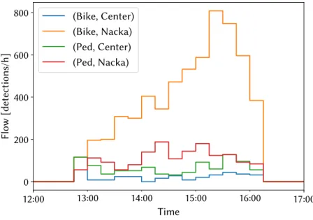
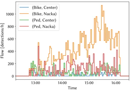
The afternoon commuter peak is clearly visible in the data, as can be seen in fig. 2, but the measurements was unfortunately aborted before the end of the peak. If the flow instead is aggregated over 2 min intervals it becomes obvious that it varies significantly over short times, as is clear from fig. 3, with several peaks with high volumes indicating that there may indeed be some interaction delay, even though the flows at the 15 min level are rater low.
12:00 13:00 14:00 15:00 16:00 17:00 Time 0 200 400 600 800 Flow [detections/h] (Bike, Center) (Bike, Nacka) (Ped, Center) (Ped, Nacka)
Figure 2: The flows aggregated over 15 min intervals. 3.3 ToDo Results
As mentioned above, in section 2.1, since cyclists do not strictly follow lanes, we need to make an assumption on how large the lateral separation between to cy-clists need to be for the following cyclist to be unconstrained by the leading. Here we take the same approach as Hoogendoorn and Daamen (2016) and simply as-sume a threshold, and furthermore asas-sume that this threshold is 0.5 m for all bicy-cles. Note that setting this threshold in the smaller end of the range of reasonable values is a conservative assumption; an underestimation of this threshold gives a overestimation of free cyclists and thus an underestimation of the desired speed and consequently also the delay and marginal cost.
When estimating the headway distributions, as summarized in section 2.1, we also need to set a threshold for how large a headway should be in order for it to surely be a free headway. Hoogendoorn and Daamen (2016) set this threshold to 4 s, due to a clear increase of the total headway distribution above an exponential
13:00 14:00 15:00 16:00 Time 0 200 400 600 800 1000 Flow [detections/h] (Bike, Center) (Bike, Nacka) (Ped, Center) (Ped, Nacka)
Figure 3: The flows aggregated over 2 min intervals.
distribution in the vicinity of 2 s. Here we use the same method as Hoogendoorn and Daamen (2016) to identify a suitable threshold: plotting the survival function of the headway distribution in semi-log axis and identify where it deviates from a straight line. In the data from Danviksbron the increase is less clear than in the data presented by Hoogendoorn and Daamen (2016), but seems to start some-where around 7 s, so we set the threshold to 8 s. This leads to an estimate of the distribution of free headways, scaled by the relative frequency of free headways. To obtain an estimate of the pdf of the desired following headways, an esti-mate of the pdf of the total headway distribution is needed. This can be achieved by constructing a normalized histogram, by kernel density estimation, or by as-suming a parametric form of the distribution and estimating its parameters using maximum likelihood estimation, or similar methods. To capture both the sharp peak of the distribution and that it vanishes as the headway size approaches zero, without over emphasizing noise for larger headways, we here choose to use an ad-hoc procedure of a normalized histogram with increasing bin width, which we interpolate linearly. The result is presented in fig. 4, where also the weighted pdf of the desired following headways is presented; this is simply the difference between the total distribution and the weighted distribution of the free headways. The probability that an observed cyclist with a given headway is following is given by the quotient between the distribution of preferred following headways and the total headway distribution. The result is presented in fig. 5.
0 5 10 15 20 25 30 Headway 0.000 0.025 0.050 0.075 0.100 0.125 0.150 0.175 0.200 Relative pdf All Free Following
Figure 4: The estimated headway distributions.
0 5 10 15 20 25 30 Headway 0.0 0.2 0.4 0.6 0.8 1.0 Probability of following
Figure 5: The probability that a cyclist with a given lead headway is following the bicycle ahead.
Kaplan-Meier method proposed by Hoogendoorn (2005), giving the estimated cdf presented in fig. 6, together with the empirical cdf of the observed speed distribu-tion. 0 2 4 6 8 10 12 14 Speed 0.0 0.2 0.4 0.6 0.8 1.0 Probability Actual Desired
Figure 6: The estimated desired speed distribution and the distribution of all observed speeds.
With the probability of following and the desired speed distribution as input, the expected delay for each observed cyclist can be calculated through eq. (4).
Probably the most intuitive measure of the delay is the relative delay, that is, the delay relative to the travel time at the desired speed. Aggregating the relative delay over two-minute intervals and plotting against the average flow in each interval gives the relation presented in fig. 7.
The total delay per unit traveled length is presented in fig. 8 together with the best fit curve of the form aq2. The best fit value of the parameter a is, in least squares sense, a ≈ 5.2 · 10−6h2/km. The total delay is given in the unit per kilometer, or more explicitly, h/(km· h), the delay, in hours, experienced per kilometer traveled by all cyclists passing during one hour.
The marginal delay caused by an extra cyclist per unit time is obtained by differentiation of the total delay, giving, assuming the form aq2for the total delay,
dδtot
dq = 2aq. (5)
Thus, the marginal cost of interaction delay is approximately given by 2aCq, where C is the value of time of the cyclists. Börjesson and Eliasson (2012b) es-timate the value of time for cyclists for short trips on a bicycle path to around 10 €/h, and the Swedish recommended standard value of time for cyclists on a
0 200 400 600 800 1000 Volume 0.00 0.05 0.10 0.15 0.20 Relative delay
Figure 7: The average relative delay of the cyclists in each two minute interval related to the average flow in the corresponding interval.
200 400 600 800 1000 Volume 0 1 2 3 4 5 6 7 Delay [/km] Mean delay aq2
Figure 8: The delay of all cyclists in each two minute interval related to the average flow in the corresponding interval.
bicycle path is 129 SEK/h (≈ 12 €/h) (ASEK, 2018). This would give a marginal cost of q· 1.3 · 10−4€h/km if the Swedish standard value of time is used. Assume that the traffic conditions are homogeneous over a stretch of 1 km and one hour. The cost of the delay over this stretch during this hour, induced by one additional cyclist per hour is 1.3· 10−4€ for each cyclist that passes the stretch during the hour.
3.4 Sensitivity analysis
The method proposed and applied in this paper is based on a number of assump-tions and simplificaassump-tions. The most concrete assumption is that cyclists are un-constrained by the preceding cyclist if their lateral distance is more than 0.5 m. This assumption is uncertain, and the assumed value of the threshold likely too low, and more detailed data are needed to investigate its accuracy. However, we can investigate the impact on the results of a slightly higher or lower value of this threshold.
The results of such a sensitivity analysis is presented in fig. 9, together with the results of a corresponding sensitivity analysis for the headway threshold, that is, the headway size above which it is assumed that there is negligible probability that a cyclist is affected by the preceding cyclist. This headway threshold was assumed to be 8 s since the total headway distribution starts to deviate slightly from an exponential distribution for shorter headways. However, this deviation is small and gradual, so the uncertainty is large.
The result of the method, in terms of the value of a, is evidently robust to changes in the lateral distance threshold; even when it is changed by as much as 40 %, the value of a is within 10 % from the original value. Variation of the head-way threshold, on the other hand, has a significant and complicated effect on the value of a. The sensitivity for an increase in the headway threshold in particular, is concerning since, in principle, the estimate of the free headway distribution should be more or less insensitive to increases above the threshold. However, as the threshold is increased the sample size of the data to estimate the parameters of the exponential distribution from decreases rapidly since it is close to exponential. Thus, any deviations from an exponential due to noise is rapidly becoming more influential as the threshold is increased.
4 Conclusions
The presented method can generally be used to estimate the interaction delay and its marginal cost in bicycle traffic. The application of the method to a case in Stockholm demonstrates that there exists significant interaction delay in the bi-cycle traffic, at least at the studied location. The studied location has a common
−0.4 −0.3 −0.2 −0.1 0.0 0.1 0.2 0.3 0.4 Rel. change in param.
−0.15 −0.10 −0.05 0.00 0.05 0.10 R el . c ha ng e in
a
Lateral threshold Headway thresholdFigure 9: The sensitivity of a to changes in the lateral position threshold and the headway threshold.
type of infrastructure, and the infrastructure is similar for rather long stretch up-stream, so the traffic at the site is unlikely to be affected by any particular feature, such as signals or other traffic control, upstream. The results are therefore ex-pected to be general. However, the significant uncertainties should be considered if applying the results.
5 Discussion
This paper considers how to use point measurements to estimate interaction delay in the observed traffic. Point measurements are inherently very limited in what type of information can be extracted, and this limits what can be investigated.
An important assumption in the method by Hoogendoorn and Daamen (2016) to estimate the desired speed distribution is that all desired speeds are indepen-dent. This means that it is assumed that no cyclists actually prefer to be in a following position, that is, it is assumed that there are no groups cycling together, and there are no cyclists following with the purpose of reducing the air resistance, as in cycling races. The occurrence of any of these two preferences will lead to an over estimate of the desired speed distribution. However, in commuting traffic the first effect is likely small, and the second effect is likely small in any non-racing traffic.
which in the case study is well motivated by fig. 1, from which it is clear that the studied cyclists, those traveling toward Nacka, are well separated from the pedestrians. Delay caused by direct interaction between a cyclist and a pedestrian is neglected by the method; if a cyclist is cycling slow due to the presence of a pedestrian it will be assumed that it is traveling at its desired speed. This will thus lead to an under estimate of the desired speed. However, indirect effects are captured by the method; the delay of cyclists queuing up behind a cyclist delayed by a pedestrian is of course included.
The results of the method by Hoogendoorn and Daamen (2016), fig. 5 and fig. 6, indicates that there is a significant difference between the observed and the desired speed distributions, and that the probability of following decreases to negligible levels after around 5 s. This is consistent with the assumed headway threshold of 7 s, and the results that there are significant delays at flows well below the capacity.
We also see, in line with Hoogendoorn and Daamen (2016), that there is sig-nificant ’noise’ in the probability of following as it approaches zero. This, in com-bination with the significant sensitivity of the result with respect to increases in the headway threshold, may indicate that some the assumptions underlying the method are not completely fulfilled, which could affect the accuracy of the esti-mates.
The most important source of uncertainty probably is that the analysis is per-formed on data from one afternoon at one location. Even though the site seems almost ideal for this type of investigation, we do not know if there were any spe-cial conditions during the day of the data collection that may have affected the traffic. Thus, even though the sensitivity analysis indicates that the marginal cost likely is within±20 % of the estimate, the true uncertainty is much larger, and can only be reduced by further data collection.
The main result of this study, the marginal cost, is given in terms of cost per increase in flow. This is a suitable measure only as long as the demand is below the capacity of the road, so that the actual flow increases as fast, or as least close to as fast, as the demand increases. This is an important implicit assumption of the presented method, that all measurement points in fig. 8 are, from a traffic flow theory perspective, on the uncongested branch of the fundamental diagram. Since the road is bidirectional, the capacity in the studied direction is dependent on the opposing flow, and also the pedestrian flow, so it is in principle possible that some of the points represent traffic states in the congested branch, although it seems unlikely. This could however potentially explain outliers in fig. 7 and fig. 8. A more careful analysis is required if the traffic state also could be on the congested branch of the fundamental diagram.
6 Acknowledgments
This research was funded by the Swedish Ministry of Enterprise and Innovation (’Uppdrag att fortsätta att utveckla forskningen om trafikens samhällsekonomiska kostnader’, N2017/01023/TS).
References
ASEK (2018). Analysmetod och samhällsekonomiska kalkylvärden för transportsek-torn, 6.1. Swedish Transport Administration.
Börjesson, M. and Eliasson, J. (2012a). “The Benefits of Cycling: Viewing Cyclists as Travellers rather than Non-motorists”. Cycling and Sustainability. Emerald Group Publishing Limited, pp. 247–268.
Börjesson, M. and Eliasson, J. (2012b). “The value of time and external benefits in bicycle appraisal”. Transportation Research Part A: Policy and Practice 46.4, pp. 673–683.
Buckley, D. J. (1968). “A Semi-Poisson Model of Traffic Flow”. Transportation Sci-ence 2.2, pp. 107–133.
Eriksson, J., Niska, A., Sörensen, G., Gustafsson, S., and Forsman, Å. (2017). Cyk-listers hastigheter: Kartläggning, mätningar och observation. VTI, Swedish Na-tional Road and Transport Institute.
Hoogendoorn, S. and Daamen, W. (2016). “Bicycle Headway Modeling and Its Ap-plications”. Transportation Research Record: Journal of the Transportation Re-search Board 2587, pp. 34–40.
Hoogendoorn, S. (2005). “Unified approach to estimating free speed distributions”. Transportation Research Part B: Methodological 39.8, pp. 709–727.
Kaplan, E. L. and Meier, P. (1958). “Nonparametric estimation from incomplete observations”. Journal of the American statistical association 53.282, pp. 457– 481.
Nilsson, J.-E. and Haraldsson, M. (2016). SAMKOST 2: redovisning av regeringsup-pdrag kring trafikens samhällsekonomiska kostnader. VTI, Swedish National Road and Transport Research Institute.