Environmental Kuznets Curve for Carbon Intensity : a Global Survey

Environmental Kuznets Curve for

Carbon Intensity

Bachelor’s thesis within Economics

Authors: Fernando Figueres Elena Popova

Tutor: Research fellow Lars Pettersson Ph.D Candidate Sofia Wixe

1

Bachelor’s Thesis in Economics

Title: Environmental Kuznets Curve for Carbon Intensity: a global survey

Author: Fernando Figueres

Elena Popova Tutor: Lars Pettersson Sofia Wixe

Date: June 2011

Subject terms: EKC; Environmental Kuznets curve; Carbon Emission Intensity; GDP per capita; fossil fuels; alternative and nuclear energy; rural population; life expectancy at birth

Abstract

This paper is a study of the connection of a number of factors- GDP per capita, fossil fuels, al-ternative and nuclear energy, rural population and life expectancy at birth to the Environmental Kuznets Curve. Two econometric approaches are applied in order to test whether the variables have a more pronounced linear or quadratic form. Four income groups of countries are investigated in order to check if the state of development plays a crucial role in environmental deterioration.

The results of the study point out that EKC does not apply for the chosen variables. From the regression for GDP, however, it can be concluded that EKC forms in 1990s.

2

Contents

Introduction ... 5

2

Background ... 7

2.3 Environmental Kuznets Curve ... 8

3

Empirical Framework ... 11

Emission intensity ... 11

Country income specification ... 11

Fossil Fuels Combustion... 11

Alternative and Nuclear Energy ... 12

Life expectancy at birth ... 13

Rural Population ... 14

4

Empirical Testing ... 16

4.1 Correlation between explanatory variables ... 16

4.2 Roberts and Grimes Methodology ... 16

4.3 Stern Methodology ... 16

4.4 Functional forms for this study. ... 17

4.5 Expectations ... 17

GDP per capita ... 17

Fossil Fuels Combustion ... 18

Alternative and Nuclear Energy ... 18

Life expectancy at birth ... 18

Rural population ... 18

5

Results and Discussion ... 19

5.1 Intensity Trends Worldwide Over Time ... 19

5.2 GDP per capita ... 19

5.3 Fossil Fuels share ... 22

5.4 Alternative and Nuclear Energy share ... 22

5.5 Life Expectancy at birth ... 23

5.6 Percentage of Rural population ... 23

5.7 Comparison of the results obtained by the two functional forms .. 25

6.Conclusion ... 26

7.

References ... 27

Appendix 1: Country list ... 30

Appendix 2 – Correlation tables ... 31

Appendix 3 - Regression Tables ... 32

3

Appendix 4 CO

emission by countries... 41

Appendix 5 – Fossil Fuel Consumption ... 45

Table of Figures

Figure 2 - Environmental Kuznets Curve ... 8

Figure 3 - Average intensity over time by income group. ... 19

Figure 4 - Sample cross sections for GDPc ... 21

Figure 5 - World energy source composition ... 22

Figure 6 - Rural population percentage ... 24

Figure 7 - Primary energy consumption ... 24

Figure 8 – Fossil fuel percentage of energy mix scatter plots ... 37

Figure 9 - Alternative and Nuclear energy scatter plots ... 38

Figure 10 – Life expectancy scatter plots ... 39

Figure 11 - Rural population (%) ... 40

Figure 12 - High-income group: CO2 emissions ... 41

Figure 13 - High-income group: CO2 emissions ... 41

Figure 14 - Upper middle income group: CO2 emissions ... 42

Figure 15 - Lower middle income: CO2 emissions ... 43

Figure 16 - Low income group: CO2 emissions ... 44

Figure 17 - Fossil fuel consumption for selected countries ... 45

Table of Tables

Table 2 - Country list... 30

Table 3 - Variable Correlations ... 31

Table 4 - Cross-sectional regression for GDP per capita as explanatory variable – Comparison between Stern and Roberts and Grimes methods ... 32

Table 5 - Cross-sectional regression for fossil fuels as explanatory variable – Comparison between Stern and Roberts and Grimes methods ... 33

Table 6 - Cross-sectional regression for alternative energy as explanatory variable – Comparison between Stern and Roberts and Grimes methods ... 34

Table 7 - Cross-sectional regression for life expectancy as explanatory variable – Comparison between Stern and Roberts and Grimes methods ... 35

Table 8 - Cross-sectional regression for rural population as explanatory variable – Comparison between Stern and Roberts and Grimes methods ... 36

4

Abbreviations

EKC Environmental Kuznets Curve CO2 Carbon Dioxide

GDP Gross Domestic Product

GDPc Gross Domestic Product per Capita

GHG Green House Gases

UNDA United States Department of Agriculture NIFA National Institute of Food and Agriculture

Variable names in the regression tables are named with the following convention.

Natural logarithm Squared Variable name year

l_ Sq_ foss =fossil fuels share 2 digit

alt=alternative and nuclear energy share

rur=rural population share Life=life expectancy at birth Gdpc=GDP per capita

5

Introduction

Currently the world is struggling with two major problems. On one hand, billions live in absolute poverty. On the other, global warming, resource depletion and environmental degradation have forced the world to rethink how it will supply a quality life to an ever increasing population.

Economic development and environmental sustainability have been seen as two important but mutually exclusive goals. The Environmental Kuznets Curve (EKC) proposes that this is not the case and that development ultimately leads to a better environment. The EKC is an inverted U-shaped re-lationship which demonstrates that after a certain income threshold is achieved, environmental degra-dation starts to decrease while income continues to increase. It may be that countries become more environmentally friendly due to the fact that at later stages of development they are more aware of and interested in reducing environmental pressure (Bo 2011). Even though pollution and affluence are positively correlated to a certain point (Grossman & Krueger 1991), they do not increase at the same pace.

The complex and important relationship between development, equity, and environment can be easily seen in the following quote: “The growth rate in emissions is strongest in rapidly developing economies, particularly China. Together, the developing and least-developed economies (forming 80% of the world’s population) accounted for 73% of global emissions growth in 2004 but only 41% of global emissions and only 23% of global cumulative emissions since the mid-18th century. The re-sults have implications for global equity.”(Raupach,Marland and Ciais, 2007)

This paper studies several indicators of development along with GDP per capita (GDPc) in or-der to test whether these, along with carbon intensity have a statistically significant relationship and EKC behavior. We have chosen carbon intensity as a measure of environmental pressure since it shows the level of efficiency with which countries are driving their economies. Additionally, the un-derlying variables of carbon intensity, GDP and C02 emissions, are widely available for a large number

of countries and years. Separate regressions will be run utilizing fossil fuel share, alternative and nuc-lear energy share, rural population share, life expectancy at birth and GDP per capita as explanatory variables. By using these explanatory variables, this paper will attempt to detect the EKC effect for development indicators other than GDP.

A number of studies conducted so far indicate a relationship between some pollutants and eco-nomic growth. Lead, particulates, sulfur oxides and nitrogen oxides all exhibit a positive correlation between environmental degradation and affluence for the OECD – countries (de Bruyn 1998) . The problem of environmental degradation is usually attributed to industrial production and consumption. On the other hand, when people become richer and also better informed about the negative effects on environment, they are more inclined to spend on products with less unfavorable influence on na-ture.

Countries with high income and technological levels focus on a less pollution intensive produc-tion, while poorer countries engage in heavy manufacturing and contribute a lot to the worldwide pol-lution rates.

International trade allows for such structural changes in the economy since what is not pro-duced within the countries’ borders can be obtained from the market. Another aspect of trade is that in open to trade economies the pollution is less in comparison to closed economies. This is probably due to the fact that open economies engage mainly in labor intensive activities while closed countries – on capital intensive ones. (Hettige et al. 1992; Grossman & Krueger 1995)

6

People gathering into cities and forming agglomerations has turned out to be more efficient and less degrading when environment is concerned. Densely populated urban areas can benefit from al-ready built infrastructures which reduce transportation costs for both people and products reaching final destionations.”Cities also offer opportunities to manage a growing population in a sustainable way.”(United Nations Environment Programme 2002)

Also, strict and legislation is usually adopted in more wealthy countries which additionally im-proves the condition of the environment (Bradford ,Schlieckert and Shore , 2000).

1.1

Purpose

The aim of this paper is to investigate which variables can possibly explain carbon emission in-tensity and whether they follow the Kuznets curve. Since EKC is not an exact model different studies have reached different conclusions. This study adopts two functional forms in order to test the con-sistency of the results obtained with the different variables. The first is proposed by Roberts and Grimes (1997), while the later is suggested by Stern (2004). We will study a sample of 73 countries1

from 1972 to 2005.

1.2

Limitations

As laid out the in the literature survey, the EKC is an empirical regularity without a standardized model or variables. As such, its study still lacks from comparability and consensus among scholars as to how the effect forms and how to study it. Economic activity is not perfectly captured in GDP per capita. Although CO2 accounts for a large portion of anthropogenic green house gases and serves as a

proxy for energy use, pollution is a complex issue and spans a plethora of polluting agents. By choos-ing standardized macroeconomic indicators such as CO2, rural population and so forth, we are able to

obtain a long term view of the EKC but at the same time, these variables must be understood as proxies of a much more complex underlying process.

The empirical study of the EKC has several econometric difficulties. The main problems are heteroskedasticity, simultaneity and omitted variables (Stern 2004). Stern points out “regression resi-duals are heteroskedastic with smaller resiresi-duals associated with higher total GDP and population.” Neglecting the simultaneity issue, one might reach a conclusion about causality direction- increase in GDP is entailed by increase in pollution, when in reality it might be the opposite or not related (Stern 2004).

7

2

Background

2.1

Theoretical Framework

The EKC is not a clear cut model based on precisely determined variables and mathematical re-lationships. On the contrary, it is an empirical phenomenon with varying level of significance across the many time periods, regions, pollutants and other factors which have been studied. Our paper, like others before it, attempts to test a set of new variables in order to increase the understanding of the relationship between development and environmental degradation.

Conventionally the EKC has used a monetary measure, such as GDP per capita, as an explana-tory variable since the regressand already includes GDP in the intensity measure; it is possible to test if other development indicators follow the EKC relationship.

Based on previous research efforts on the subject, we may summarize the factors which influ-ence the relationship between development indicators and pollution under the following general prin-ciples.

1. As income increases the demand grows for environmental quality but also the resources ne-cessary to supply it (Panayotou 1997b).

2. People have a greater incentive to deal with things that affect them directly. This has been shown from the studies which demonstrate that the drinking water quality has a lower turning point than CO2, for example (Levinson 2008).

3. Unless properly internalized under a democratic and transparent system with well informed players, production of externalities will not be socially efficient (Torras, 1998).

4. Those that are least capable of bearing the transaction costs associated with the negotiation of externality production and its control will bear most of the externalities (Boyce 1994).

5. Efficiency and output increase practically monotonically through time. There are important asymmetries in the time and scale effects throughout the development process which may lead to nonlinear income/pollution relationships (Stern 2004).

6. People with higher income tend to live in cities and longer (Brakman 2009).

7. People with higher income pollute more, especially with regard to greenhouse gases (Brakman 2009).

8. As per capita income increases there is a clear decline in agricultural output coupled with an increase in the output of the service sector (Brakman, 2009).

9. On a world scale there is a strong correlation between level of urbanization and per capita in-come (Brakman 2009).

8

2.2

Kuznets Curve

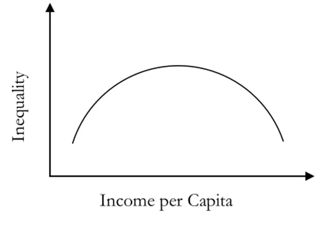
The idea of the Kuznets curve first originated in a paper published in 1955 by Simon Kuznets on the relationship between economic growth and inequality. He postulated that inequality increased with economic growth but only until a point, after which inequality began to decrease as income con-tinued to increase (Kuznets 1955). This effect forms an inverted U-shaped relationship with a meas-ure of income in the X axis and inequality in the Y axis,as shown in Figmeas-ure 1.

2.3

Environmental Kuznets Curve

Grossman & Krueger (1991) decided to adapt this concept to environmental impact. In their view, environmental impact, like inequality should increase with income up to a point at which it be-gins to decrease while income continues to increase. This effect is attributed to the possibility of effi-ciency improvements due to technological advances. With increase in income, investment in research and development also increases. The concept was further popularized by the World Bank’s 1992 World Development Report (1992). Since then numerous studies have been done to investigate the relationship between economic development and some measure of pollution Boyce 1994; Magnani 2000; Selden & Song 1994; Roberts & Grimes 1997; Torras 1998 among many others.Error! Refer-ence source not found. illustrates the EKC.

Figure 2 - Environmental Kuznets Curve

In

eq

ua

lit

y

Income per Capita Figure 1 - Kuznets Curve (1955)

9

One of the first papers to further study the EKC was written by Hettige, Lucas and Wheeler (1992). In it, they studied the relationship between stages of development, pollution intensity, GDP and industrial output. They hypothesized that there are three basics stages of industrial development. They defined them as “agro processing and light assembly” which they classify as low in toxic intensi-ty; “heavy industry” which is high in intensity and finally high-technology industry” which is also low in toxic intensity. Their analysis concluded that there was an inverse U-shaped relationship between pollution intensity per GDP but such pattern was not found when industrial output was the explana-tory variable. Based on this ambiguity they concluded that the GDP-based intensity relationship was based on structural shift from industry towards a more service oriented economy. As the shift oc-curred, more toxic sectors were transferred to the emerging economies. Interestingly, they point out that the pattern reversal for the OECD countries was brought about by the advent of stricter envi-ronmental controls during the 1970’s and 1980’s.

Other studies have acknowledged the possibility of an EKC but predict that the turning point is too far in terms of time and level of income that has not practical relevance (Miah, Masum, Koike & Akther 2011a; Selden & Song 1994). A research on Kuznets in Bangladesh estimates that the country is at the upward sloping region of the EKC. This study examines whether Kuznets is applicable to the deforestation which Bangladesh experiences at a large scale. It concludes that the situation very much resembles a Kuznets curve and claims that the turning point at which deforestation will start to de-crease is further in the future (Miah et al., 2011).

There has been substantial development in the study of the impact of factors such as institu-tional development, corruption and income equality on the EKC. Leitão (2010) tested whether cor-ruption had an influence on the EKC turning point for sulfur emission. He used a large sample of countries in different levels of development. Following the methodology proposed by Bradford,Scliekert and Shore (2000), he found that sulfur emissions follow EKC and most important-ly, that corruption has a significant effect on the turning point level of income. Esmaeili & Abdollahzadeh (2009) found that oil producing countries with more equal distribution of income and democratization reduce the rate of oil exploitation. Clement & Meunie (2010) have found also that in-come equality through the Gini index has a Kuznets relationship for water pollution in developing countries. Barrett & Graddy (2000) have also found significant correlation between political freedom and environmental improvement. Along the lines of previous research they motivate this effect to the “induced policy response”. This effect occurs when people increase their demand for environmental quality as income increases. In their study, they argue that the political influence of such demand will depend on the political freedom and influence the people have on their government.

Studies have indicated that the implementation of better policies is also closely related to im-provements in the environment at both low and high income levels. Enhanced property rights regula-tions, enforcement of contracts and environmental regulations can play a major role and even counte-ract the growth in population and production levels.

Several scholars acknowledge the Kuznets effect but argue that it is not due to countries passing by different stages of development but due to a small number of rich countries improving while a number of poor countries worsening in terms of carbon intensity (Roberts & Grimes 1997). Stern (2004) argues that EKC does not exist. It is an effect caused by the difference between the scale and time effects of economic activity between developed and developing countries. It seems the EKC is a mix of factors in scale, composition and technique (Brock & Taylor 2004).

Iwata H., Okada K. and Samreth S. (2010) find the Kuznets curve works for nuclear power in France. The ever-increasing role of nuclear power has also been subject of study in the Kuznets

rela-10

tionship. Although nuclear power has a bad reputation, its carbon footprint is much lower than that of coal or oil. France alone account for 3.3% of global GDP while at the same time it is to blame only for 1.5% of the world’s emissions (World Resources Institute, 2005).

Environmental dumping has been one of the supposed factors behind the parabola-like rela-tionship between pollution and affluence for some countries but (Ehrhardt-Martinez K., Crenshow E., Jenkins C. 2002; Grossman & Krueger 1991) have found little evidence that environmental dump-ing is a significant factor in the EKC formation.

The overall results of the studies produced over the years point to lower turning point estimates for pollutants that directly affect people’s health such as coliform bacteria in drinking water or sulfur emissions. On the other hand, pollutants with little direct impact have turning points much further in the future or at higher incomes (Cole et al. 1997; Levinson 2008).The justification for this should stem from one of the primary drivers of the EKC, people’s demand for a better environment as their utility from consumption diminishes and the environmental degradation increases, those agents which most directly diminish quality of life are dealt with firstly. C02, among other greenhouse gases, is colorless,

odorless and basically non-toxic. It is only through long term scientific research that is has been iden-tified as a pollutant due to its climate altering effect (IPCC 2007).

A factor of inter-temporal trade in between environmental quality and capital accumulation may be in play. For example, if a new island is discovered and turning it into a civilized place and building its infrastructure begins now, environmental depletion will be tremendous. At the early stages, con-struction on the island starts from scratch and exploitation of resources occurs at a very high pace and low efficiency. Gradually, this pace is reduced since some progress is achieved already and the envi-ronment has time to recover.

11

3

Empirical Framework

The majority of previous studies in the field focus on measuring the emissions of the GHG they have chosen rather than the intensity of these emissions.We would like to focus on the speed and trend with which CO2 emissions progress.Also it is worth noting that the usual variable against which

pollution is measured is GDP per capita.Even though a purely monetary indicator is a good mea-surement of economic development and therefore can explain GHG emissions,it is also interesting to expand the study with variables which can tell a little more about the process of polluting such as fossil or alternative and nuclear energy production.Variables such as life expectancy at birth and rural population give a fair picture of the economic structure within a country and since we are interested in different levels of development we will include them in our paper.

Emission intensity

The environmental degradation variable used throughout the paper is defined as follows: “Emission intensity is the level of GHG emissions per unit of economic activity, usually measured at the national level as GDP.”Carbon emission intensity is a compound of two measurements: the ener-gy mix and the fuel mix of a country. Since these two are very different in every single country, emis-sion intensity also varies a lot (World Resources Institute. 2005).According to (Roberts & Grimes 1997) there are four major reasons why carbon intensity can account for the threshold at which the Kuznets curve changes its shape: 1) carbon dioxide is the main factor behind greenhouse warming, 2) before CO2 was considered harmless to the environment, 3)there is no amount of CO2 needed to be

emitted in order for an economy to have a certain size or population, 4) data on CO2 is available.

Country income specification

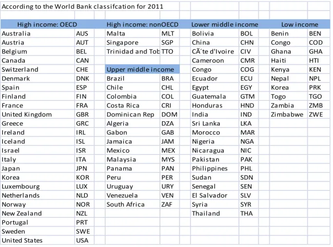
Part of the analysis is based on comparing countries in different stages of development. We have followed the World Bank’s classification based on income per capita which is also used in the Roberts and Grimes paper.“Economies are divided according to 2009 GNI per capita, calculated us-ing the World Bank Atlas method. The groups are: low income, $995 or less; lower middle income, $996 - $3,945; upper middle income, $3,946 - $12,195; and high income, $12,196 or more.” (World Bank 2011). The classification was made based on the 2011 income levels and were not adjusted through time.

Fossil Fuels Combustion

Due to the tremendous increase in energy demand (70% since 1971), the increase in GHG emissions also intensifies. Fossil fuels are coal, natural gas and oil. “Fossil fuels supply roughly 90 per-cent of the world’s commercial energy; energy-related emissions account for more than 80 perper-cent of the carbon dioxide (CO2) released into the atmosphere each year. By 2010, IEA projects that global

energy consumption – and annual CO2 emissions – will have risen by almost 50 percent from 1993

levels”(World Resources Institute, 2005). There are still other issues that add up to the disadvantages of fossil fuels except for purely environmental concerns. A good example of that is national security. Due to the uneven distribution of fossils among different countries, the ones with more deposits can influence international politics. The Persian Gulf War, for instance, led to the intervention of US mili-tary forces in order to guard for possible deficiencies of oil. It is also noteworthy to mention that this can be entailed by oil price speculations which the world has already experienced (Union of Concerned Scientists 2010). The share of fossil fuels should also decrease over time as there has been a tremendous improvement in the production handling and use of hydrocarbon throughout history,

12

double digit improvements in efficiency are common and thus, we would like to know if the EKC is followed.

Since this is one of the primary sources of environmental pressure, it seems reasonable to test if it follows the Kuznets curve. If it decreases over time after a threshold is reached, then the hypothesis of Krueger and Grossman of Environmental Kuznets Curve is justifiable.

Alternative and Nuclear Energy

Alternative energy is vital for the survival of our planet. Since, fossil fuels are the major source of anthropogenic GHG emissions, reducing fossil fuel use is critical in diminishing our effect on the world’s climate. There are a number of interpretations of the term alternative energy, varying mainly on whether they include or exclude nuclear energy. “Alternative energy refers to energy sources that have no undesired consequences such as for example fossil fuels or nuclear energy. Alternative energy sources are renewable and are thought to be "free" energy sources. They all have lower carbon emis-sions, compared to conventional energy sources. These include biomass energy, wind energy, solar energy, geothermal energy, hydroelectric energy” (Alternative Energy Institute 2011). ”Clean energy is non-carbohydrate energy that does not produce carbon dioxide when generated. It includes hydro-power and nuclear, geothermal, and solar hydro-power, among others.”(World Bank, n d). For this paper, we will use the World Bank definition.

The main disadvantage of alternative energy is that even if the current pace of research and im-plementation continues, this source will not be able to account for more than 6% of global electricity by 2030 (Henriquez A. 2008).Therefore, alternative energy providers cannot meet the needs of mod-ern society at the current time.

Nuclear energy is one of the main options humanity has in order to provide for electricity supply and production needs. It has a handful of benefits with regard to nature since it pollutes much less than fossil fuels and after usage is safer to store underground than it used to be. The source for nuclear energy is the chemical element Uranium, which is abundant under the earth surface and sea water and is needed in small quantities. This implies that nuclear energy production is not susceptible to such shortages as the oil embargo of the 1970’s, for instance. The waste produced afterwards is in little amounts and with current technologies manageable to collect and dispose (U.S. Nuclear Waste Technical Review Board 2010).

When nuclear energy is considered there is no threat of exhausting existing resources and there-fore it can be relied upon in the long run. All other existing types of producing energy depend largely on nature; let it be sun, wind, water or fossils. Once the planet runs out of petroleum, for example, or the wind does not blow, the energy supply will be interrupted. (Nuclear Energy Institute 2011)

The main advantage of nuclear plants is that they have the lowest impact on the environment. In most countries the electricity tax includes also the price for underground disposal of the waste. Thus, neither the production, nor the storage of nuclear energy leads to any negative externalities. (Toth 2011)

Due to some accidents in the past nuclear energy has been deemed as extremely dangerous for people and nature. After the breakdown of Chernobyl and the radiation cloud spread, nuclear energy was condemned. A thorough investigation of the causes and effects followed and it revealed that the poor quality of the reactors was the reason for the tragic incident. In terms of safety, technologies have greatly improved the quality of reactors in use today. Nowadays, better constructed and more

ef-13

ficient reactors are the standard. Occurrences such as earthquakes and other natural disasters are tak-en into account whtak-en designing nuclear plants or storage compartmtak-ents. (Ingram 2005)

The expenditure for building a nuclear plant is still greater than for a natural gas or coal one. However, once built the plant can be more efficiently run .The construction periods for nuclear plants are shorter, so it can be put into practice more quickly. (Henriquez A. 2008)

Having in mind all the technological advances,it is still virtually impossible to build an entirely secure nuclear power plant and some possibility of reactor failure will still remain.The storage of nuc-lear waste is also improving but the risk remains.According to the United States Environment Protec-tion Agency standars 10 000 years is the minimum period during which nuclear waste must be taken-taken care of.Another disadvantage of nuclear plants is that they often are the target of terrorist at-tacks and plants are not developed in a way to withstand such atat-tacks.Also nuclear waste resulting from the energy production can be used for nuclear weapons development. (Nuclear Information and Resource Services 2011)

Life expectancy at birth

Longevity is “an indicator of a country’s overall health” (Conference Board of Canada 2011). It demonstrates the quality of life in a country. The better developed a country, the better standard of living its citizens enjoy. To draw a comparison, the life expectancy in Sweden (an example of a coun-try with a high standard of living) for 2010 is 81years, and in Sudan (an example of poor quality of life conditions) is 58 (World Bank Staff 1992). The life span at birth is an estimation of how many years a new born infant will live if the trends in the country of origin do not change significantly over time (World Bank).It demonstrates the pattern across all age groups –children, adolescents, adults and elderly. Research indicates that there is a close connection between economic growth and life expec-tancy(Lorentzen et al. 2008). In poor areas with no adequate health care and access to sanitation, where the average life span is low, people do not have the incentive to invest in education since they will not live long enough in order to enjoy the benefits of it. Since they do not invest in human capital the development of the economy is hindered due to the lack of highly -qualified professionals. In the paper “Death and Development” (Lorentzen P., Mcmillan J. and Wacziarg R., 2008) it is clearly dem-onstrated that adult mortality leads to further poverty.

The Chernobyl accident can serve as a very good example of how people’s attitudes to eminent death can trigger them to act irresponsibly. At the time of the reactor failure, it was recorded that population in the vicinity was firmly convinced they were to die due to prediction of high radiation le-vels. Their behavior was characterized with “reckless conduct, such as consumption of mushrooms, berries and game from areas still designated as highly contaminated, overuse of alcohol and tobacco, and unprotected promiscuous sexual activity.”(Lorentzen et al. 2008)

According to Soares (2008) an increase in life expectancy affects the investment in human capi-tal and reduces birth rates. In Africa, where a large share of the world’s poorest countries with lowest life span is situated, the fear of AIDS and other diseases act as a discouragement for people to devote their efforts to education. Since these are life - long conditions from generations to generations the at-titudes perpetuate and do not seem to undergo any positive change. People are more inclined to in-vest in short run benefits for it is uncertain whether they will be able to gain any in the long run. Par-ents tend to have more children because of the high risk of premature death instead of having fewer and focus on their upbringing and education. Empirical research points out that Sub-Saharan African countries have slowed down their development so much that between 1960-2000 the discrepancy be-tween their income per capita and the rest of the world has doubled .It is also worth noting that out

14

of 40 countries with highest death toll all but three are in Africa.”Per capita income is significantly as-sociated with the mortality rate, and mortality is significantly asas-sociated with growth.” (Lorentzen et al., 2008).This observation shows that longevity is closely related to economic growth and therefore to emissions as well since they occur where heavy manufacturing is present.Sometimes life expectancy at birth will be simply referred to as life expectancy for conciseness.

Rural Population

Not many studies have been devoted to the impact of population on environmental degrada-tion. The majority of them are focused on the influence wealth exerts on environmental quality. Pop-ulation can be one of the main (though not necessarily always) drivers of increased production since the aggregate demand of a country’s inhabitants leads to increase in supply. Experiments conducted before point out that population has a crucial impact on carbon intensity. Anqing Shi (2001) recogniz-es the fact there must be significant relationship between carbon emissions and growth in population: “The impact of population growth on environment quality is obvious. Each person in a population makes some demand on the energy for the essentials of life – food, water, clothing, shelter and so on. If all else is equal, the greater the number of people, the greater the demands on energy.” In the paper “Population growth and global carbon dioxide emissions” Shi reaches two very important conclu-sions: increase in population goes hand in hand with global CO2 emissions and rising income levels

are characterized by upward shift in pollution.

In order to conduct the study, Shi constructs panel data sets for 93 countries for the time pe-riod 1975-1996. Shi divides the countries into four categories according to their income level follow-ing the classification of the World Bank: 26 low income countries, 24 lower middle income countries, 14 upper middles income countries and 29 high income countries. In the model carbon emissions stand for burning fossils fuels in the manufacturing sector and for the production of cement. Wealth is measured in terms of real GDP per capita in constant price (1995 U.S. dollar).Energy efficiency is measured as the ratio of real GDP in 1955 U.S. dollars to commercial energy used. In one single model the author combined the effects of population growth, income level and energy efficiency. The results point out that:

 1% increase in population entails a 1.28% increase in carbon emissions on average.

 Population growth in developing countries produces larger impacts on pollution in compari-son to developed ones.

 Global emissions will reach 12.72 gigatons by 2025 if population increase follows the pattern of medium growth estimated by the UN and GDP increases with 1.9% per year.

 In absolute terms more affluent countries pollute as much as half all global emissions; low income countries exhibit a faster increase in emissions.

 In relative terms the share of high-income countries decreases (from 69.7% in 1975 to 54.9% in1996) and that of low-income countries is on the rise (from 13.4%in 1975 to 25.3%in 1996)

 Population increases in descending order as follows: low-income, low middle income, upper middle income to high income countries

In conclusion, Shi advises policy-makers to take these findings into consideration when discuss-ing possibilities for reducdiscuss-ing carbon emissions together with affluence.

According to Dietz & Rosa (1997) the impact of population is proportional to its size across a number of countries and this is the trend for the decades ahead. They conducted a study of the

im-15

pact of three factors: wealth, population size and technological level on environmental deterioration. For that purpose they used a stochastic IPAT model, Impact =Population * Affluence * Technology. Dietz and Rosa found out all of the three were actual driving forces and were interconnected. Their findings refute the possibility that population growth does not affect pollution. On the contrary, ac-cording to their results: ”the impacts of population are roughly proportional to its size across the range of population size and will characterize most nations over the next few decades.”

Rural population was chosen as a variable because it is one of the major differences between in-dustrialized and emerging economies. The share of rural population shows the structure of a country’s economy. This is due to the fact that advanced economies have incorporated state-of-the–art tech-nologies in their farming and agriculture and a large number of workers in the fields or for breeding stock is not necessary anymore. For example, in the USA less than 2% of the work force is in the agriculture sector and only 17% of the population remains in the rural areas (UNDA/NIFA 2011).This is the reason why a large proportion of the population migrates to urban areas. Less devel-oped nations, to the contrary, need a lot of laborers to grow their crops and produce food. That is why a large percent of the population is concentrated in rural areas.

16

4

Empirical Testing

In order to test whether the EKC forms for each variable, we will use yearly cross sections. As methodological aspects of the EKC are sometimes put in doubt, we have chosen two competing functional forms in order to test the robustness of our estimates. The first is proposed by Roberts and Grimes (1997) in which only one of the variables is squared, the other, by Stern (2004), takes the loga-rithm of the quadratic variable before it is squared.

This comparison was decided upon due to the fact different studies reach different conclusion which might be as a result of the functional form used.According to the study carried out by Roberts and Grimes, EKC forms but at the same time their econometric model has received some criticism (Mcnaughton and Lee, 1998).The fact that they log only the linear parameter of GDP puts into doubt the soundness of their empirics and the credibility of their results.However,in the paper criticizing the econometric model of Roberts and Grimes (1997), Mcnaughton and Lee conclude “Results… sup-port the main point of the paper.”Another reason why we chose their functional form is that they deal with CO2 intensity and not CO2 emissions as the majority of other studies. In order to be more

credible we include another functional form proposed by Stern (2004),which seems to be more eco-nometrically sound and test if the results differ substantially.

4.1

Correlation between explanatory variables

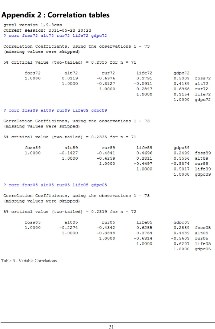
Since all the selected explanatory variables represent an aspect of human development, it is nat-ural to suspect substantial correlation which would undermine the usefulness of studying them sepa-rately. We have calculated correlation tables for our explanatory variables for the beginning, middle and final year of our sample. As can be seen in Appendix 2, Table 3 most correlation coefficients fall under 0.5. It should be possible to have different results from each variable.

4.2

Roberts and Grimes Methodology

The econometric equation for each yearly cross-section in the Roberts and Grimmes (1997) pa-per can be expressed as:

(1) in which:

Tonnes of emissions per year GDP per capita

Stochastic disturbance

In each case the study examines the behaviour of the R2_{, standard errors and significance of the}

parameters for the selected variable across time. Based on these we should see whether the Kuznets curve forms for the selected variables.

4.3

Stern Methodology

Following the standard EKC as proposed by Stern (2004) we can model the EKC with the fol-lowing relationship:

17

(2)

E Emissions ln Natural logarithm P Population i Region

GDP Gross Domestic Product t Year

The main difference between the two approaches lies in that the squared term is logged as well. Unlike Stern, we will use yearly cross-section analysis rather than panel data. This paper will use Rob-erts and Grimes yearly cross section method but will use the functional form used by Stern without the α or terms.

4.4

Functional forms for this study.

Our method is OLS regressions with robust standard errors.We will adapt both functional forms in the following way:

Roberts & Grimes (3)

Stern (4) I Carbon intensity V Explanatory variable ln Natural logarithm Error term s Country Data Sources

Our data covers yearly measurements from 1972 to 2005. Data for GDP per capita, fossil fuel share and alternative fuel share were obtained from the World Bank statistical database (databank.worldbank.org). Statistics on life expectancy and rural population were obtained from the World Resources Institute database (www.wri.org). GDP figures are based on current USD for ease fo comparison and C02 emissions are measured tonnes.

4.5

Expectations

GDP per capita

According to Roberts & Grimes (1997), GDP per capita should exhibit a more pronounced li-near relationship to carbon intensity at the beginning of the examined period. However, over time this trend changes to inverted U shaped parabola or more Kuznets -like behavior due to the increasing

18

significance of the quadratic coefficient against the linear coefficient. In order to have a downward parabola the coefficients should be negative.

Fossil Fuels Combustion

Having in mind that fossil fuels are the main source of anthropogenic carbon emissions, it is expected that there is an upward sloping linear relationship. Nonetheless, since efficiency is not meas-ured in absolute values of pollution and intensity is the main interest, it could be expected an EKC to form due to the output gains as a greater percentage of the economy is powered by fossil fuels.

Alternative and Nuclear Energy

Although alternative energy sources have an obvious environmental advantage, only nuclear energy is a strong contender to oil when considering reliability and cost. Alternative energy sources are still a novel development with major price disadvantages and high uncertainty with regard to supply. For most countries, it represents a small portion of their energy mix. We should expect little or no significant positive impact on intensity as alternative sources are implemented.

Life expectancy at birth

According to the general Kuznets relationship, a measure of development should first induce higher levels of pollution which decrease at a turning point. As life expectancy increases people are more willing and able to invest in human capital until some point in time with the increase in life ex-pectancy entails increase in GDP and as we mentioned earlier, with the rise of GDP there is a rise in pollution until the moment when production becomes more efficient due to the implementation of new technology. Then, although GDP continues to increase it becomes negatively correlated with emissions and the same applies for life expectancy. During the period 1972-2005 the life span for the four groups of countries has increased as follows: in low income countries it increased from 50 to 55, in lower middle income group the increase is from 53 to 65, in the upper middle income group and high income group the change is from 61 to 71 and from 70 to 79 respectively. Obviously, longevity has increased substantially with the exception of the low income countries.

Rural population

The effect of rural population is unclear. Rural population is a major indicator of the industriali-zation process and the level of development. On one side, a high rural share should indicate predo-minance of agriculture and low industrial development which should be correlated with low carbon intensity. But at the same, the low development levels should yield equally low amounts of output. As countries develop and the rural population moves to the cities, output should increase, but due to the need to build the infrastructure and other initiation problems intensity should be higher. As the urban rationalization process proceeds intensity should decrease.

19

5

Results and Discussion

5.1

Intensity Trends Worldwide Over Time

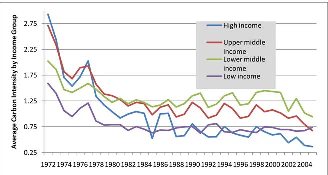
The change in intensities over time of individual countries does not seem to have an inverted u shaped trajectory, but when each cross-section is viewed as a whole, the EKC does form. This should imply that countries with lower per capita incomes have increasing intensities while those with high incomes have decreasing intensities. The underlying motives for this may be several (change in pro-ductions functions, preferences, income among others), due to the heterogeneity of the sample. After plotting the four income groups against time (Figure 3) the following patterns are ob-served: generally speaking carbon intensity is decreasing for all countries. The high-income group ex-hibits the least CO2 intensity rates which are in line with Kuznets prediction. They are followed by the

lowest income countries which can possibly be due to the fact that their manufacturing sector is still well behind in comparison with developed countries. The trend for the upper middle income group is also decreasing in intensity even though the line is above the one presenting the high income group of countries. In the future they will probably reach the state of the high income group and also become more efficient. The lower middle income group shows improvements in its production efficiency and is expected to further reduce its pollution intensity in the long run. Thus, all four groups are in line with Kuznets expectations for GDP per capita.

Figure 3 - Average intensity over time by income group.

5.2

GDP per capita

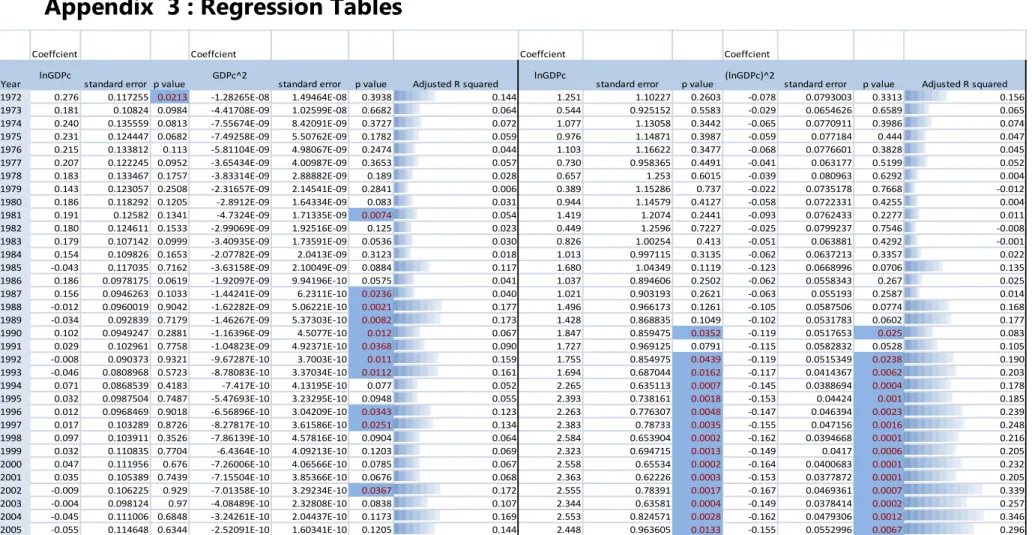
The experiment’s outcome replicates the results obtained by Roberts & Grimes (1997). Our li-near parameters, (log transformed), presented below in Table 1, become less significant while the quadratic increase in significance. This indicates that at the beginning of the studied period the corre-lation is linear but over time becomes curvilinear.After 1987 the EKC forms. Since 1990 both

para-0.25 0.75 1.25 1.75 2.25 2.75 1972 1974 1976 1978 1980 1982 1984 1986 1988 1990 1992 1994 1996 1998 2000 2002 2004 A ve ra ge C arb o n In te n si ty b y In co m e G ro u p High income Upper middle income Lower middle income Low income

20

meters in Stern’s regression become significant and the R2 _{increases slowly over time. This indicates a}

transformation of the relationship between GDP per capita and carbon emission intensity from linear to quadratic. Therefore,Stern’s functional form yield results that imply the existence of EKC and pro-vides more efficient estimates.

Year GDPc^2 Adjusted R squared lnGDPc (lnGDPc)^2 Adjusted R squared

1972 0.276 ** -1.2827E-08 0.144 1.251 -0.078 0.156 1973 0.181 * -4.4171E-09 0.064 0.544 -0.029 0.065 1974 0.240 * -7.5567E-09 0.072 1.077 -0.065 0.074 1975 0.231 * -7.4926E-09 0.059 0.976 -0.059 0.047 1976 0.215 -5.811E-09 0.044 1.103 -0.068 0.045 1977 0.207 * -3.6543E-09 0.057 0.730 -0.041 0.052 1978 0.183 -3.8331E-09 0.028 0.657 -0.039 0.004 1979 0.143 -2.3166E-09 0.006 0.389 -0.022 -0.012 1980 0.186 -2.8912E-09 * 0.031 0.944 -0.058 0.004 1981 0.191 -4.7324E-09 *** 0.054 1.419 -0.093 0.011 1982 0.180 -2.9907E-09 0.023 0.449 -0.025 -0.008 1983 0.179 * -3.4094E-09 * 0.030 0.826 -0.051 -0.001 1984 0.154 -2.0778E-09 0.018 1.013 -0.062 0.022 1985 -0.043 -3.6316E-09 * 0.117 1.680 -0.123 * 0.135 1986 0.186 * -1.921E-09 * 0.041 1.037 -0.062 0.025 1987 0.156 -1.4424E-09 ** 0.040 1.021 -0.063 0.014 1988 -0.012 -1.6228E-09 *** 0.177 1.496 -0.105 * 0.168 1989 -0.034 -1.4627E-09 *** 0.173 1.428 -0.102 * 0.177 1990 0.102 -1.164E-09 ** 0.067 1.847 ** -0.119 ** 0.083 1991 0.029 -1.0482E-09 ** 0.090 1.727 * -0.115 * 0.105 1992 -0.008 -9.6729E-10 ** 0.159 1.755 ** -0.119 ** 0.190 1993 -0.046 -8.7808E-10 ** 0.161 1.694 ** -0.117 *** 0.203 1994 0.071 -7.417E-10 * 0.052 2.265 *** -0.145 *** 0.178 1995 0.032 -5.4769E-10 * 0.055 2.393 *** -0.153 *** 0.185 1996 0.012 -6.569E-10 ** 0.123 2.263 *** -0.147 *** 0.239 1997 0.017 -8.2782E-10 ** 0.134 2.383 *** -0.155 *** 0.248 1998 0.097 -7.8614E-10 * 0.064 2.584 *** -0.162 *** 0.216 1999 0.032 -6.4364E-10 0.069 2.323 *** -0.149 *** 0.205 2000 0.047 -7.2601E-10 * 0.067 2.558 *** -0.164 *** 0.232 2001 0.035 -7.155E-10 * 0.068 2.363 *** -0.153 *** 0.205 2002 -0.009 -7.0136E-10 ** 0.172 2.555 *** -0.167 *** 0.339 2003 -0.004 -4.0849E-10 * 0.107 2.344 *** -0.149 *** 0.257 2004 -0.045 -3.2426E-10 0.169 2.553 *** -0.162 *** 0.346 2005 -0.055 -2.5209E-10 0.144 2.448 ** -0.155 *** 0.296

Timmons Roberts & Grimes Stern

lnGDPc

Coefficients Coefficients

p<1% *** p<5% ** p<10% *

Table 1 – Regressions for GDP per capita

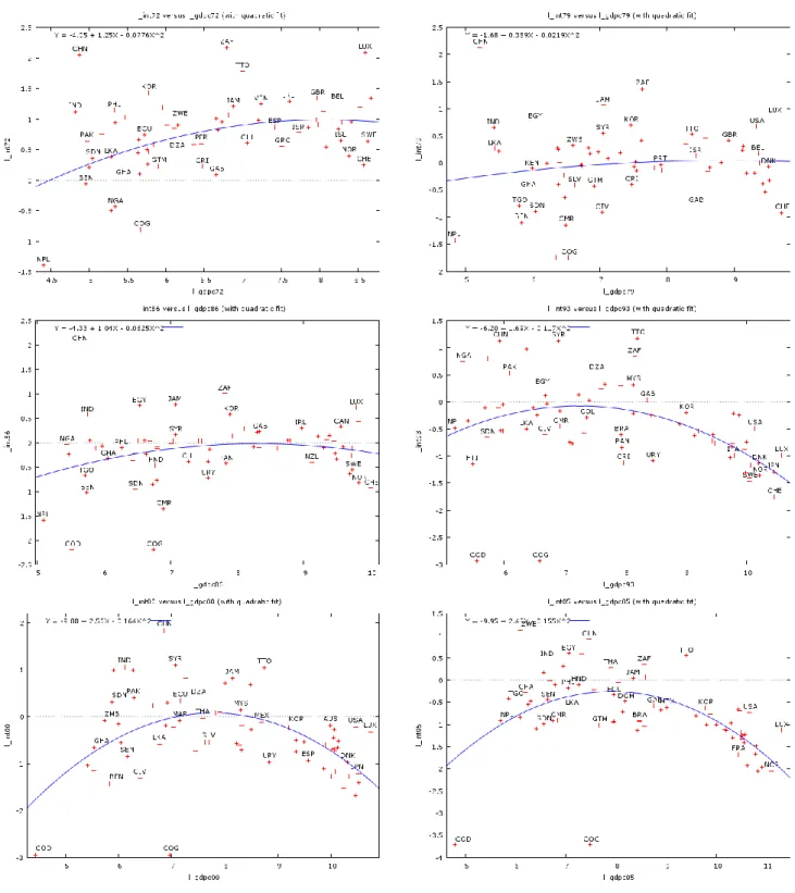
As can be seen in Figure 4, our results for GDPc are similar to Roberts and Grimes in the geo-metric progression of the curves; although this figure utilizes the Stern functional form and a different sample. The relationship is mostly linear in year 1972 but as time progresses, the relationship becomes more and more parabolic, suggesting the EKC effect is actually intensifying as time goes by.

The exclusion of extreme observation such as Nepal and the DR of Congo do not substantially modify the estimated turning point nor the geometric dispositions of the curves and thus they were left in the regression.

Worth noting is the gradual decrease in the turning point intensity which starts at approximately 2.7 tonnes of CO2 in 1972 and finishes at ~0.78 tonnes of C02 in 2005. Also interesting is that the per

capita income level at which the decrease begins has remained relatively constant throughout the pe-riod at around $2700.

21 Figure 4 - Sample cross sections for GDPc

The emergence of EKC might be a result of improving technologies that increase the efficien-cy of industrial activities which is the original proposition of the EKC.The analysis for the four in-come groups indicates that generally the CO2 emissions are being reduced but they do not form an

EKC and we can not say at what pace for each and every country this occurs.This means that even though the general trend is towards improving efficiency some countries are still on the upward going side of the Kuznets curve.

22

We are aware of the fact that some studies have reached controversial results so maybe another reason for our results is the particular sample of countries and time range that we have chosen.It is al-so possible that the quality of the data has improved over the years,especially having in mind that until recently CO2 was considered harmeless and therefore did not raise much attention, and now more

credible results may be obtained.

5.3

Fossil Fuels share

The p-values for the fossil fuel regression show a significant linear relationship from 1972 until 1987 (Appendix 3,Table 5 and Figure 8). At that point the significance level begins to fluctuate al-though it remains under the 10 % line. Since 1988 neither of the parameters have been significant. This suggests that the relationship has broken down as other factors intervene. When viewing the re-sults for the Stern method, they are not significant. This is probably due to the fact that a quadratic form simply does not reflect the relationship between fossil fuel combustion and rates of carbon in-tensity. Intuitively, carbon intensity should increase with the percentage of fossil fuel combustion. However, the results suggest that one does not determine the other.

5.4

Alternative and Nuclear Energy share

The approach by Roberts & Grimes shows significant parameters for the later part of our sam-ple (Appendix 3,Table 6 and Figure 9) .The parameters are significant since 1985 and their magnitudes yield a negative linear relationship as expected. The Stern regression is for all practical reasons insigni-ficant throughout. An interesting observation is the way the linear parameters for fossil fuels in the Roberts & Grimesregressions are significant until 1987, point at which the parameters for alternative energy sources become, and stay significant for the remainder of the period. This might suggest that alternative energy sources are becoming more relevant in defining the carbon emissions intensity of the world’s economies. This effect is not present with the Stern functional form.

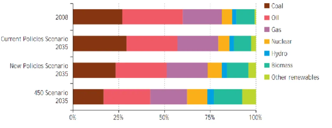
Since there is some criticism of Roberts & Grimes functional form (Mcnaughton & Lee, 1998) and since the adjusted R squared are already very low, it does not seem like there is a substantial rela-tionship between the variables. If we consider that current projections estimate a 6% of global elec-tricity will come from alternative energy, coupled with the weak relationship during the past decades, it seems as if alternative energy will not exert a large effect on world carbon intensity. As shown in Error! Reference source not found. (OECD/IEA 2010), even with optimistic projections, fossil fu-els will remain the dominant source of energy for the next decades.

23

5.5

Life Expectancy at birth

Both parameters are consistently significant at the 10% level until 1979 (Appendix 3,Table 7 and Figure 10) for both Stern and Timmons Roberts and Grimes’ regressions. In Roberts and Grimes results when compared to the linear parameter, the quadratic parameter is negligible (equals 0 throughout) which results in a linear relationship between life expectancy and carbon intensity. What’s more, the standard error is very high and increases over time. Thus, there is not a Kuznets relation-ship between the variables. To further weaken the prospect of an EKC for life expectancy, the ad-justed R squared drifts from 0.41 in 1972 to 0.12 by 2005 which mimics the results obtained by Ro-berts and Grimes.

Stern’s results show that both linear and quadratic parameters are high,therefore when plotted life expectancy exhibits a parabolic shape but at the same time the standard error is much higher (from 20.25 to 44.6) and therefore the goodness-of-fit is doubtful.

According to a survey conducted in the USA (Gogklany 2010),during the last century the country has witnessed vigorous development . To give a few examples, income, population, chemical and metal use all have increased dramatically. Of course, this has led to increased levels of CO2

emis-sions as well. One would suggest that health and longevity decrease as a result of pollution. Contrary to popular belief, the statistics prove this notion wrong. Life span has not only increased during the last decades but also the rate of disability has decreased and some of the most serious diseases occur later in life than they used to. From this overview, one can conclude that life expectancy seems to be-come less and less related to emissions, which may be the reason for the loss of explanatory power presented in the results of the above regressions. Examining the countries constituting our sample, we reached similar conclusions. The high income group (to which USA also belongs) is characterized by a steady increase in GDP per capita and life span (Appendix 4, Figure 12 & 13). The C02 emissions

are currently being reduced by the majority of the countries. However, it is worth noting that throughout the 20th _{century pollution greatly increased but still it did not have negative effects on}

lon-gevity and health. In the upper middle income group, the majority of the countries in the sample in-crease their emissions (exceptions are Dominican Republic, Jamaica,Venezuela,South Africa; Appen-dix 4, Figure 14) .The life expectancy increases for the group despite the negative externalities of pol-lution. In the lower middle income group, we observe the same trend. China is one of the largest emitters of CO2, GDP per capita rises annually at a fast pace but at the same time life span increases

as well (Appendix 4, Figure 15). In the low income group only Zambia reduces the amount of CO2

emitted every year. Again for the whole group the life span is on the rise (Appendix 4, Figure 16)

5.6

Percentage of Rural population

Neither the linear, nor the quadratic coefficient shows a significant relationship with carbon in-tensity (Appendix 3, Table 8 and Figure 11). What’s more, the adjusted R squared is seldom above 0.1. Our evidence suggests that carbon intensity is not a quadratic or linear function of the percentage of rural population. This can be partly attributed to other factors. For example, Trinidad and Tobago has rich oil resources, a sector which produces 40% of GDP but only 5% of employment while the rural population percentage has remained around 90% for the past decades (World Bank). Another example is Togo where 65% of the labor force is engaged in agriculture (Central Intelligence Agency 2011) but at the same time one of the country’s most important activities is the manufacturing and export of cement (1.2 million tons annually) which requires huge amounts of fossil fuels (Van Straaten 2002).

24

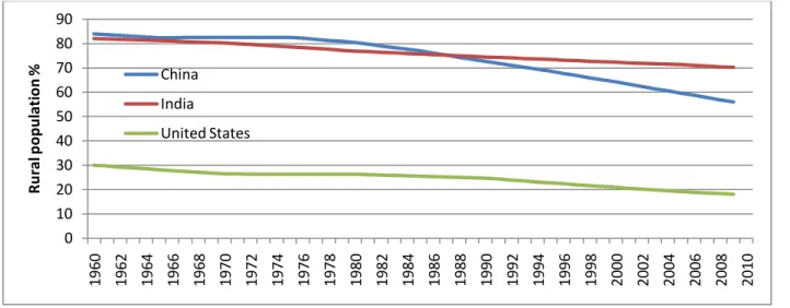
If we look at wealthy countries such as the United States we also find evidence that supports the lack of significant results in the regressions. The US has 17 % rural population. It is the world’s biggest consumer of oil, natural gas and electricity (CIA Factbook) (Figure 6 & 7 and Appendix 5, Figure 17). While India has a 70% rural population, the country ranks number 3rd in coal consump-tion, 5th in world oil consumpconsump-tion, 16th in natural gas consumption (2009 est.) and is the second larg-est producer of cement in the world (2008). It also spends around 6% of GDP on oil and gas imports (OECD/IEA 2010). Interesting characteristics that go against the EKC are exhibited by China, as well. Its rural population is 53% (2010) but it is by far the world biggest producer of cement .The country ranks 3rd _{in the world in oil consumption and 9}th _{in natural gas consumption (United States}

Geological Survey 2008).It is also the world’s second producer and consumer of electricity (CIA Factbook ).China is the largest consumer of coal worldwide (British Petroleum 2010).

Figure 6 - Rural population percentage

Figure 7 - Primary energy consumption 0 10 20 30 40 50 60 70 80 90 1960 1962 1964 1966 1968 1970 1972 1974 1976 1978 1980 1982 1984 1986 1988 1990 1992 1994 1996 1998 2000 2002 2004 2006 2008 2010 R u ra l p o p u la ti o n % China India United States 0.0 1000.0 2000.0 3000.0 4000.0 5000.0 6000.0 1965 1967 1969 1971 1973 1975 1977 1979 1981 1983 1985 1987 1989 1991 1993 1995 1997 1999 2001 2003 2005 2007 2009 Mi lli o n to nnes o il equi val ent India China US

25

5.7

Comparison of the results obtained by the two functional forms

The results yielded by both Roberts and Grimes and Stern’s econometric models support the exis-tence of EKC for GDPc.Therefore,it was proven that over time and for this specific sample of coun-tries production efficiency improves and CO2 emission intensity decreases.

Fossil fuels

Roberts and Grimes functional form led to the conclusion that for the first halv of the period fossil fuels combustion is significant and the relationship is linear.However,for the later part of the period the connection breaks down.Stern’s approach does not yield significant results throughout.

Alternative and Nuclear Energy

The results obtained by utilizing Roberts and Grimes functional form indicate that alternative and nuclear energy becomes significant at the alter part of the period,approximately at the time when fos-sil fuels lose their explanatory power.The results from Stern’s regressions are insignificant.

Life expectancy at birth

The results for life expectancy at birth are very similar for both functional forms and they show that this variable is significant throughout the period.Even though a connection between CO2 emission

in-tensity and Life expectancy is evident the correlation is linear since the quadratic parameters are low for both regressions(0 for Roberts and Grimes) and the standard errors are high.

Rural Population

Both Roberts and Grimes and Sterns regressions yielded results according to which rural population is insignificant and cannot account for CO₂ emission intensity.

26

6.Conclusion

This paper was meant to study whether the chosen variables have any relationship with regard to carbon emission intensity, if they follow the inverted U-shape curve proposed by Kuznets and how they vary in different income groups. For that purpose yearly cross-sectional regressions were run. Since previous research has not decided upon a certain econometric method, a comparison between two models was carried out. The obtained results do not differ greatly from each other. Both Stern and Roberts and Grimmes approaches indicate a connection between GDP per capita and life expec-tancy at birth to carbon emission intensity. However, the latter has a relationship to carbon emission intensity but it does not form an EKC. Following Timmons approach, we conclud that a gradual change in explanatory power from fossil fuels towards alternative and nuclear energy is present. How-ever, Stern’s approach does not yield any significant results. The results from both methods indicate that the share of rural population is insignificant with regard to carbon emission intensity.

The comparison of the two functional form led us to the conclusion that they do not yield very different results (with exception of fossil fuels and alternative and nuclear energy).Both of them may be considered credible and the results obtained by the two robust.However,the results obtained by Stern (2004) approach are more in line with current trends and therefore probably more reliable.

Our study has allowed for a broader look at the function of development indicators for the EKC. It might be of interest to future researches to study the development of the EKC not from an administrative classification, as we did but one which focuses on economic areas or trade blocks. The EKC might also have interesting results if studied by sectors or within specific classifications such as low income countries.

27

7. References

Alternative Energy Institute, Alternative Energy. Available at: http://www.altenergy.org/ [Ac-cessed May 27, 2011].

Barrett, S. & Graddy, K., 2000. Freedom, growth, and the environment. Environment and

Devel-opment Economics, 5(4), pp.433-456.

Bo, S., 2011. A Literature Survey on Environmental Kuznets Curve. Energy Procedia, 5, pp.1322-1325.

Boyce, J.K., 1994. Inequality as a cause of environmental degradation. Ecological Economics, 11(3), p.169–178.

Bradford, D.F., Schlieckert, R. & Shore, S.H., 2000. The Environmental Kuznets Curve: Explor-ing A Fresh Specification. National Bureau of Economic Research WorkExplor-ing Paper Series, No. 8001.

Brakman, S., 2009. The new introduction to geographical economics New ed., Cambridge UK ;New York: Cambridge University Press.

British Petroleum, 2010. BP Statistical Review of World Energy June 2010,

Brock, W.A. & Taylor, M.S., 2004. Economic Growth and the Environment : A Review of Theory and. Epa Publications, (1992).

Central Intelligence Agency, 2011. Togo. The World Factbook. Available at:

https://www.cia.gov/library/publications/the-world-factbook/geos/to.html# [Accessed June 5, 2011].

Clement, M. & Meunie, A., 2010. Is Inequality Harmful for the Environment? An Empirical Analysis Applied to Developing and Transition Countries. Review of Social Economy, 68(4), pp.413-445.

Cole, M.A., RAYNER, A.J. & BATES, J.M., 1997. The environmental Kuznets curve: an empiri-cal analysis. Environment and Development Economics, 2(4), pp.401-416.

Conference Board of Canada, Life Expectancy. Available at:

http://www.conferenceboard.ca/hcp/details/health/life-expectancy.aspx [Accessed May 27, 2011].

de Bruyn, S., 1998. Economic growth and emissions: reconsidering the empirical basis of envi-ronmental Kuznets curves. Ecological Economics, 25(2), pp.161-175.

Dietz, T. & Rosa, A.E., 1997. Effects of population and affluence on CO2 emissions. … of the

Na-tional Academy of Sciences of …, 94, pp.175-179.

Ehrhardt-Martinez, K., Crenshaw, E.M. & Jenkins, J.C., 2002. Deforestation and the Environmen-tal Kuznets Curve: A Cross-National Investigation of Intervening Mechanisms. Social

Science Quarterly, 83(1), pp.226-243.

Esmaeili, A. & Abdollahzadeh, N., 2009. Oil exploitation and the environmental Kuznets curve.

Energy Policy, 37(1), pp.371-374.

Gogklany, I., 2010. Population, Consumption, Carbon Emissions, and Human Well-Being in the Age of Industrialization (Part III — Have Higher US Population, Consumption, and Newer Technologies Reduced Well-Being?). Masterresource. Available at:

http://www.masterresource.org/2010/04/population-consumption-carbon-emissions-and- human-well-being-in-the-age-of-industrialization-part-iii-have-higher-us-population-consumption-and-newer-technologies-reduced-well-being/ [Accessed June 14, 2011].

28

Grossman, G.M. & Krueger, A.B., 1991. Environmental Impacts of a North American Free Trade Agreement. National Bureau of Economic Research Working Paper Series, No. 3914. Grossman, G.M. & Krueger, A.B., 1995. Economic Growth and the Environment. The Quarterly

Journal of Economics, 110(2), p.353.

Henriquez A., S., 2008. The Importance of Nuclear Energy in the Global Economy. Power, (Janu-ary).

Hettige, H., Lucas, R.E.B. & Wheeler, D., 1992. The toxic intensity of industrial production: Global patterns, trends, and trade policy. The American Economic Review, 82(2), p.478–481. Ingram, S., 2005. The Chernobyl Nuclear Disaster illustrate. M. Levine, ed., New York: Infobase

Publishing.

IPCC, 2007. Summary for Policymakers. In Climate Change 2007: The Physical Science Basis. Cambridge, United Kingdom and New York, NY, USA. Cambridge University Press. Iwata, H., Okada, K. & Samreth, S., 2010. Empirical study on the environmental Kuznets curve

for CO2 in France: The role of nuclear energy. Energy Policy, 38(8), pp.4057-4063. Kuznets, S., 1955. Economic growth and income inequality. The American Economic Review,

45(1), p.1–28.

Leitão, A., 2010. Corruption and the environmental Kuznets Curve: Empirical evidence for sulfur.

Ecological Economics, 69(11), pp.2191-2201.

Levinson, A., 2008. environmental Kuznets curve BT - The New Palgrave Dictionary of Econom-ics. In S. N. Durlauf & L. E. Blume, eds. Basingstoke: Palgrave Macmillan.

Lindmark, M., 2004. Patterns of historical CO2 intensity transitions among high and low-income countries*1. Explorations in Economic History, 41(4), pp.426-447.

Lorentzen, P., McMillan, J. & Wacziarg, R., 2008. Death and development. Journal of Economic

Growth, 13(2), pp.81-124.

Magnani, E., 2000. The Environmental Kuznets Curve, environmental protection policy and in-come distribution. Ecological Economics, 32(3), pp.431-443.

Mcnaughton, D. & Lee, T.-C., 1998. Carbon intensity and economic development 1961–1991: A comment on Roberts and Grimes. World Development, 26(12), pp.2219-2220.

Miah, M. et al., 2011a. A review of the environmental Kuznets curve hypothesis for deforestation policy in Bangladesh. iForest - Biogeosciences and Forestry, 4(1), pp.16-24.

Miah, M. et al., 2011b. A review of the environmental Kuznets curve hypothesis for deforestation policy in Bangladesh. iForest - Biogeosciences and Forestry, 4(1), pp.16-24.

Nuclear Energy Institute, Nuclear Energy Institute - Bill Gates Rides the Nuclear Wave. Available at: http://www.nei.org/resourcesandstats/publicationsandmedia/insight/march-2010/bill-gates-rides-the-nuclear-wave/ [Accessed June 3, 2011].

Nuclear Information and Resource Service, 2011. Background Information on Climate Change and Nuclear Power.

OECD/IEA, 2010. World Energy Outlook 2010, Paris: OECD Publishing.

Panayotou, T., 1997. Demystifying the environmental Kuznets curve: turning a black box into a policy tool. Environment and Development Economics, 2(4), pp.465-484.

Raupach, M.R. et al., 2007. Global and regional drivers of accelerating CO2 emissions.

Proceed-ings of the National Academy of Sciences of the United States of America, 104(24),