1985 riprap tests in flood control channels

prepared for

U. S. Army Corps of Engineers Waterways Experiment Station

Vicksburg, Mississippi BY: James F. Ruff Alaeddin Shaikh Steven R. Abt E. V. Richardson

Civil Engineering Department Engineering Research Center

Colorado State University Fort Collins, Colorado

August, 1985

FORWARD

This study was performed under a contract titled "Stability Tests of Riprap in F load Control Channels" between the U. S. Army Corps of Engineers, Waterways Experiment Station, Vicksburg, Mississippi, and Colorado State University. This report includes the tabluated and mapped data collected during the study, as well as analysis of the major results. The study plan and program was coordinated between WES and CSU by Mr. Stephen T. Maynard of WES.

Forward

.

Table of Contents

List of Tables

List of Figures

CHAPTER 1 - INTRODUCTION

Background

CHAPTER 2 - EXPERIMENTAL PROGRAM

. . . .

Experimental Setup

. . . .

Material

. . . •

. . . .

Testing Procedure and Data Collection Program

ii

iii

iv

vi

1 1 4 4 5 6

CHAPTER 3 - DATA ANALYSIS

. . . • . . . .

. • .

9

Calculation of Bed Shields' Coefficient Using Manning's

Roughness Factor For Riprap Surface • . . . .

10

Calculation of Bed Critical Shields' Coefficient Using

Darcy-Weisbach Friction Factor for Riprap Surface

21

Calculation of Bed Critical Shields Coefficient Using

Velocity Distribution Equation

. . . .

23

Comparison of the Values of Critical Shields' Coefficient

Calculated by the Previous Three Methods

. . . 29

Effect of Flat Rocks

. . . .

29

Effect of the Riprap Thickness on Bed Critical

Shields' Coefficient

. . . .

31

Effect of Riprap Gradation on Critical Shields'

Coefficient . . . • .

33

Comparison with Shields' Diagram

. . . • .

35

Maximum Stable Slopes at the Incipient Failure Runs

36

CHAPTER 4 - SUMMARY, CONCLUSIONS AND RECOMMENDATIONS

40

REFERENCES

APPENDICES

Appendix A - Sunrnary of the Test Conducted

Appendix B - Velocity Data

Appendix C - Velocity Profiles

iii

42

TABLE 2.1 2.2 3.1 3.2 3.3 3.4

3.5

3.6 3.7 3.8 3.9 3.10 LIST OF TABLES DESCRIPTION Values of the D Id of the riprap material

'bl

lefff5 Study and the 1982 and 1983 Reports

Methods of Testing

Calculation of Manning's and Shields' Coefficients for Riprap of d

=

1 in.

50

and Thickness = 2 in.

Calculation of Manning's and Shields' Coefficients for Riprap of d = 1 in.

50

and Thickness= 2 in. (after removing rocks).

Calculation of Manning's and Shields' Coefficients for Riprap of d = l in. and Thickness = 3 in. 50

Calculation of Manning's and Shields' Coefficients for Riprap of d = 2 in. and Thickness = 4 in. 50

Calculation of Manning's and Shields' Coefficients for Riprap of d = 2 in.

50

and Thickness = 6 in.

Values of Bed Manning's Roughness Factor Calculated From Experimental Data and Equations Listed

Calculation of Bed Critical Shields' Coefficient Using Darcy-Weisbach Friction Factor

Calculation of Bed Critical Shields' Coefficient Using Velocity Distribution Equation

Calculation of Bed Critical Shields' Coefficient Using Velocity Distribution Equation

Values of Bed Critical Shields'

Coefficients Calculated by Three Different Methods Listed

iv

PAGE 5 6 15 16 17 18 19 20 22 26

27

28

3.11 Values of d ₅₀ ID and F roude Number 30 3.12 Values of C and k for Some Selected 33

CV S

Runs Calculated Based on "General and Local" Datums

3.13 _{Values of C and R* c} 37

LIST OF FIGURES

FIGURE DESCRIPTION PAGE

l. l Design Gradation of Riprap Material of This Study (l 985) and the 1982 and 1983

Reports. 3

2.1 Gradation of Rip rap Material Tested 8

3. l Values of Overall Critical Shields' Coefficient for Different Rock Sizes

and Thicknesses 32

3.2 Variation of Overall Critical Shields'

Coefficients With Riprap Gradation 34

3.3 l he Shields' Diagram 38

3.4 Maximum Stable Slope vs. Discharge 39

INTRODUCTION

1.1 §ackground

This study is a continuation of the work to determine the point of incipient failure and other hydraulic characteristics of riprap for providing criteria for design of stable ripraps in flood control channels. The study initiated in l 981 at Colorado State University (CSU) by and in cooperation with the U. S. Army Corps of Engineers, Waterways Experiment Station (WES), Vicksburg, Mississippi. The previous work was presented in two reports. The first report entitled, "St.ability Tests of Riprap in Flood Control Channels," was prepared by A. A. Fiuzat, Y. H. Chen and 0. B. Simons in October, 1982, and is referred to as the "1982 Report" throughout this latest report (1985). The second report was entitled, "Supplemental Stability Tests of Riprap in Flood Control Channels" and was prepared by A. A. Fiuzat and E. V. Richardson in December, 1983. The second report similarly is referred to as the "198 3 Report" throughout this new report (198 5 ). The equipment, flume test procedures, and data collection methods are either identical or similar to those procedures described in the 1982 and 1983 Reports.

Two sizes riprap materials were tested. One material had a d ₅₀

=

1.0 in. and the other had a d

=

2.0 in. Both riprap sizes had the E TL 1110-2-120 gradation

50

2

shown in Figure l. l. The design gradation of the riprap material of the 1982 and

1983 Reports is also shown in this Figure. Tests were performed for both size

gradations with the thickness of the riprap set at 2d and then at Jd . The failure

_{50 50}

criterion for both riprap thicknesses was the exposure of the underlying filter

blanket observed after a run. Incipient failure was then defined as the run when the

flume slope was set one increment lower than the failure run. In the following

chapters the experimental program and analysis of data are presented.

a::

w

z

LL

.__

z

w

(.)

a::

w

a.

801-

GRADATION ETL

1110-2-120---8

1985

STUDY

I

60

I v

40

I

GRADATION OF

1982

a

1983---REPORTS

I

20

o.._ ________

_0.1

____.so-~---.---~---

_0.2

_0.3

0.4

0.6

d I dso

0.8 1.0

2.0

Fiqure 1.1 Gradation of rinrap material of this study (1985) and the 1982 and 1983 Reports.

4

CHAPTER 2

EXPERIMENT AL PROGRAM

The experimental program conducted for this phase of the riprap study

generally follows the procedures and methods described in the l

982

and

1983

Reports.

In this chapter the materials and methods that differ from those of the

1982

and 1983 Reports are explained. Those which are not explained are similar to the

1982

and

1983

Reports ..

2 .. l Experimental Setup

For the first 18 runs, the test section was 50 ft long with a transition section of

40 ft. From the upstream end of the flume (Station 0) to the beginning of the

transition section (Station 60), rocks of 6 to l 0 in .. in diameter were cemented to the

flume floor. The 40

ft

transition section (from Station 60 to station 100) was made

of l in. rocks cemented to the flume floor. For the remaining runs (from run

1119

to

94), the test section was reduced to 40

ft

and the transition section was constructed

by placing rocks of similar size as the test section in the transition. These rocks in

the transition section were not cemented to the flume floor; instead they were

covered with a wire mesh (chicken wire) to hold them in place. The transition

section was 40 ft long and started at Station 70. The test section started at Station

l l 0.. The rocks in the transition section were placed such that the top of the rocks

in the test and transition sections were in the same plane for all riprap thicknesses.

The first 70 ft of the flume was comprised of 6 to 10 in. rocks cemented on the floor.

d ₅₀

=

l in. rocks was 2.68 and the d ₅₀ = 2 in. rocks was 2.64. The gradations of the riprap material tested are shown in Figure 2. l. The gradation of d

50

=

l in. riprap

was determined using a mechanical sieve shaker. The gradation of d

=

2 in. riprap

so

was established using flat sieves manufactured at CSU for this purpose. The values

of d /d _{95 15} of the riprap material are presented in Table 2. l. In this Table the

values of d /d of the riprap material of the 1982 Report (for d

=

1 in) and the

95 15 so

l 983 Report (for d

=

2 in) are also presented.

50

l able 2.1 Values of the d /d of the riprap material of this (1985) Study and _{85 15} the 1982 and 1983 Reports.

1 his Study ( 1985) 1982 Report 1983 Report

d (in) 2 l.87

so

d /d (in)

SS l.5 2.0

2.4

2.8

4.4

For the first series of tests (d ::: l in., runs ti 1- 31) the riprap material

50

consisted of about 10 percent (by weight) flat rocks. The flat rocks were removed the first series of tests. For the rest of the runs, the riprap material met the ;hape criteria of the Army Corps of Engineers. These criteria (C.O.E. Report

-E.m l l l0-2-1601, 1970) are:

1. The stone shall be predominately angular in shape.

2. No more than 25 percent of the stones reasonably well distributed throughout the gradation shall have a length more than 2.5 times the breadth or thickness.

6

2. 3 Testing Procedure and Data Collection Proqram

The data collected included bed and water surface elevations, discharge, velocity profiles using either a pitot-static tube or an Ott meter, and the size and location of areas washed free of riprap down to the underlying filter cloth. Trials were performed with riprap thickness of 2d and 3d . _{so so}

A "general datum" for each rock thickness was established by the following procedures:

( l) The flume was set to the horizontal position.

(2) Water was added to the flume until about 90% of the rocks were covered

with water.

(3) The elevation of the water surface was measured along the flume at I 0 ft intervals; at the locations where flow depths were measured.

(4) These elevations were considered as the elevations of the bottom of channel (general datum) in measuring the flow depth.

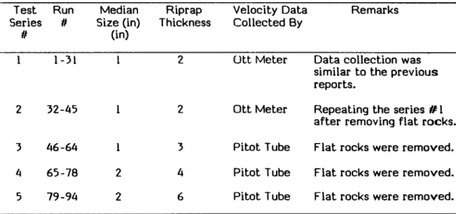
Five series of tests with a total of 94 runs were performed. The methods of testing are summarized in Table 2.2. Other information such as bed slope, water temperature, area washed, and test duration for each run are presented in Appendix A. Test Run Series II II 2 3 4 5 1-31 32-45 46-64 65-78 79-94 Median Size (in) (in) 2 2

Table 2.2 Methods of Testing Rip rap Thickness 2 2 3 4 6 Velocity Data Collected By Ott Meter Ott Meter Pitot Tube Pitot Tube Pitot Tube Remarks

Data collection was similar to the previous reports.

Repeating the series 11 l after removing flat rocks. Flat rocks were removed. Flat rocks were removed. Flat rocks were removed.

As shown in Table 2.2, the test procedure for the riprap of d

_so

=

1 in. and

thickness

=

2 in. was similar to that of the 1982 and 1983 Reports. For test series

No. 3 to 5, a pi tot tube was used to measure the velocities. For these last series of

tests the velocity data were collected at 0.05, 0.10, 0.15, 0.2, 0.3, 0.4, 0.5, 0.7, 0.90

above the "general datum." In addition, the pitot tube was set on the top of the

rocks and velocities at these points also were measured. These points established by

the pi tot tube on top of the rocks will be referred as the "local datums." The

elevations of these local datums in most cases were below the general datum. For

the last 3 series of tests the comprehensive velocity data were collected for every

test, and not only for the incipient failure conditions. Velocity profile traverses

were taken at several locations in the cross sections throughout the test section.

Specific locations are listed for each run in Appendix B.

0 0 <] Q. 0

..

a.

a:

c

0

Q. 0

..

a.

·-a:

c C\I <] 0 CX> 0 U) 8 0

v

~

3N1.:1

lN3~~3d 0 N 0 C\I 0 U)

0

v

0

ro

0

N

d

0 tO "O ... "O

CHAPTER 3

DAT A ANALYSIS

The failure criterion for the riprap stability study was the exposure of the

underlying filter blanket after a run. For a given discharge, the run at which the

flume slope was one increment lower than the failure run was regarded as the

incipient failure run. In this study the term "incipient failure" was used in place of

"incipient motion" to avoid confusion. Incipient motion condition is considered to

occur when the exerted force by flow just overcomes the resistance force of a

particle to motion without moving the particle. However, at the incipient failure

condition, a substantial amount of riprap material may move without exposing the

underlying filter blanket. The latter condition can occur specially at greater

thicknesses of ripraps.

In this study there were some exceptional cases where the above criterion was

not met. These cases are explained in the following.

The transition section for the first 18 runs was made of 1 in. rocks cemented to

the flume floor, as previously mentioned. The transition section was 40 ft. long; the

elevation of upstream end was 8 in. above the elevation of downstream end with a

slope of 1.7 percent relative to the flume floor. The flow accelerated down this

slope and did not produce a smooth transition into the test section. Because of this

transition section, it was not possible to reach uniform flow depth within the test

reach at discharge greater than 25 cfs, and all riprap failure occurred at the

beginning of the test section due to high velocity of flow. The test result was not

considered to be representative of behavior of the riprap under uniform flow for

flows greater than 25 cfs because of the problems caused by the transition section.

10

Therefore, the transition section was reconstructed and the tests were repeated. Since the above problems were not pronounced for the flow rate of 25 cfs, the tests were not repeated for the 25 cfs flow rate. The data for runs 8 to 18 were not used for analysis in this chapter, however, they are presented in Appendices.

In run numbers 27, 37, 41 and 45 the failure occured at the beginning of the test section and was believed to be the result of local disturbances at the junction between the transition and test section. These runs were not considered to be the failure runs but the incipient failure runs. The washed area for these runs was less than three square feet which occurred at the beginning of the test section.

For run 1111 (d = 2 in, 2d thick riprap) failure was not observed when the

50 50

flow rate was 25 cfs and flume was at its maximum slope (about 1.9 percent). When the riprap thickness was increased to Jd , failure did not occur at flows equal to or

50

less than 50 cfs and maximum flume slope (run lls 80 and 84). Run 1184 was, however, considered to be the incipient failure run since some of the rocks were moved and several dips were observed on the riprap surface.

The following methods are used to calculate the bed Shields' coefficients from the collected data.

l) Using Manning's roughness factor for riprap surface 2) Using Darcy-Weisbach friction factor for rip rap surface J) Using velocity distribution equation

J. l Calculation of Bed Shields' Coefficient Using Manning's Roughness Factor For Riprap Surface

The development of the equations to calculate the Manning's roughness factor for the riprap surface nb is presented in the 1982 Report (p. 19). This method is a side-wall correction technique (Vanoni, 1975, P. 152) which can be used to calculate

the average shear stress on the bed, i:b, and bed Shield's coefficient Cb. The

assumptions in this technique are: a) the flow cross-sectional area can be divided

into two parts, Ab and Aw where resistance to flow is caused by the bed and the

walls respectively, and b) the mean velocity and energy gradient are the same for

Ab and Aw and Manning's equation can be applied to each part of the cross-section

as well as to the whole. The resulting equations (developed in the 1982 Report) for

this technique are:

where

l.49 R'/, S 1/z n

=

V

R w =

_n

_3/2 w (3.1) (3.2) (3.3)

n,nb,nw

=

Manning's roughness factor for the flume (overall), bed, and

v

s

p

Pb

PW

R

Rb

Rw

w

0

=

=

=

=

=

= =

=

=

=

wall respectively

average velocity of flow in fps

channel slope in ft/ft

wetted perimeter of channel

=

w + 20, in ft

wetted perimeter for bed

=

w, in ft

wetted perimeter for walls

=

20, in ft

hydraulic radius of channel

=

A/p

=

w0/(w+20), in ft

hydraulic radius for bed

=

Ab/pb, in ft

hydraulic radius for walls= Aw/pw' in ft

channel width

=

8 ft

12

Substituting the values of pb

=

w

=

8 ft, P

_w

=

20, and n

_w

=

0.012

(for smooth painted

wall and plexiglas, Chow,

1959,

p.

110 -111)

in equation

cs.

3)

results in

(3.4)

The value of nb calculated from equation

(3.4)

can be used to calculate the vlaues of

the average shear stress on bed and the bed Shields' coefficient. The calculation

procedure is as follows:

1.

Calculate n from equation

(3 .. 1)

for known values of

V,

R, and S.

2.

Calculate nb from equation

(3.4).

3.

Calculate Rb from equations

(3.2)

for known values of Rand n.

4.

Calculate average shear stress on bed using the relationship

Tb= Yw

Rb 5

(3.5)

where

y

w

is the unit weight of water.

5.

Calculate Cb using the relaionship

(s-1) d _so

(3.6)

where

Ys

is the specific weight of rock, s is the specific gravity of rocks

(Y/Yw),

and d is median size of the riprap in

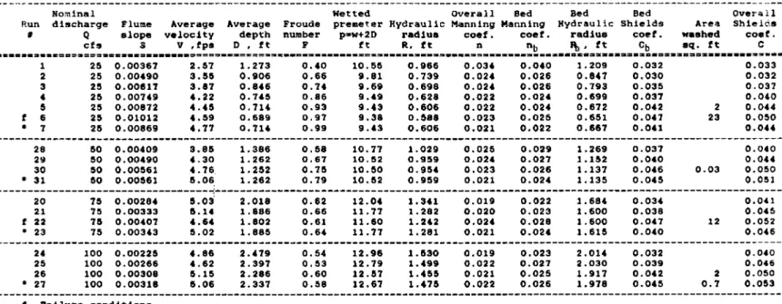
_so ft.

The values of n, nb, and Cb are calculated by the above procedure and results

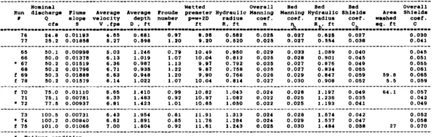
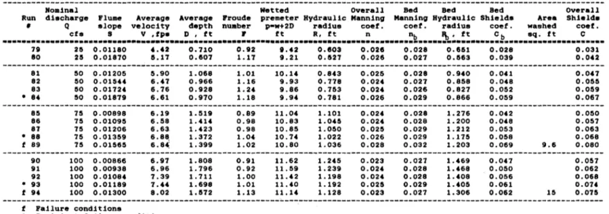
are presented in Tables 3.1 to 3.5. The values of bed Shield's coefficitml. for

incipient failure runs will be termed the bed critical Shields' coefficient; the bed

critical Shields' coefficient calculated by this method (using Manning's roughness

factor) will be denoted by ccn·

In addition of the bed Shield's coefficient, the values of the overall Shields' coefficient C, are also calculated and presented in Table 3.1 to 3.5. The overall Shields' coefficient is defined as:

C

=

OS

(s - l} d₅₀ (3.7)

The values of C for incipient failure runs will be termed the overall critical Shields' coefficient and will be denoted by C . _c

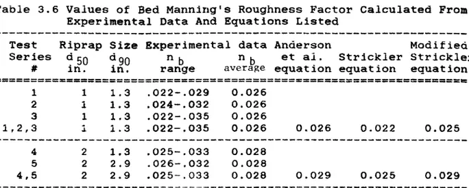
The range and average values of the bed Manning's roughness factor, for the five series of tests, are summarized in Table 3.6. This Table also contains the values of Manning's roughness factor calculated by the two following equations:

1. Anderson et al. ( 1970} equation

n

=

0.0395 d ₅₀ where d is in feet, and

50

2. Strickler's equation (Simons and Senturk, 1977, p. 309}

n = d ₉₀ 116 /26

wtu~re d is in meters.

90

(3.8}

The results in Table 3.6 show that l} the values of n obtained by Anderson et al. equation are in agreement with the values of nb obtained experimentally; and 2} Strickler's equation underestimates the bed Manning's roughness factor.

14

The coefficient of Strickler's equation was modified in order to fit the data. The modified equation is:

n = d 116 _{/22.4 (d in meters)}

90 90 (3.10)

The coefficient 1/22.4 was obtained by calculating the corresponding coefficient of Strickler's equation for each nb value given in Tables 3.1 to 3.5 and then averaging all coefficients. The calculated values of n from equation (3.10) are also presented in Table 3.6.

cfs s V ,fps D , ft F ft R, ft n nb 1'> ~ ft Cb sq. ft c •=•==•2=•=========•======••••••=====••==•====•••••=•••••••==s=•••••••••••••••=••••••••=••••••••••••••=•=•••=•••••••••••••s=••• 1 25 0.0031;1 2.51 1.213 0.40 10.55 0.966 0.034 0.040 1.209 0.032 0.033 2 25 0.00490 3.55 0.906 0.66 9.81 0.739 0.024 0.026 0.841 0.030 0.032 3 25 0.00617 3.81 0.846 0.14 9.69 0.698 0.024 0.026 0.793 0.035 0.037 4 25 0.00749 4.22 0.145 0.86 9.49 0.628 0.022 0.024 0.699 0.031 0.040 5 25 0.00872 4.45 0.714 0.93 9.43 0.606 0.022 0.024 0.612 0.042 2 o.ou f 6 25 0.01012 4.59 0.689 0.91 9.38 0.588 0.023 0.025 0.651 0.047 23 0.050 • 1 25 0.00869 4.11 0.114 0.99 9.43 0.606 0.021 0.022 0.661 0.041 0.044 ---~---28 50 0.00409 3.85 1.386 0.58 10.11 1.029 0.025 0.029 1.269 0.031 0.040 29 50 0.00490 4.30 1.262 0.67 10.52 0.959 0.024 0.021 1.152 0.040 o.ou 30 150 0.00561 4.16 1.252 0.115 10.50 0.954 0.023 0.026 1.137 0.046 0.03 0.050 • 31 50 0.00561 5.0~ 1.262 0.19 10.52 0.959 0.021 0.024 1.135 0.045 0.051 ---~---_{20 75 0.00284 5.03 2.018 0.62 12.0, 1.3U 0.019 0.022 1.684 0.034 0.041} 21 75 0.00333 5.14 1.886 0.66 11.71 1.282 0.020 0.023 1.600 0.038 0.045 f 22 15 0.00407 4.64 1.802 0.61 11.60 1.242 0.024 0.028 1.600 0.047 12 0.052 • 23 75 0.00343 5.02 1.885 0.64 11.11 1. 281 0.021 0.024 1.615 0.040 0.046 24 100 0.00225 4.86 2.479 0.54 12.96 1.530 0.019 0.023 2.014 0.032 o.o,o 25 100 0.00266 4.62 2.397 0.53 12.79 1.499 0.022 0.021 2.030 0.039 0.046 26 100 0.00308 5.15 2.286 0.60 12.57 1.455 0.021 0.025 1.917 0.042 2 0.050 • 27 100 0.00318 5.06 2.337 0.58 12.67 1.475 0.022 0.026 1.918 0.045 0.7 0.053

---

_{f Failure conditions}

• Incipient failure conditions

Table 3.1. Calculation of Manning's and Shields' Coefficients For Riprap of d _so

=

l in. and Thickness

=

2 in.

~

Bo11inal Wetted Overall Bed Bed Bed overall Run discharge Pluae Average Average Proude pre11eter Hydraulic Manning Manning hydraulic Shields Area Shield• • Q •lope velocity depth nwaber p-w+2D radius coef. coef. radius coef. washed coef.

cfs s V , fP• D , ft r ft R, ft n nb Rf>·. ft Cb sq. ft c

···--·-···-···=···

33 3' 35 t 36 • 37 f 32 • 41 25 0.00998 25 0.01088 25 0.01186 25 0.01337 25 0.01204 50 0.00558 50 0.00'75 ... a; 4.51! 4.72 4.95 4.77 ... 90 4 •. 71 0.68' 0.703 0.612 0.618 0.651 1.300 1.353 0.94 0.95 1.01 1.11 1.04 0.76 0.71 9.37 9.U 9.34 9.2' 9.30 10.60 10.71 0.584 0.598 0.575 0.535 0.560 0.981 1.011 0.024 0.02' 0.024 0.023 0.023 0.022 0.022 0.025 0.026 0.025 o.ou 0.025 0.025 0.025 0.648 0.667 0.637 0.587 0.617 1.115 1.215 0.0"6 0.052 0.054 0.056 0.053 0.047 0.0'1 1.2 2.7 10.8 2.5 0.049 0.055 o.on 0.059 0.056 0.052 0.046 ---~---~--_{t 38} t 39 • 40 42 '3 t " _{• 45} 75 0.00402 75 0.00317 75 0.00345 100 0.00314 100 0.00403 100 0.00'36 100 0.00354 t Failure conditions 5.02 5.00 4.8' 4.97 4.90 5.20 5.09

• Incipient failure conditions

1.832 1.8'2 1.918 2.371 2.415 2.210 2.332 0.65 0.65 0.62 0.57 0.56 0.62 0.59 11.66 11.68 11.8' 12.14 12.83 12.'2 12.66 1.257 1.261 1.296 1.489 1.506 1.424 1.'73 0.022 0.021 0.021 0.022 0.025 0.024 0.023 0.026 0.025 0.025 0.027 0.032 0.029 0.028 1.599 1.597 1.659 2.013 2.119 1.931 1.999

Table 3.2. Calculation of Manning's and Shields' Coefficients for Riprap of d

_so

=

l in .. and

Thickness= 2 in. (after removing flat rocks).

0.046 0.043 0.041 0.045 0.061 0.060 0.051 0.4 0.1 11.1 2.5 0.053 0.050 0.047 0.0&3 0.010 0.069 0.059 -..t

°'

····--···-···-···---···

_•6 41 48 • 57 f 58 •9 50 52 f 53 f 54 f 55 • 56 25 0.00880 25 0.01011 25 0.01313 25 0.01475 25 0.01626 50 0.00526 50 0.00636 50 0.00726 50 0.00802 50 0.00732 50 0.00732 50 0.00641 ,,37 •• 61 5.02 5.02 5.52 ,,9, 5.36 5.7• 5.66 5.64 5.03 5.11 0.720 0.91 9.U 0.688 0.98 9.38 0.640 1.11 9.28 0.625 1.12 9.25 0.568 1.29 9.14 1.268 0.77 10.5• 1.169 0.87 10.34 1.096 0.97 10.19 1.095 0.95 10.19 1.111 0.94 10.22 1.245 0.79 10.49 1.231 0.81 10.'6 0.610 0.023 0.025 0.581 0.023 0.024 o.&52 0.023 0.024 0.5U 0.02.f. 0.026 0.497 0.022 0.023 0.963 0.021 0.024 0.905 0.021 0.023 0.860 0.020 0.022 0.860 0.021 0.02' 0.869 0.021 0.023 0.949 0.02.f. 0.028 0.9U 0.023 0.025 0.679 0.0'3 0.649 0.0•7 0.606 0.057 0.595 0.063 0.539 0.063 1.139 0.043 1.053 0.048 0.987 0.051 0.996 0.057 1.004 0.052 1.14' 0.060 1.118 0.052 23 37.• 2.3 3.7 o.oo 0.050 0.060 0.066 0.066 0.048 0.053 0.057 0.063 0.058 0.065 0.057

---

59 75 0.00423 4.90 1.907 0.63 11.81 1.291 0.023 0.028 1.682 0.051 0.058 • 60 75 0.00517 5.11 1.814 0.67 11.63 1.248 0.024 0.029 1.618 0.060 0.067 f 61 75 0.00621 5.50 1.714 0.74 11.'3 1.200 0.024 0.028 1.533 0.068 '9.5 0.076

---

_{62 100 0.00406 4.63 2.513 0.51 13.03 1.5'3 0.027 0.035 2.232 0.065 0.073} t 63 100 0.00'57 5.25 2.210 0.62 12 .'2 1.424 0.024 0.030 1.937 0.063 2 0.072 • 64 100 0.00409 5.10 2.298 0.59 12.60 1 . .f.60 0.024 0.030 2.002 0.058 0.067

---

f Failure conditions

• Incipient failure condition•

Table 3.3. Calculation of Manning's and Shields' Coefficients for Riprap of d

=

l in. and

50

Thickness

=

3 in.

Nominal Wetted Overall Bed Bed Bed Overall Run discharge Flume Average Average Froude premeter Hydraulic Manning Manning Hydraulic Shields Area Shields

• Q slope velocity depth number p•w+2D radius coef. coef. radius coef. washed coef.

ct• s v ,tp• D , ft r ft R, ft n n,_ R • ft c aq. ft c

···-'*···~---···u ₁₆

... .

17 u.e 0.01193 2!L2 0.01858 •• 55 5.27 0.681 0.598 0.97 1.20 t.38 9.20 O.H2 0.520 0.025 0.02& 0.027 0.027 0.&25 0.55• 0.027 0.038 0.030 0.0•1

---

_{65 50.1 0.00998 5.03 1.246 0.79 10.49 0.950 0.029 0.033 1.089 0.040 0.0'5} 66 50.0 0.01318 6.13 1.019 1.01 10.0• 0.812 0.025 0.028 0.901 0.045 0.051 • 61 50.2 0.01519 6.36 0.981 1.13 9.91 0.792 0.025 0.027 0.876 0.049 0.055 68 50.2 0.01796 6.71 0.935 1.22 9.87 0.758 0.025 0.027 0.83 .. 0.055 0.061 t 69 50.3 0.01888 6.63 0.9'8 1. 20 9.90 0.766 0.026 0.029 0.841 0.059 59.8 0.065 t 18 50.2 0.01579 6.14 1.022 1.07 10.0• 0.814 0.027 0.030 0.908 0.052 5.5 0.059

---

_{f 70} 71 • 72 13 • 1• t 75 75.0 75.1 77.5 100.5 100.2 101.0 0.01110 0.00781 0.00937 0.00731 0.00840 0.01066 t Failure condition 6.65 6.33 6.81 6.43 6.62 1.00

• Incipient failure conditions

1.UO 1.483 1.'23 1.95• 1.891 1.80• 0.99 0.92 1.01 0.81 o.85 0.92 10.82 10.97 10.85 11.91 11. 78 11.61 1.043 1.082 1.050 1.313 1.28' 1.2'3 0.024 0.022 0.022 0.024 0.02• 0.025 0.028 0.025 0.025 0.028 0.029 0.030 1.197 1.236 1.193 1.57• 1.537 1.'8 .. 0.049 0.035 0.0•1 o.ou 0.0•1 0.058

Table 3.4. Calculation of Manning's and Shields' Coefficients for Riprap of d _so

=

2 in. and Thickness = 4 in. 64.1 27 0.057 o.ou 0.049 0.052 0.058 0.010 co

···-···-···

_{79 H 0.01110 4.'2 0.110 0.92 t.'2 0.103 O.OH 0.028 0.651 0.028 0.031} 80 25 0.01870 5.17 0.607 1.1'1 9.21 0.527 0.026 0.027 0.563 0.039 0.0'2

---

81 50 0.01205 5.90 1.068 1.01 10.14 0.843 0.025 0.028 0.9'0 0.0•1 0.047 82 50 o.ouso 6.47 0.966 1.16 9.93 0.718 0.02' 0.021 0.858 0.0'8 0.055 83 50 0.0172' 6.'16 0.928 1.2' 9.86 0.753 0.02' 0.026 0.82'1 0.052 0.059 • 84 50 0.01819 6.61 0.9'10 1.18 9.9' 0.'181 0.026 0.029 0.866 0.059 0.06'1

---

85 15 0.00898 6.19 1.519 0.89 11.04 1.101 0.02' 0.028 1.276 0.0'2 0.050 86 75 0.01095 6.58 1.414 0.98 10.83 1.045 0.02' 0.028 1.200 0.0'8 0.057 81 75 0.01206 6.63 1.'23 0.98 10.85 1.050 0.025 0.029 1.212 0.053 0.063 • 88 75 0.01359 6.8~ 1.3'12 1.04 10.14 1.022 0.026 0.029 1.175 0.058 0.068 f 89 '15 0.01565 6.84; 1.399 1.02 10.80 1.036 0.028 0.032 1.203 0.069 9.6 0.080

---

90 100 0.00866 6.97 1.808 0.91 11.62 1.245 0.023 0.027 1.'69 0.047 91 100 0.00938 6.96 1.'196 0.92 11.59 1.239 0.02' 0.028 1.468 o.oso 92 100 0.0108' 7.39 1.711 1.00 11.'2 1.198 0.02' 0.028 1.•oa 0.056 • 93 100 0.01189 'l.'4 1.698 1.01 11.•0 1.192 0.025 0.029 1.405 0.061 f 9• 100 0.01300 8.02 1.n2 1.13 11.14 1.128 0.023 0.027 1.306 0.062 f Failure conditions

• Incipient failure conditions

Table 3.5. Calculation of Manning's and Shields' Coefficients for Riprap of d

=

2 in. and

50 Thickness

=

6 in .. 0.057 0.062 0.068 0.01• 15 0.015

...

ID

20

Table 3.6 Values of Bed Manning's Roughness Factor Calculated From Experimental Data And Equations Listed

Test Series

#

Riprap Size Experimental data Anderson Modified d 50 d 90 n b n b et al. Strickler Str ickle?

in. in. range avera~e equation equation equation

==================================================================

1 2 3 1,2,3 4 5 4,5 1 1 1 1 2 2 2 1.3 .022-.029 1. 3 . 024-. 032 l.3 .022-.035 1.3 .022-.035 1.3 .025-.033 2.9 .026-.032 2. 9 • 025-. 033 0.026 0.026 0.026 0.026 0.028 0.028 0.028 0.026 0.029 0.022 0.025 0.025 0.029

3.2

Calculation of Bed Critical Shields' Coefficient Using Darcv-Weisbach Friction

Factor For Riprap Surface

This method is similar to the method presented in Section

J.

l,

I.hat. is,

a

side-wall correction technique which results in average values of shear stress on bed

and bed Shields' coefficient. The only difference between these two methods is that

in section

3.1

the Manning's equation was used to describe the relationship between

resistance to

flow

and hydn-tulic parameters while in this section

thr!

Oarcy-Weisbach equation is used to describe such a relationship. The develoµrnent

of the equations for this method are presented in the 1982 Report (p. 22). The

resulting equations are:

(s-l) d ₅₀

C cf

=

Cb for incipient failure runs

where

v2

a=

gSR

f =

Rw

.ft.

-f-= f w

=

bed Shields' coefficient

=

bed critical Shield's coefficient

=

hydraulic radius for bed in ft

=

channel hydraulic radius in ft

(3.11)

(J.12)

(J.13)

(J.14)

=

Darcy-Weisbach friction factor for the flume, bed and wall

respectively

=

Reynolds number for channel and wall respectively

The calculated values of the bed critical Shields' coefficient for incipient

failure conditions (C cf) are presented in Table 3. 7.

Riprap Nominal Overall Overall Wall Bed Bed Bed median Riprap discharge Run Flume Average Average hydraulic Reynolds friction friction friction hydraulic Shields

size thickness Q # slope velocity depth radius number factor R/f factor factor radius

in. in. ofs s v, fps D, ft R, ft R f fw fb Rb

2 2 2 2 2 2 Table J.7 2 25 1 0.00869 4.77 0.714 0.606 1.16E+06 0.060 1.94E+07 0.015 0.068 0.688 0.043 2 50 31 0.00561 5.06 1.262 0.959 1.94E+06 0.054 3.59E+07 0.013 0.067 1.188 0.048 2 75 23 0.00343 5.02 1.885 1.281 2.57E+06 0.045 5.73E+07 0.012 0.060 1.720 0.042 2 100 27 0.00318 5.06 2.337 1.475 2.99E+06 0.047 6.33E+07 0.012 0.068 2.116 0.048 2 2 2 2 3 3 3 3 4 4 4 6 6 6 25 50 75 too 25 50 75 100 50 75 100 50 75 100 37 0.01204 41 0.00475 llO 0.00345 45 0.003514 57 0.01ll75 56 0.00647 60 0.00517 64 0.00409 67 O.OT519 72 0.00937 74 0.008140 811 0.01879 88 0.01359 93 0.01189 4.71 Jt.71 4.84 5.09 5.02 5 .11 5 .11 5.10 6.36 6.81 6.62 6.61 6.88 7.JJ4 0.651 1. 353 1.918 2.332 o.625 1 .231 1 .814 2.298 0.987 1.423 1 .891 0.970 1.312 1.698 0.560 1 .07E+06 1.011 1.90E+06 1.296 2.51E+06 1.ll73 3.00E+06 0.541 1.09E+06 0.941 1.92E+06 1.248 2.5SE+06 1.ll60 2.98E+06 0.792 2.01E+06 t.050 2.86E+06 1.28Jt 3.J40E+06 0.781 2.06E+06 1.022 2.81E+06 1.192 3.55E+06 0.076 1.40E+07 0.056 3.42E+07 0.049 5.lOE+07 0.052 5.78E+07 0.082 1.33E+07 0.060 3.20E+07 0.064 4.01E+07 0.059 5.04E+07 0.077 2.63E+07 0.055 5.23E+07 0.063 5.36E+07 0.086 2.39E+07 0.076 3.72E+07 0.066 5.38E+07 0.015 0.013 0.012 0.012 0.016 0.014 0.013 0.013 0.014 0.012 0.012 0.014 0.013 0.012 0.086 0.070 0.067 0.075 0.092 0.074 0.087 0.086 0.092 0.010 0.088 0.104 0.097 0.089

Calculation of Bed Critical Shields• Coefficient Using Darcy Weisbach Friction Factor

0.633 1 .271 t. 761 2.128 0.609 1 .166 1. 698 2. 121 0.952 1.338 1.112 0.939 1 .311 t .603 0.051.1 0.043 O.Oll3 0.054 0.064 0.054 0.063 0.062 0.052 0.045 0.053 0.063 0.064 0.068 N N

3. 3 Calculation Of Bed Critical Shields Coefficient Using Velocity Distribution

Equation

The Prandtl-Von Karman velocity distribution equation is used in this section to

calculate the bed critical Shields' coefficient

C • _CV

The Prandtl-Von Karman

equation is presented as (Chow,

1959,

p.

202)

where

u

u*

z

k s

30z

u =

5. 75

u* log k

=

=

=

=

s

velocity at height

z

[LIT] in ft/sec

shear velocity [L/T] in ft/sec

vertical height above the "bed" [L] in ft

equivalent roughness height

[L]

in ft

Equation

(3.15)

can be written as

or

where

30

u =

5.75

u* log

z + 5.75

u* log

k

U =a log

z

+ b

a = 5.75

u*

30 b

=

5. 75 U

*

log k s

s

(3.15) (3.16) (3.17) (3.18) (3.19)

Equation

(3.17)

indicates that if velocities are plotted versus depth on

semi-logarithmic paper the value of shear velocity, U*' can be determined from the

slope of the line passing through the data points. The value of "b" can be evaluated

by using known points on the line. The magnitude of k then can be calculated from

_s

equation

(3.19).

For a known value of u .. , the critical bed shear stress, 'tc' and

24

't _c

=

'tb for incipient failure runs 2

't _c

₌

_pU*

(3.20)

CCV ::: _{{ys- 'Yw) d} 'tc _so (3.21)

where

'Ys

=

specific weight of rocks 'Yw

=

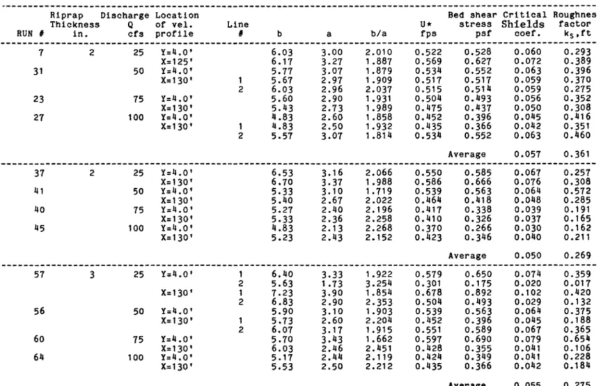
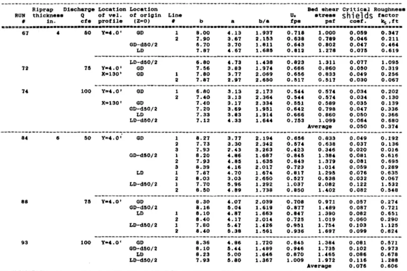
unit weight of water

The graphs of velocity distribution versus depth for incipient motion runs are presented in Appendix C {indicated by the run number). The calculated values of C and k are presented Tables 3.8 and 3.9. The values of C and k are obtained

CV S CV S

from the velocity profiles along the centerline of the flume {Y=4.0 ft) and across the middle section of the test reach {X=l25 ft for run No. 7 and X=130 ft for the rest of the runs). When the velocity profile lines were drawn through the data points adjacent to the riprap surface low values for C and k resulted. Examples are run _{CV S} No. 5 7 {Y =4.0 ft, line 112) and run No. 84 {Y =4.0 ft, line # 3) where C _CV

=

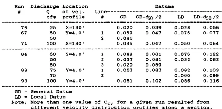
0.020.

To evaluate the effect of the bottom elevation on the logarithmic distribution of the velocity profile, a comparison was made between velocity profiles plotted using four different elevation datums. Two of these datums are the "general datum" {GO) and the "local datum" (LO) as defined in Chapter 2. The other two datums are selected to be a distanced /2 below the GO and LO (that is, GD - d /2 and LO -_{so 50} d 12). The velocity distribution for some selected runs (runs No. 67, 74, 76, 84, 88,

50

and 93) are plotted using these four datums. The graphs of velocity distributions for these runs are presented in Appendix C. As shown in these graphs, the data points adjacent to the riprap surface did not coincide with the velocity distribution line drawn through the remainder of the data points when the "local datum" was used. The effect of using these four different datums to evaluate the

bed Shields' coefficient C can be observed by referring to the values presented in

_CV

Table 3.10. These values indicate that the magnitudes of C are generally highest

_CV

when the LO - d

₅₀ /2

datum is used, and lowest when "general datum" is used. In the

next section, the values of C that are obtained using the "general datum" will be

_CV

-~~-~--~-~~~----~-~---~~--~~~---~----~---~~~--~~--~~-~~---·~--~-~--~--~---~-~--~-~----~-~--~---~~-Riprap Discharge Location Bed shear Critical Roughnes

Thickness Q of vel. Line U* stress Shields factor

RUN I in. cfs profile

'

b a b/a fps pst coef .. ks,ft

---~~~~---~---~-~-~-~---~~~~----~---~---~----~-~-~~-~---~---~---~~--~~~-~----~~~~--~·~ 1 2 25 Y::4.0' 6.03 3.00 2.010 0.522 0.528 0.060 0.293 X:125' 6. 11 3.21 1.887 0.569 0.627 0.012 0.389 31 50 Y::l4.o• 5.17 3.01 1.879 0.534 0.552 0.063 0.396 X=130' 1 5.67 2.97 1 .. 909 0.517 0.517 0.059 0.370 2 6 .. 03 2.96 2.037 0.515 0.514 0.059 0.275 23 75 Y:4.0' 5.60 2.90 1. 931 0.504 o.493 0.056 0.352 X=130' 5.43 2.13 1 .. 989 0.1475 0.437 0.050 0.308 27 100 Y:ll.O' 4.83 2.60 1.858 0.452 0.396 0.045 o.416 X=130' 1 11.83 2.50 1.932 0.435 0.366 0.042 0.351 2 5.57 3.01 1 .. 814 0.534 0.552 0 .. 063 o.46o Average 0.057 0.361 ---~~~---~--~---~-~-~~~--~~--~--~-~-~---~-~---~-~---~~-~--~~---~---~---~~-~---~---~-~---·-37 2 25 Y:4.o• 6 .. 53 3.16 2.066 0.550 0.585 0 .. 067 0.257 X:130' 6.70 3.31 1.988 0.586 0.666 0.076 0.308 41 50 Y:lf .O' 5.33 3.10 1. 719 0.539 0.563 0.064 0.572 X=130t 5.40 2.67 2.022 0.464 0.418 0.048 0.285 40 75 Y:4.0' 5.27 2.40 2.196 0.417 0.338 0.039 0.191 X=130' 5,.33 2.36 2.258 0.1110 0.326 0.037 0.165 45 100 Y=ll.o• 4.83 2.13 2.268 0.310 0.266 0.030 0.162 X=130' 5.23 2.'43 2.152 0.423 0.346 0.0110 0.211 Average 0.050 0.269 ---~~-~-~---~---~-~---~~---~----~---~-~~---~----~---~-~---~~---~---~---~-57 3 25 Y:4.0' 1 6.40 3.33 1 .. 922 0.579 0.650 0.074 0.359 2 5.63 1.73 3.254 0.301 0.175 0.020 0.011 X=130* 1 1.23 3.90 1 .854 0.678 0.892 0.102 0.1'20 2 6.83 2.90 2.353 0.504 0.493 0.029 0.132 56 50 Y:4.o• 5.90 3.10 1.903 0.539 0.563 0.064 0.375 X=130' 1 5.73 2.60 2.204 0.452 0.396 0.045 0.188 2 6.01 3.11 1.915 0.551 0.589 0.067 0.365 60 75 Y:4.0' 5.70 3.43 1.662 0.597 0.690 0.079 0.654 X=130' 6.03 2.46 2.451 o.428 0.355 0.041 0.106 614 100 Y=4.0' 5 .17 2.44 2 .119 0.424 0.349 0.041 0.228 X:130' 5.53 2.50 2 .. 212 0.435 0.366 o.M2 0 .. 184 Average 0.055 0 .. 275 --~---~~--~-~~~~--~~-~--~---~-~~----~---~~~-~----~~--~~~~--·~~----~~----~~~~--~----~-~~--~--~~--~-~--~---~-~

Table 3.8 Calculation of Bed Critical Shields

1

Coefficient Using Velocity Distribution

Equation for dso

=

1 in. Riprap.

N 0\

'

72 1' 84 6 88 93 2 7.90 6.70 'l.87 3.61 3.70 4.67 2.153 1.811 1.685 0.638 0.643 0.812 o.789 0.802 1.278 0.0'6 0.047 o.on 0.211 0.46' 0.619 75 100 50 75 100 Y•4.0' X•1301 GO-d50/2 LD LD-d50/2 GD GD 1 2 6,80 4.73 1.'38 7.56 3.83 1.97• 7.80 3.71 2.069 7.87 2.97 2.650 0.823 1.311 0.077 1.095 0.666 0.860 0.050 0.319 0.656 0.833 0.049 0.256 O.!U7 0.511 0.030 0.067 ---~---_{Y•4.0' GD 1 6.80 3.13 2.173 0.544 0.574 0.034 0.202} 2 7.40 3.13 2.364 o.su 0.514 0.034 0.130 X•130' GD 7.40 3.11 2.334 0.551 0.589 0.035 0.139 GD-d.50/2 7.20 3.69 1.951 0.642 0.798 0.047 0.336 LD 7.33 3.83 1.91' 0.666 0.860 0.050 0.366 LD-d50/2 ·z.12 4.33 1.64' 0.163 1.099 0.064 0.680 Average 0.050 0.374 Y•4 GD l 8.27 3.77 2.19• 0.656 0.833 0.049 0.192 2 7.73 3.30 2.342 0.$74 0.638 0 .03'1 0.136 3 7.93 2.43 3.263 0.423 0.346 0.020 0.016 GD-d50/2 1 8.20 4.86 1.687 0.845 1.384 0.081 0.616 2 7.93 4.85 1.635 0.8'3 1.379 0.081 0.695 3 8.39 4.16 2.011 0.723 1.014 0.059 0.289 LD 1 7.8'1 4.70 1.674 0.811 1.295 0.076 0.635 2 8.03 3.03 2.650 0.527 0.538 0.032 0.067 LD-d50/2 1 1.10 5.96 1.292 1.037 2.082 0.122 1.532 2 8.50 4.89 1.738 0.850 1.•02 0.082 0.548 -~---~---_{Y•4.0' GD 8.30 4.07 2.039 0.708 0.9'11 0.057 0.274} GD-d.50/2 8.16 5.04 1.619 0.877 1.'89 0.08'1 0.721 LD 1 8.10 4.87 1.663 0.847 1.390 0.082 0.651 2 8.40 4.17 2.014 0.725 1.019 0.060 0.290 LD-d50/2 1 7.80 5.47 1.426 0.951 1. 754 0.103 1.125 2 8.40 5.38 1.561 0.936 1.697 0.099 0.824 ~---~---_{Y•4.0' GD 8.36 4.86 1. '120 0.845 1.384 0.081 0.571} GD-d50/2 8.10 5.44 1.489 0.9'6 1.735 0.102 0.913 LD 8.23 5.00 1.646 0.870 1.465 0.086 0.678 LD-d50/2 1.93 6.80 1.367 1.009 1.972 0.116 1.288 Average 0.076 0.606 ---~---~---~--~---~--~---~---_GD

₌

_{General Datum} LD • Local Datum

Table

J.

9 Calculation of Bed Critical Shields' Coefficient Using Velocity Distribution Equation

for

d50

=

2

in. Riprap.

N '-I

28

Table 3 .10. Values of ~v for Some Selected Runs Calculated

Based on Four Different Datums

Run Discharge Location

# Q of vel. cfs profile Datums Line---# GD GD-~O I 2 LD LD-d50 I 2 ===========~===============================================··=======· 76 67 74 84 88 93 25 50 50 100 50 50 50 75 75 100 X=l30' Y=4.0' X=130' Y=4.0' Y=4.01 Y=4.0' GD

=

General Datum LD = Local Datum l 2 1 2 3 1 2 0.020 0.059 0.046 0.035 0.049 0.037 0.020 0.057 0.081 0.039 0.047 0.047 0.081 0.081 0.059 0.087 0.102 0.028 0.075 0.050 0.076 0.032 0.082 0.060 0.086 0.056 0.011 0.064 0.122 0.082 0.103 0.099 0.116

Note: More than one value of Ccv for a given run resulted from different velocity distribution profiles along a section.

3.4

Comparison

Of

The Values Of Critical Shields' Coefficients Calculated

By

The

Previous Three Methods

In Table 3.11 The calculated values of critical Shields' coefficient are presented

for comparison. The results show that values of bed critical Shields' coefficient

obtained using the Manning's friction factor (Ccn> have the lowest magnitudes and

those obtained by Prandtl-Von Karman equation (Cc) have generally (for

60%

of

the time) the highest magnitudes. However, some very low values of the Shields'

coefficient were obtained using the Prandtl-Von Karman equation.

The values of C that are presented in Table 3.11 were calculated based on the

CV

"general datum". As mentioned in the previous section, the values of C that were

CV

calculated based on the other three datums are higher than the ones obtained using

the "general datum" and, therefore, much higher than the values of C and C f.

_en

_c

Because of the wide range of values of Ccv (as shown in Tables 3.10 and 3.11), a

general conclusion cannot be made as if the values of Ccv represent the actual

values of bed critical Shields' coefficient or not. This raises the question of the

validity of the Prandtl-von Karman equation in predicting the shear stress on the

riprap surface, i:b, and, therefore, bed Shields' coefficient.

3. 5 Effect Of Flat Rocks

The l in. riprap contained about l 0 percent flat rocks. To determine the

influence of these flat rocks on the failure of the riprap, the flat rocks were

removed after the first series of tests and the tests were repeated.

No significant changes in critical Shields' coefficient were observed after

removal of flat rocks. The values of critical Shields' coefficient differ appreciably

only for a flow rate of 25 cfs (see Table 3.11 - runs No. 7 and 37). This difference is

probably due to the influence of the transition section of run No.

1

as mentioned

30

Table 3.11. Values of Critical Shields Coefficients Calculated by Different Methods Listed

Riprap Velocitydistrib

Run median Riprap Discharge Darcy Ccv

# size thicknes Q Overall Manning

Weisbach---in. in cfs

cc

ccn

ccf

@Y=4.0' @X=130 =================================================================~·===• 7 31 23 27 37 41 40 45 1 1 2 2 25 50 "i 5 100 100 25 50 75 100 0.044 0.051 0.046 0.053 0.056 0.046 0.047 0.059 0.041 0.045 0.040 0.045 0.053 0.041 0.041 0.051 0.043 0.048 0.042 0.048 0.054 0.043 0.043 0.054 0.060 0.063 0.056 0.045 0.067 0.064 0.039 0.030 0.072 0.059 0.050 0.042 0.063 0.076 0.048 0.037 0.040

---

_{57 1 3 25 0.066 0.063 0.064 0.074 0 .102} 25 0.020 0.033 56 50 0.057 0.052 0.054 0.064 0.045 50 0.067 60 75 0.067 0.060 0.063 0.079 0.041 64 100 0.067 0.058 0.062 0.041 0.042

---·---

_{67 2 4 50 0.055 0.049 0.052 0.059} 50 0.046 72 75 0.049 0.041 0.045 0.050 75 74 100 0.058 0.047 0.053 0.034 84 2 6 50 0.067 0.059 0.063 0.049 50 0.037 50 0.020 88 75 0.068 0.058 0.064 0.057 93 100 0.074 0.061 0.068 0.081

Note: More than one value of Ccv for a given run resulted from different velocity distribution profiles along a section.

0.049 0.030 0.035

}.6

~

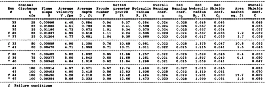
ffect Of The Riprap Thickness On Critical Shields' Coefficient(C c)

The failure criterion for riprap was the exposure of the filter blanket after a

run. For a given discharge, the run at which the flume slope was one increment

lower than the failure run was regarded as the incipient failure run from which the

critical Shields' coefficient was calculated. Based on the above definition of the

incipient failure run, it was expected that the riprap with greater thickness would

have higher values of critical Shields' coefficient. This is because the Shields'

coefficient is used to define a point that is the result of a significant amount of

motion of the riprap even prior to what is defined as a failure.

The values of critical Shields'

coHffidtmt,

C , are presented in Table 3.l

_c

l.

These values show that, on the average, the critical Shields' coefficient increased 22

percent for l in. rocks and 30 percent for 2 in. rocks when rock thickness increased

from 2d

₅₀

to 3d . The values of overall critical Shields' coefficient calculated

₅₀

from equation (3.7) (Cc) are plotted in Figure 3.l. The increase in the critical

Shields' coefficient as shown in Figure 3.1 was relatively small when the rock size

increased from 1 in. to 2 in. (4 percent on the average) and the thickness remained

at 2d . However, the critical Shields' coefficient increased about 30 percent when

50

d

₅₀

in.

Thickness in.

0

I

2

•

I

3

0

_...

0.07

l:l.

2

4

6

t-

...

₂

·----·

z

•

L&J

•,

/

-0

/

-...

'

/

...

L&J

'

/

0

'

0

/

0.06

'

/

0

I

w N Cf) Q

'-/

_.

LtJ

o,

-:c

(/)

"

_.

'

<(

'

0

_0.05

-'

t-

_-/

-a:

"

--- .---0

0

o----50

0.040

DISCHARGE,

cfs

75

100

3.7 Effect of Riprap Gradation on Critical Shields' Coefficient (C )

_c

To examine the effect of gradation, values of overall critical Shields'

coefficients are plotted in Figure 3.2 for the riprap materials presented in Table

3.12. The values of d /d are used as the parameters to represent the gradation

_{as 1s}

of riprap material. The values of d /d in Table 3.12 indicates that the riprap

_{85 15}

material of this 1985 Study and the 2 in. riprap of the 1982 Report had a more

uniform gradation than the 1 in. riprap of the 1983 Report.

As shown in Figure 3.2, the range of values of the critical Shields' coefficients for l

in. riprap of the 1983 Report was lower than the rest of data points. These results

show that a riprap with more uniform gradation is more stable. Additional data are

required

to

generalize the effect of gradation on riprap stability.

TABLE 3.12 Gradation of the Riprap Material

d in

_so

Riprap Thickness

d /d

_K-.

₁₅

Y car of Study

l

2

2.0

1985

1

2

4.4

198}

2

4

2.4

1985

0

u

I-z

IJJ

u

lJ... lJ... IJJ 0

u

-

CJ) 0 _J IJJ

-:c

CJ) _J <(

u

i=

-a:::

0

O.OGO.---,---r~---,..---0.055

0.050

0.045

0.040

0.035

4/+

"~·

_~0.0

"~

'\:? ••

••

·.

_·.

..

_·

_.

_..

··.

"'

·~Jl

,.,.'l:> ••

,.,,

_.·

.

~e;q_:·/

.·. /

A_,q ••

..

~

.·

"'···

/

~·· •

··.'\]'···/

n---_d

0

II _... ...

~~

!£~£.! .!..9!~..o--

.. ./

,.,,0

,..,,,,,,.,,,,,,.

0.03u---'---.L.---L---1---'

₀

₂₅

₅₀

₇₅

₁₀₀

DISCHARGE,

cfs

Figure 3.2 Variation of overall critical Shields' coefficient with riprap qradation.

w

3.8

Comparison With Shields' Diagram

Shields' diamgram is an experimental relationship between the values Shields'

coefficient for incipient motion runs (C .

_Cl

=

i: /( y _{C W}

(s-1 )d)) and grain Reynolds

number CR* = U*d/\>) where U* is shear velocity in fps, dis particle size in ft, and

\) is kinematic viscosity in ft

2

_{/sec. Shields assumed that for a flat bed of uniform}

particle size, C ci is only a function of R* (Rouse,

1950).

Shields' diagram is shown

in Figure 3.J. Shields determined this relationship by measuring the washed out

mterial (bed load) at various values of

i:/(y _w

(s· l) d) at least twice as large as the

critical value (C . ) and then extrapolating

to

the point of zero washed out material

Cl

(Gessler,

1971 ).

Gessler (

1971)

argued that some of Shields bed load measurements

were under conditions where ripples and small duens prevailed, and therefore the

shear stress on bed was resisted by both bed deformation and grain roughness.

Gessler concluded that values of C ci determined by Shields were up to 10 percent

too high. Gessler modified the Shields' diagram as shown in Figure

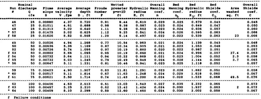
J. }.

To compare the results of this riprap stability study with Shields' diagram, the

values of overall critical Shields' coefficient (Cc) versus boundary Reynolds' number

(Rx

=

u.

d

I

u} are presented in Table

3.13

and plotted in Figure J.J. In this

50

figure, the values of C from the 1982 and

_c

1983

Reports are also plotted. Note that

the original Shields' diagram was constructed using the values of Shields' coefficient

for incipient motion runs but values of C are for the incipient failure runs. the

_c

scatter of data points in Figure

3.3

are most probably due to two reasons: l) In

incipient failure runs some of the riprap material may move without exposing the

underlying filter blanket. this is more pronounced in rirpraps with grHater

thicknesses. As shown in Figure

3 .. 3,

the values of C for Jd thickness riprap are

_c

'50

greater than the Shields' coefficient of

0.06.

2) The riprap materials were not

36

The data points in Figure 3. 3 indicate that the values C obtained from the

_c

recent study are generally higher than those of the previous reports. There is some

overlap between the C values of the 2 in. riprap of 1982 Report and the recent

_c

data. Agreement does not exist for l in. rocks of the 1983 Report and the present

study. There is a pronounced difference between the critical Shields' coefficient,

C ,

_c

based upon the riprap thickness of 2d and 3d . The variations in

_{so so} Cc

among

various ripraps can

be

attributed to the differences in thicknesses and gradations of

the riprap material. As discussed in section 3.6, it is expected that a riprap with

greater thickness requires greater bed shear stress (or Shields' coefficient)

to

begin

to fail. the influence of gradation was discussed in section 3. 7. The difference in

C values for 1 in. riprap (2d thick) of the 1983 Report and the present study may

_c

_so

be because of the differences in gradations of the ripraps. Some of these

discrepancies are also because of the procedure to change the flume slope to reach

the incipient failure run. The actual point of incipient failure could occur at a µoint

where the slope was between that slope called failure and that slope

SHI.

one

increment lower than failure.

3. 9

Ma~imum

Stable Slopes At The Incipient Failure Runs

The slopes of the incipient failure runs versus flow rate are plotted in

Figure 3.4. This figure also contains the information from the previous report. No

general conclusion can be drawn from this plot.

Table 3.13. Values of

cc

and R*

~-~--~---~---~~---~---~~--~---~-~~---~-~~----Riprap

median Riprap

Discharge

size thickness

Q

in.

in.

cfs

1 l 1 l 2 2 2 2 25 50 75 100

Run

# 7 31 23 27

Overall

Shields

coef.

Cc 0.044 0.051 0.046 0.053

Boundary

Reynolds

number

R-k 3725 3979 3802 4077

---

_l l 1 1 1 l l l 2 2 2 2 2 2 2 2 2 2 3 3 3 3 4 4 4 6 6 6 25 50 75 100 25 50 75 100 50 75 100 50 75 100 37 41 40 45 57 56 60 64 67 72 74 84 88 93 0.056 0.046 0.047 0.059 0.066 0.057 0.067 0.067 0.055 0.049 0.058 0.067 0.068 0.074 4186 3791 3847 4296 4540 4220 4579 4584 11580 10921 11920 12768 12914 13438

E <,_l (.) ... z w 0 LL u... w 0 (.) (I') 0 ...J w :z: (f) ...J <t (.) ... a:: (.) 1.0

t

_2d50 0 0 A \I 0.1~ 3dso

•

25 cfs

•

50 cfs

•

75 cfs

•

I 00 cfs Original Shields' Curve + + 1985 Doto ,,' ,,""

~

o o Ranoe of

_

_

_ci::!!!:!..60:::::...

.b"' ~b.,

1985 Doto

---.

~---_s.:Q:..O~~

_{Gess\er's Modificotion} A _{o ---,---}~

----

0 <# - -_-+A

v::---

---NO M o aon t' _" '\.v

~-

~

.b. .v ,, hJ ₀ ~ .~ b4' Motion ~ b~ t I t I I t I I I I I I I I I I I I I I I !

fJ

0.01

i

I I I I I I . ~o·

.

I I • I I I '102 I I I I '10s 104 105 CD BOUNDARY REYNOLOS1 NUMBER

R.

=

v.d 50 1'

Figure 3.3 The Shields' DiaQram

=

/gDS dso _v

w

0.020---..,---IJJ a. 0.018

o.o

16

o.o

14

9 o.o

12 (/) IJJ _..J m <t

_....

(/)

o.o

10 2 ::::> 2

_x

_0.008 <t 2 0.006 0.004 0.002 25 50 75 100 DISCHARGE, c.fs

40

CHAPTER4

SUMMARY, CONCLUSIONS AND RECOMMENDATIONS

A total of 94 tests were conducted on riprap with d =l in. and d =2 in. and

_{so so}

with thickness layers of 2d and Jd • The flow rates tested were 25, 50, 75, and

_{so so}

100 cfs. The tests were conducted in the 8 ft tilting flume of the Hydraulics

Laboratory, Engineering Research Center of Colorado State University. For each

riprap and each flow rate the flume slope was increased by small

incremen~.s

until

the failure of the rip rap occurred. The exposure of the filter blanket underneath the

riprap was the failure criterion. The run with the flume slope reduced one

increment lower than the slope at failure was considered to be the incipient failure

run. Velocity data were collected either by ott meter or pitot tube. The data are

presented in the Appendices.

The following conclusions are made in this study.

1.

The average values calculated for bed Manning's roughness, nb, agree with

the ones calculated by Anderson et al. equation. Strickler equation

underestimates the bed Manning's roughness factor.

2.

The values of bed Shields' coefficient at the incipient failure conditions

range from 0.041

to

0.054 for riprap placed 2d thick and range from

_so

0.052 to 0.068 for riprap placed Jd

_so

thick. The above valutts are

Shields' coefficients calculated using velocity distribution equations,

range from 0.020 to 0.102. These differences result from local flow

patterns and velocity distributions.

3.

No general relationship exists between maximum stable slope and rock

size for a given flow rate. There is a trend of the maximum slope

increasing with riprap size as shown in Figure 3.4.

4.

Generally, The wide range of the results is most likely due to the wide

variation in gradations and thicknesses of ripraps.

The recommendations are generally similar to the ones presented in the 1982

and 1983 Reports. It is suggested that a small portion of the riprap be painted and

placed in a grid on the surf ace of the rip rap. Displacement of a percentage of

painted rocks, then can be used to define the incipient motion or incipient failure

runs. Some means should be designed to observe the behavior of the painted rock

during a test, for example, using a video camera and recorder.

42

Rt.I- ERENCES

1. Anderson, A.G., A. S. Paintal, and J. T. Davenport, 1970. Tentative Design

Procedure for Riprap-Lined Channels: National Cooperative Highway

Research Program Report 108, Highway Research Board, National

Research Council, National Academy of Science, 75 p.

2. Chow, V. T., 1959. Open Channel Hydraulics. McGraw-Hill Book Company, Inc.

New York, New York.

3. Department of Army - Corps of Engineers. Hydraulic Design of Flood Control

Channels. Manual EMl 110-2-1601, July, 1970.

4. Fiuzat, A. A., Y. H. Chen, and D. B. Simons, 1982. Stability Tests of Riprap in

Flood Control Channels. Report No. CER81-B2AAF -YCH-DBS56, Dept.

of Civil Engineering, Colorado State University, Fort Collins, Colorado,

October.

5. Fiuzat, A.A. and E. V. Richardson, 1983. Supplemental Stability Tests of Riprap

in Flood Control Channels. Draft Report CER83-84AAF -EVRlB, Civil

EnglnHHring Department, Colorado State University, Fort Collins,

Colorado, December.

6. Gessler, J ., 1971. Beginning and Ceasing of Sediment Motion, River Mechanics

edited by H. W. Shen, Chapter 7, Fort Collins, Colorado.

7. Rouse, H. {1950), Ed., Engineering Hydraulics, John Wiley

&

Sons, New York,

p.

790.

8. Shields, A., 1936. "Anwendung der Aehnlichkeitsmechanik und Turbulenz

F orschung auf die Geschiebebewegung," Mitteilung Preussiche

Versuchanstalt Wasser, Erd, Schiffbau, Berlin, No. 26 (in German), cited in

D. B. Simons and F. SHnturk, 1977. Sediment Transport Technology,

Water Resources Publications, Fort Collins, Colorado.

9. Simons, D. B. and F. Senturk, 1977. Sediment Transport Technology. Water

Resources Publications, Fort Collins, Colorado.

10. Vanoni, V. A., ed. 1975. Sedimentation Engineering, ASCE, 345 East 47th St.

New York, New York.