Temporal partitioning of a chlorinated solvent release between transmissive and low permeability zones

Temporal Partitioning of a Chlorinated Solvent Release Between

Transmissive and Low Permeability Zones

A. Bolhari and T. Sale

Department of Civil and Environmental Engineering, Colorado State University

Abstract. This paper explores the hypothesis that chlorinated solvent releases evolve temporally

and spatially. A two-layer system is considered involving a transmissive layer (e.g. sand) situated above a low permeability layer (e.g. silt). A DNAPL like source is present in the transmissive layer at the upgradient edge of the model domain at the contact between the two layers. A constant source is active for 1000 days. Subsequently the source is shut off and the problem is studied for an additional 2000 days. Total contaminant mass in transmissive and low permeability layer along with total mass in selected profiles of the soil are evaluated. Calculations also take into account the effect of retardation. At 1000 days, with no retardation in the low permeability zone, 32% of the released contaminant mass is present in the low permeability layer. Given the same conditions and retardation factor of 10 in the low permeability zone, 58% of the released

contaminant is present in the low permeability layer after1000 days. Overall, the results illustrate that the nature of the problem evolves from one of dense non-aqueous phase liquids (DNAPLs) in the transmissive layer at early time to one of aqueous and sorbed phases in the low permeability layer at late time. Understanding the evolutionary status of a release can be a key factor in selecting remedies. Furthermore, results indicate that the distribution of contaminants in the low permeability zone evolves with time. This supports the observation that the domain in which significant contaminant mass is present in low permeability zone can be a subset of the overall plume. Critically, this observation suggests that treatment of contaminants in low permeability zones can be limited to a subset of the overall plume domain.

1. Introduction

At many sites, chlorinated solvents were historically released into subsurface setting in the form of dense non-aqueous phase liquids (DNAPLs). With time, DNAPL constituents partition into water, sorb to solids, and partition into soil gas. Following Feenstra et al. (1996) and Kueper and McWhorter (1991), DNAPLs preferentially move through the most transmissive portions of subsurface media and frequently come to rest above low permeability zones. Entry of DNAPL into low permeability zones is often precluded by insufficient capillary pressures (pool height) to displace the water from the pore spaces in low permeability zones. As such, DNAPL is most often found in the transmissive portions of source zones. An important exception can be secondary

permeability features in low permeability zones (e.g. root cast and slickenslides) that have large opening and relatively lower entry pressures.

With time, DNAPL constituents partition into the aqueous phase and advection carries the dissolved phase downgradient through transmissive intervals creating dissolved phase plumes. Herein, transmissive zones are conceptually defined as intervals in which advection is a primary transport process (seepage velocities > 1 m/year). In evaluating 88 sites, Newell et al., (1990) reports a median plume length of 1,000 ft for chlorinated

ethenes. Concurrently, vapor phase plumes can form in unsaturated zones via direct evaporation of DNAPL in unsaturated zones or partitioning from aqueous phases.

A potential consequence of DNAPL dissolution and constituent advection is the formation of large concentration gradients at the contacts between transmissive and low permeability zones (Sudicky et al. 1986, Chapman and Parker 2005, Parker et al. 2008, and Sale et al. 2008). Herein, low permeability zones are conceptually defined as intervals in which advection is a weak process (seepage velocities <1m/yr). With time large

contaminant concentration gradients at contacts between transmissive and low permeability zones drive dissolve phase constituents into low permeability zones via diffusion. Processes that can enhance diffusive transport into low permeability zones (by increasing concentration gradients) include sorption (Parker et al., 1994) and degradation (Sale et al., 2008). Assuming insignificant advective transport, dissolved phase

constituents will continue to move across contacts from transmissive to low permeability zones as long as the dissolved phase constituent concentrations are greater in the

transmissive zone. Conversely, given concentrations in transmissive zones, at contacts, that are less than concentrations in low permeability zones, diffusion can drive release of constituent from low permeability zones.

A number of researchers have recognized that contaminant stored in low

permeability zones can sustain plumes with adverse contaminant concentrations long after mass flux from the original DNAPL source is depleted. Liu and Ball (2002) observed a slow release of chlorinated solvents from an aquitards after a source removal from an overlying sand unit. Chapman and Parker (2005) illustrated sustained releases from a low permeability unit to an overlying transmissive sand 6 years after the original DNAPL source zone was isolated from the plume using a physical barrier. Furthermore, Chapman and Parker (2005) employed high resolution numerical modeling methods to demonstrate that releases from low permeability zones can sustain adverse concentration in a

transmissive zone for 100 years after source isolation. Sale et al. (2008) advanced an analytical solution for a two layer system consisting of a semi-infinite transmissive zone overlying a semi-infinite low permeability layer with a constant DNAPL like source in the transmissive zone. Figure 1 presents the conceptual frame work of the two layer model. Results presented in Sale et al. (2008) show that releases from low permeability zones is a function of position downgradient of the original source, retardation in the low

permeability zone, and rates of degradation in the low permeability zone.

Analytical solutions of advective-dispersive equation have been widely applied to describe solute transport in porous media. Early studies such as Skopp and Warrick (1974) and Al-Niami and Rushton (1979) neglected the effect of retardation. Tang et al. (1981) studies single thin fracture whereas Sudicky and Frind (1982) considered system of parallel thin fractures. Others focused on transient one-dimensional (Cameron and Klute, 1977) or steady three-dimensional transport (Sale and McWhorter, 2001). All these studies considered relatively narrow aspects of a much larger problem.

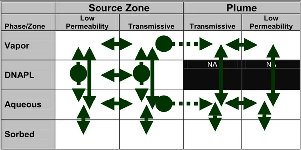
Building on all of the above noted concepts, Sale and Newell (2011) developed the 14 Compartment Model (Figure 2) as a tool for identifying all of the potential

combinations of contaminant phases in transmissive and low permeability zones, in source zones and plumes. Furthermore, the 14 Compartment model can be used to map

contaminant fluxes between the compartments and anticipate the benefits of remedial measures.

Figure 1. The two-layer scenario conceptual model: A) Active source, B) Depleted source (after Sale et al., 2008).

Figure 2. Contaminant phases in transmissive and low permeability zones. Arrows: potential mass transfer between compartments. Dashed arrows: irreversible fluxes (after Sale and Newell, 2011).

The 14 Compartment model uses the NRC (2005) definition of a source zone - a zone in which a DNAPL was released that can include contaminants stored about the original DNAPL release. Conversely, by exclusion, the 14 Compartment Model definition of a plume is contaminated zones in which DNAPL was never present.

The objective of this paper is to illustrate the evolution of a chlorinated solvent release through time per the concepts advanced in the 14 Compartment Model. More specifically, the objective is to resolve the distribution of contaminant mass in critical compartments as a function of time and position. Following Sale and Newell (2011), the distribution of contaminant mass in compartments is seen as a potentially critical aspect of selecting remedies and anticipating associated benefits. Furthermore, the distribution of contaminant mass in compartments is seen as a problem that varies in both time and space. As such, the position in the body of a chlorinated solvent release and the age of the release can play an important role in selecting appropriate remedies.

Source Zone Plume

Phase/Zone Permeability Low Transmissive Transmissive Permeability Low

Vapor DNAPL

NA NA

Aqueous Sorbed

Semi-infinite low permeability zone (e.g. silt)

Groundwater flow B ) y x

Plume of aqueous-sorbed contaminants

Semi-infinite transmissive zone (e.g. sand) A

This paper employs the two-layer scenario and analytical solutions developed in Sale et al. (2008) to estimate contaminant mass present in selected compartments as a function of time, position, and retardation in the low permeability zones. Given the fact that the Sale et al. (2008) analytical model only addresses saturated media, vapor phase compartments are excluded from the analysis. An important constraint to using the Sale et al. (2008) Mathcad worksheet is that it only works for domains less than 100 m in transmissive zone. Beyond 100m the Sale et al. (2008) Mathcad worksheet runs into computational problems. A partial solution is found to this problem wherein a series approximation is used for those portions of the domain where the Sale et al. (2008) Mathcad worksheet fails. The

combined series - Sale et al. (2008) Mathcad worksheet approach is referred to as the hybrid solution. Unfortunately, the hybrid approach also has a limited domain of

application. In the end, the manuscript relies solely on the low permeability layer solution from Sale et al. (2008) which can be applied to large domains. Contaminant mass in transmissive zones is estimated as the difference between the mass released from the source and the mass in the low permeability zone. Currently, further study is ongoing at Colorado State University to find practical computational approaches for the Sale et al. (2008) transmissive zone solution.

2. Modeling

Analytical solutions described in Sale et al. (2008) were used to estimate the distribution of DNAPL, aqueous and sorbed phase in transmissive and low permeability zones as a function of time. These solutions were employed to address two main questions or concerns: 1) temporal partitioning of the contaminant between transmissive and low permeability zones and 2) spatial variation in mass in low permeability zones. These questions are explored in two scenarios. The first scenario assumes no retardation in either layer. The second scenario includes a retardation factor of 10 for the low permeability zone. All calculations were carried out using MathcadTM 14. The following describes modeling assumptions, computational approach, and model limitations.

2.2 Assumptions

The physical setting of the two-dimensional (2-D) two-layer system considered in this modeling effort was previously introduced in Figure 1. The transmissive layer is situated above the low permeability layer. A DNAPL like source exists at the contact of the two layers. Primary assumptions are as follows:

1) A one-dimensional (1-D) advective flow parallel to the boundary of the layers accompanied by transverse diffusion/dispersive flow in transmissive layer,

2) A 1-D transverse diffusion in low permeability layer (no advection- the hydraulic conductivity of the transmissive layer is rather small resulting in molecular diffusion as the solute transport mechanism),

3) Transmissive and low permeability layers are uniform, homogeneous and isotropic,

4) No degradation is considered in either layer,

5) Transmissive and low permeability layers are semi-infinite,

In more detail, initial and boundary conditions include: ( , ,0) 0 c x y = (1a) '( , ,0) 0 c x y = (1b) ( , , ) 0 c x y→ ∞ = (2a) t '( , , ) 0 c x y→ ∞ = (2b) t ( ,0, ) '( ,0, ) c x t =c x t (3a) * ' ( ,0, ) ' ( ,0, ) t c c nD x t n D x t y y ∂ ₌ ∂ ∂ ∂ (3b) where, c(x,y,t), n and Dt are solute concentration, porosity and effective transverse

diffusion coefficient of the transmissive layer and c`(x,y,t), n` and D* are solute concentration, porosity and effective transverse diffusion coefficient of the low permeability layer, respectively.

The source term which is only present at the inlet (x=0) is modeled as: 0

(0, , ) by[1 ( `)] ( 0)

c y t ₌c e− ₋H t t₋ y_{≥ (4)} where b is the source distribution constant chosen in Sale et al. (2008) such that the model solute loading matches the solute loading in their experiments. In Equation (4), t` is the persistence time of the solute source and H is the Heaviside step function, such that:

0 ` 1 ` ( `)

{

if t t if t t H t t ≤ > − = . (5)

All input values of the model are presented in Table 1 and are based on common conditions found in alluvial setting.

Table 1. Input parameters of the model

Parameter Values Units

Average linear groundwater velocity, v 0.27 m/day

Porosity of the transmissive layer, n 0.25 dimensionless

Porosity of the low permeability layer, n` 0.4 dimensionless

Hydraulic conductivity of the transmissive layer, k 1.4×10-4 _m/s

Hydraulic conductivity of the low permeability layer, k` 1.7×10-6 _m/s

Aqueous solubility of PCE, c0 240 mg/L

Retardation factor of the transmissive layer, R 1 dimensionless

1_{Retardation factor of the low permeability layer, R` 1 and 10 dimensionless}

Effective transverse diffusion coefficient of the transmissive layer, Dt 4.5×10-9 m2/s

Effective transverse diffusion coefficient of the low permeability layer, D* _5.5×₁₀-10 _m2_/s

1_{Retardation factor of the low permeability layer is 1 for scenario 1 and 10 for scenario 2.}

In this study the source is on for 1000 days (t`) and then shut completely off

allowing clean water to flush through the media for an additional period of 2000 days. The source has a concentration of c0=240 mg/L at the interface of two layers at x=0. The

aqueous concentration associated with the source decays exponentially with increasing distance above the interface of two layers in the transmissive layer (see Figure 1). The

source term b and c values used in this study are based on 1m thin pool of _o perchloroethene (PCE) located upgradient of the point x=0 and y=0.

In Table 1 the effective transverse diffusion coefficients of PCE in transmissive and low permeability layers (D and_{t D}*_{) are respectively defined as:}

t t e D =vα + (6a) D 1 * _'3 aq D =n D (6b) where, D , the effective molecular diffusion coefficient of PCE in transmissive layer is _e calculated from:

1 3

e aq

D =n D (6c) In the above equations, α_t =0.0013m is the coefficient of transverse hydrodynamic dispersion and _{7.5 10}10 2

aq m

D _{= ×} − _{s is the aqueous diffusion coefficient of PCE.} 2.3 Computational Approach

Contaminant concentrations in the transmissive and low permeability layer at a desired location and time are calculated from Equations (7)-(10), per Sale et al. (2008):

2 2 2 2 . 0 0 _{2 2} 1 ( , , ) ( [ ( ) ( )] 2 2 2 2 ) ( ) ( )) b x by by by trans b x by c c b y b y c x y t c e e erfc x e e erf x x x b y erfc x e e t x v x _{x t} v φ ξ φ φ φ φ φ φ ξ φ ξ φγ π _{ξ γ ξ φ} − − − = + + + + ⎛ ⎛ ⎞ ⎞ + ⎜ ⎜_⎜ ⎟_⎟ ⎟ − ⎜ ⎝ ⎠ ⎟ + − _{⎜ ⎟} − _{⎜ − + − ⎟} ⎜ ⎟ ⎝ ⎠

∫

(7)

where, φ, γ and vc are defined as:

t v D φ= (8a) * ' ' t n R D n D γ = (8b) c v v R = (8c) and R and R` are retardation factors of the transmissive and low permeability layer, respectively. 2 2 1 0 ₀ ( , , , ) 1 1 ( , , ) ( [ ( )] ) b x low k I x y t b b c x y t c e erfc d x ξ φ ξ _{ξ ξ} φ φ π ξ πξ = − −

∫

(9) where,

* 2 2 * 1 2 2 * 2 2 2 2 ` ( ) 2( ) ` ( , , , ) ( ) 2 ( ) ` exp[ ] 4( ( ) ( )) c c c c c c y D R erfc y x t x v x D _t v R I x y t erfc y x t D v x _R t x x v _t x _{x t} v v γ γ φ ξ ξ γ φ γ φ ξ _{γ ξ φ} − + − − = − − − + − − − + − (10)

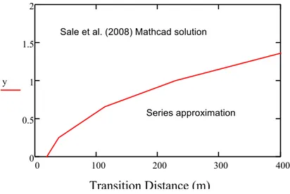
Concentration contours generated using a Sale et al. (2008) Mathcad worksheet is presented in Figure 3. Also shown in Figure 3 are concentration contours generated using a Hybrid method that is described in the following text. Concentrations in Figure 3 are presented in mass of PCE per volume of water. Unfortunately, Sale et al. (2008) Mathcad worksheet for transmissive layer does not result in accurate values for larger plume lengths (greater than 100m). Consequently, the Sale et al. (2008) Mathcad worksheet for Equation (7) has a finite domain of application. The distance at which the Sale et al. (2008)

Mathcad worksheet approach fails is referred to as the transition distance.

Nx=200 Ny=50 Δx=2 Δy=0.04 Nx=200 Ny=50 Δx=0.5 Δy=0.01 Grid size Hybrid method

Sale et al. (2008) Mathcad solution

0 50 m 100 m 0.5 0 -0.5 m mg/L sand low k transmissive 0.5 0 -0.5 m 0 50 m 100 m mg/L transmissive low k low k 0 200 400 m 2 0 -2 m transmissive mg/L 0 200 400 m low k transmissive mg/L 2 0 -2 m

Figure 3. Predicted concentration contours in 1000 days from Sale et al. (2008): panels A and B, and hybrid method: panels C and D.

C A

For larger distances an alternative computational strategy is required. For this research, a series expansion was used to approximate

2 2 2 b x b y e erfc x x φ φ φ ⎛ ₊ ⎞ ⎜ ⎟ ⎝ ⎠ and 2 2 1 2 b x b y e erf x x φ φ φ ⎛ ₊ ⎛− ₊ ⎞⎞ ⎜ ⎜ ⎟⎟ ⎝ ⎠

⎝ ⎠ in Equation (7). These series are summarized in Appendix 1

and Appendix 2. Unfortunately, series are incorrect at small distances. Realization of the limitation of both the Sale et al. (2008) Mathcad solution and the series approximation lead to a strategy of using each of the approaches in the domain where they are accurate. This approach is referred to as the hybrid method. In this method, the Sale et al. (2008) Mathcad worksheet solution is used for distances less than the transition distance and series approximation is used for distances greater than the transition distance. Using the hybrid approach, concentrations are evaluated over the domain of interest at Nx points in

the x direction and Ny points in the y direction. The distances between the points are Δx

and Δy. The distance y increases upward in the transmissive layer and downward in the low permeability layer. The Transition Distance can be solved for numerically by

employing Mathcad’s programming loop for a desired Δx and y (vertical distance from the interface of two layers in the transmissive layer). The loop reports the transition distance when the results from Equation (7) and its equivalent series approximation differ less than 0.2%. The red line in Figure 4 shows the Transition Distance for a desired y in the

transmissive layer when Δx=0.1 m and Nx= 200. The area above and below the red line,

respectively indicates the domain where Sale et al. (2008) Mathcad worksheet solution and the series are applied.

Therefore, c_{low k}( , , )x y t and the modified c_trans.( , , )x y t can be employed to calculate contaminant concentrations in transmissive and low permeability layers in larger desired location and time by departing from Sale et al. (2008) solution to the series expansion. For instance, Figure 3 (panel B) reflects concentration contours generated from Sale et al.

0 100 200 300 400 0 0.5 1 1.5 2 y Transitionalx 0.1 y( , )

Figure 4. Transition distance calculated for Δx=0.1 m and Nx=200.

Transition Distance (m)

y (m

)

Sale et al. (2008) Mathcad solution

(2008) versus the hybrid method (panel D) in 1000 days and the domain size of Lx= 400 m

and Ly= 4m. Panel C also illustrates the same scenario as panel A, but through hybrid

method.

One of the applications of the model is to predict total contaminant mass in transmissive and low permeability layers. Mathcad’s numerical integral scheme was employed to calculate the total mass in the transmissive and low permeability layers as follows in Equation (11a-b).

.( , , ) _{0 0} 0 .( , , ) y x N y N x trans trans M Δ Δx y t =

∫ ∫

Δ Δ nRc c x y t dxdy (11a) 0 0 0 ( , , ) N yy N xx ' ' ( , , ) low k low k M Δ Δx y t =

∫ ∫

Δ Δ n R c c x y t dxdy (11b) Unfortunately, hardware and/or software limitations resulted in floating point error and cease of operations in the transmissive layer solution due to insufficient computer memory for distances larger than 689 m. This resulted in calculation failure following a prolonged attempt to run calculations (over 24 hours). Therefore, total PCE concentration in the low permeability layer at a desired time of t and a grid spacing of ∆x and ∆y is evaluated during the loading (Equation 11c) and back diffusion (Equation 11d) as follows:

0 0 0 ( , , ) ' ( ' ( , , )) y x N N low k low k j i M x y t x y n R c c i x j y t = = Δ Δ = Δ Δ

∑ ∑

Δ Δ (11c) _ 0 0 0 ( , , ', ) ' ( ' ( , , ', )) y x N N

low k back diffusion low k

j i

M x y t t x y n R c c i x j y t t

= =

Δ Δ = Δ Δ

∑ ∑

Δ Δ (11d)

where, t` is the source persistence time, i and j are integer counter variables and

( , , )

low k

c i x j y tΔ Δ is calculated from Equation (9). To minimize errors associated with spatial discretization of the domain, fine discretization (Nx and Ny of up to 11000 and

5000, respectively) and a grid spacing as tight as ∆x=0.1 m and ∆y=0.001 m were used. These values were chosen iteratively with the goal of a mass balance error of less than 0.1% (see Appendix 3).

The total contaminant mass in the system as a function of time is defined by integrating the influent flux of contaminants at x=0 over y and over time.

0 0 0 ( ) t by source M t ₌ ∞vnc e dydt−

∫ ∫

(12) The contaminant mass in the transmissive layer is determined as the difference between total mass that entered the system at x=0 (Equation 12) and the total contaminant mass in the low permeability layer (Equations 11c and 11d).

( , , ) ( ) ( , , )

transmissive source low k

M Δ Δx y t =M t −M Δ Δx y t (13) Another application of the model is to predict aqueous and sorbed mass through select vertical columns (transects) in the low permeability layer at select times. Mass in transects during the loading and back diffusion are calculated, respectively, as:

sec 0 0 ( , , ) ' ( ' ( , , ) y N tran t low k j M x y t x y n R c c x j y t = Δ Δ = Δ Δ

∑

Δ (14) sec _ 0 0 ( , , ', ) ' ( ' ( , , ', ) y N

tran t back diffusion low k

j

M x y t t x y n R c c x j y t t

=

Δ Δ = Δ Δ

∑

Δ (15)

where, M_{transec _t back diffusion}( ,Δ Δx y t t, ', ) is the total mass and c_{low k}( ,x j y t tΔ , ', ) is the PCE aqueous concentration in the low permeability from back diffusion (after source is shut down).

One of the limitations of this method is that contaminant mass in the transmissive layer is determined indirectly through subtraction of the contaminant mass in the low permeability layer from the total contaminant mass introduced to the system. Another limitation is that degradation of contaminants is not addressed in either transmissive or low permeability layers. Lastly, the analytical model only addresses saturated media excluding vapor phase compartments from the analysis.

3. Results

3.1 Temporal partitioning between transmissive and low permeability zones 3.1.1 Scenario 1: without adsorption

Figure 5 and Figure 6 illustrate the case where no adsorption occurs in the

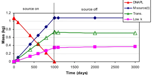
transmissive and low permeability layers (retardation coefficients of 1). The PCE DNAPL source is on for 1000 days and completely off for 2000 days. Contaminant mass is

reported in kilograms per 1 meter width of the porous media over the entire domain impacted by the source. In Figure 5 accumulated PCE mass in the system, Msource(t),

increases with time following Equation (12). Mass in the low permeability layer is calculated from Equations (11c-d) and mass in the transmissive layer is obtained by difference following Equation (12).

0 0.2 0.4 0.6 0.8 1 1.2 0 500 1000 1500 2000 2500 3000 Time (days) M as s (k g) DNAPL M source(t) Trans. Low k

source on source off

Figure 5. PCE DNAPL and total aqueous PCE mass in transmissive (R=1) and low permeability (R’=1) layers over time.

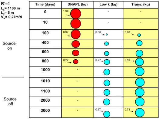
0.37 0.27 0.03 -Low k (kg) -1000 -1010 -1100 -2000 0.71 -3000 0.59 0.22 800 600 400 0.08 0.97 100 -10 -1.08 0 Trans. (kg) DNAPL (kg) Time (days) R`=1 L_x= 1100 m Ly= 5 m Vw= 0.27m/d Source on Source off

Figure 6. Predicted PCE DNAPL and total aqueous PCE mass in transmissive (R=1) and low permeability (R’=1) layers over time

In Figure 6, circles (bubbles) represent the total mass in transmissive and low permeability layers at different times. As DNAPL is depleted, contaminants move from the transmissive layer into the low permeability layer. At the end of the loading with no retardation in the low permeability zone, 32% of the released contaminant is present in the low permeability layer. Even after the source is shut down, contaminant mass in the transmissive layer is growing through inward diffusion from the low permeability layer. 3.1.2 Scenario 2: with adsorption

To take into account the effect of sorption, the retardation coefficient of the low permeability layer is elevated to 10 and Figure 7 and Figure 8 are generated following the same scenario as presented in Figure 5 and Figure 6. The low permeability layer’s

retardation factor is based on a bulk density of 1590 kg/m3_{, f}

oc= 0.006 and Koc= 0.364

mL/g for PCE.

Masses are reported in kilograms per 1 meter width of the porous media. Total masses were calculated from Equations (11a) to (13). Figure 7 illustrates that in the end of loading given a retardation factor of 10 in the low permeability zone, 58% of the released contaminant is present in the low permeability layer versus 32% before. In Figure 8 blue wedges represent aqueous PCE mass and gray represents sorbed PCE mass in the low permeability layer. And again an increase in PCE mass in low permeability layer is observed after source is off due to back diffusion.

0.66 0.49 0.05 -Low k (kg) 0.46 -1000 -1010 -1100 -2000 0.42 -3000 0.37 0.22 800 600 400 0.06 100 -10 -1.08 0 Trans. (kg) DNAPL (kg) Time (days) Source on Source off Sorbed Aq. R`=10 L_x= 1100 m L_y= 5 m Vw= 0.27m/d

Figure 8. The effect of elevating R’ from 1 to 10 on predicted total aqueous and sorbed PCE mass in transmissive(R=1) and low permeability layers.

Figure 7. The effect of elevating R’ from 1 to 10 on total PCE mass in transmissive (R=1) and low permeability layers. 0 0.2 0.4 0.6 0.8 1 1.2 0 500 1000 1500 2000 2500 3000 Time (days) Ma s s ( k g ) Msource(t) Trans.

3.2 Spatial variation in mass in low permeability zones 3.2.1 Scenario 1: without adsorption

Figure 9 illustrates contaminant mass in the low permeability zone in terms of 2

/ ( of contact area of the plume and the low permeability layer)

mg m when no adsorption

occurs in the transmissive and low permeability layers (retardation coefficients of 1). Areas of the circles are proportional to the total mass present at given position and time.

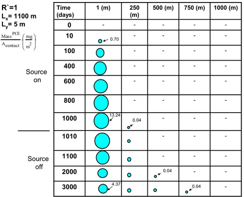
-3000 -2000 -1100 -1010 -1000 -800 -600 -400 -100 -10 -0 1000 (m) 750 (m) 500 (m) 250 (m) 1 (m) Time (days) R`=1 L_x= 1100 m L_y= 5 m 0.70 4.37 13.24 0.04 0.04 0.04 Source on Source off MassPCE Acontact mg m2 ⎛ ⎜ ⎝ ⎞ ⎟ ⎠ ⋅

Figure 9. Spatial distribution of PCE mass in transects of the low permeability layer (R`=1).

As DNAPL gets depleted, contaminants move from the transmissive layer into the low permeability layer. Figure 9 shows that first of all PCE mass is not uniformly

distributed in the soil profile. Second of all, PCE mass is decreasing in source vicinity after the source has been exhausted. Third of all, PCE mass is increasing in the leading edge. Lastly, the domain with significant mass is observed to be located in proximity of the DNAPL release area in the plume. This reflects the fact that, for the scenarios

considered, the domain located in proximity of the DNAPL areas has had contact with the highest contaminant concentrations for the longest period of time. Future work should focus on a more comprehensive analysis of spatial and temporal variations in contaminant storage in low permeability zones after source removal.

3.2.2 Scenario 2: with adsorption

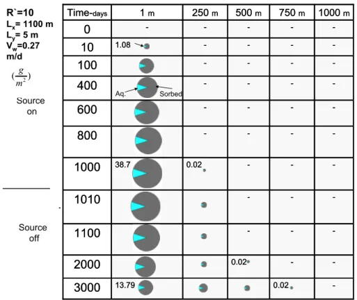
Figure 10 depicts the same scenario as Figure 9 with the modification of retardation factor of the low permeability layer from 1 to 10. In this figure masses are also in grams per square meter of the contact area of the plume and the low permeability layer.

Figure 10. Spatial distribution of PCE mass in transects of the low permeability layer (R`=10).

Fraction of organic carbon of the low permeability layer, octanol-carbon

partitioning coefficient of PCE, and bulk density of the low permeability layer are the same as Section 2.3.1.2. Comparison of Figure 10 with Figure 9 indicates almost 3 times less PCE mass accumulation in the aqueous phase of the low permeability layer when sorption is considered. A key element in Figure 10 is that the contaminants are not uniformly distributed in the low permeability layer. An interesting aspect of this observation is that the need to treat contaminants in low permeability zones may be limited to a subset of the plume domain. Specifically, the majority of the mass remain in vicinity of the DNAPL source.

4. Conclusions

The temporal and spatial evolution of a contaminant release in transmissive and low permeability zones has been examined using analytical solutions. The model addresses a two-layer system involving a transmissive layer (e.g. sand) situated above a low permeability layer (e.g. silt) with a DNAPL like source at the contact of the two layers. The model is based on advective flow through the transmissive layer, transverse diffusion across the transmissive layer, and transverse molecular diffusion in the low permeability layer. Initial efforts focused on conducted calculations using a hybrid method employing a Sale et al. (2008) Mathcad worksheet solution for small distances and series approximation for large distances. While the hybrid approach expanded the domain of accurate

calculation it also failed at large domains. In the end, this analysis relies on using the Sale et al. (2008) solution for the low permeability layer (which is stable for all values of x), an estimate of the total mass in the system from the source, and defining the contaminant

-0.02 13.79 3000 -0.02 2000 -1100 -1010 -0.02 38.7 1000 -800 -600 -400 -100 -1.08 10 -0 1000 m 750 m 500 m 250 m 1 m Time-days -0.02 13.79 3000 -0.02 2000 -1100 -1010 -0.02 38.7 1000 -800 -600 -400 -100 -1.08 10 -0 1000 m 750 m 500 m 250 m 1 m Time-days R`=10 L_x= 1100 m L_y= 5 m V_w=0.27 m/d Source on Source off gm m2 ⎛ ⎜ ⎝ ⎞ ⎟ ⎠ Sorbed Aq. 2 (g ) m

mass in the transmissive layer as the difference between total mass in the system and total mass in the low permeability layer. Efforts to develop practical approaches for the

transmissive layer solution at large domains are ongoing at Colorado State University. Three important observations are developed from this study. First, the hypothesis that chlorinated solvent releases can evolve with time has been validated. Specially, through time, the nature of the problem changed from DNAPL in the transmissive layer to that of aqueous and sorbed contaminants in the low permeability layer. Given that

remedies for DNAPL in transmissive zones and contaminants in low permeability zones can be quite different, an understanding of the age of a release can be an important part of selecting appropriate site remedies and anticipating their performance.

The second major result of this work is that contaminant storage in low permeability zones varies spatially with time. Specially, observed contaminant distributions in the low permeability layer suggest that even at late stages much of the contaminant mass in low permeability zone remains in proximity to the DNAPL source. This leads to the observation that domain in which contaminants are present (at significant levels) in low permeability zones can be a subset of the entire plume domain. An ability to resolve treatment of contaminant in low permeability zones holds promise for more

efficient remedies for chlorinated solvent releases.

Lastly, retardation in the low permeability layer controls contaminants mass stored in the low permeability layer at late time. In the case of R=1 in the low permeability layer, 32% of the released contaminant mass is present in the low permeability layer after 1000 days. In contrast, given R=10 in the low permeability layer, 58% of the released

contaminant mass is present in the low permeability layer after 1000 days. Overall, the low permeability zone retardation factors appear to be an important factor in understanding the nature of the problem posed by late stage chlorinated solvent releases.

Acknowledgements. To be greatly thanked are Dr. David Dandy and Dr. Domenico Bau,

professors at Colorado State University, for their great support and guidelines on different aspects of the modeling. Funding of this research was in part provided by University Consortium for Field-Focused Groundwater Contamination.

References

Al-Niami, A.N.S., Rushton, K.R., 1979. Dispersion in stratified porous media: analytical solutions. Water Resources Research 15, 1044-1048.

Cameron, D.R., Klute, A., 1977. Convective-dispersive solute transport with a combined equilibrium and kinetic adsorption model. Water Resources Research 13, 183-188.

Chapman, S.W., B.L. Parker, 2005. Plume persistence due to aquitard back diffusion following dense

nonaqueous phase liquid removal or isolation, Water Resource Research 41 (12), W12411.

Feenstra, S., Cherry, J.A., Parker, B.L., 1996. Conceptual Models for the Behavior of Dense Nonaqueous Phase Liquids (DNAPLs) in the Subsurface, Chapter 2 in Dense Chlorinated Solvents and Other DNAPLs in Groundwater, J.F Pankow and J.A. Cherry, Editors. Waterloo Press, pp. 53-88. Guyonnet, G., Neville, C., 2004. Dimensionless analysis of two analytical solutions for

3-D solute transport in groundwater. Journal of Contaminant Hydrology 75, 141-153. Kueper, B.H., McWhorter, D.B., 1991. The behavior of dense nonaqueous phase liquids

in fractured clay and rock. Journal of Ground Water 29, 716–728.

Liu, G., Ball, W.P., 2002. Back diffusion of chlorinated solvent contamination from a

natural aquitard to a remediated aquifer under well-controlled field conditions: predictions and measurements, Journal of Ground Water 40, 175-184.

National Research Council (NRC), 2005. Contaminants in the Subsurface: Source Zone

Assessment and Remediation. National Academies Press, Washington, D.C.

Newell, C.J., Hopkins, L.P., Bedient, P.B., 1990. A hydrogeologic database for ground water- modeling. Ground Water 28(5): 703-714.

Parker, B.L., Chapman, S.W., Guilbeault, M.A., 2008. Plume resistence caused by back

diffusion from thin clay layers in a sand aquifer following TCE source-zone hydraulic isolation, Journal of Contaminant Hydrology 102, 72-85.

Parker B.L., Gillham R.W., Cherry J.A., 1994. Diffusive disappearance of

immiscible–phase organic liquids in fractured geologic media. Ground Water 32: 805-820. Sale, T.C., McWhorter, D.B., 2001. Steady state mass transfer from single component

dense nonaqueous phase liquids in uniform flow fields. Water Resources Research 37, 393-404. Sale, T. C., Newell, C., 2011. A Guide for Selecting Remedies for Subsurface Releases of

Chlorinated Solvents, ESTCP Project ER-0530.

Sale, T. C., Zimbron, J., Dandy, D., 2008. Effects of reduced contaminant loading on

downgradient water quality in an idealized two-layer granular porous media, Journal of Contaminant Hydrology 102, 72-85.

Skopp, J., Warrick, A.W., 1974. A two-phase model for the miscible displacement of reactive solutes in soils. Soil Science Society of America Proceedings 38, 545-550. Sudicky E.A., 1986. A natural gradient experiment on solute transport in a sand aquifer:

Spatial variability of hydraulic conductivity and its role in the dispersion process. Water Resources Research 22, 2069-2082.

Sudicky, E.A., Frind, E.O., 1982. Contaminant transport in fractured porous media:

analytical solutions for a system of parallel fractures. Water Resources Research 18, 1634-1642. Tang, D.H., Frind, E.O., Sudicky, E.A., 1981. Contaminant transport in fractured porous

Appendix 1- Summarized equivalent series for: 2 2 2 b x b y e erfc x x φ φ φ ∗ ⎛ ∗ ⎞ ∗ _⎜ ∗ + _⎟ ⎝ ⎠ 1 b φ e 2 − φ y⋅ 2 ⋅ b φ ⋅ 1 x ⋅ π 2 b φ ⎛⎜ ⎝ ⎞⎟⎠ 2 ⋅ φ y⋅ 2 ⎛⎜ ⎝ ⎞⎟⎠ 2 ⋅ 2b φ ⋅ φ y⋅ 2 ⋅ + +1 ⎡ ⎢ ⎣ ⎤ ⎥ ⎦ − e 2 − b φ φ y⋅ 2 ⋅ ⎛⎜ ⎝ ⎞⎟⎠ ⋅ ⋅ 1 x ⎛⎜ ⎝ ⎞⎟⎠ 3 2 ⋅ 2 b φ ⎛⎜ ⎝ ⎞⎟⎠ 2 ⋅ ⋅π + ... 2 b φ ⎛⎜ ⎝ ⎞⎟⎠ 4 ⋅ φ y⋅ 2 ⎛⎜ ⎝ ⎞⎟⎠ 4 ⋅ 4 b φ ⎛⎜ ⎝ ⎞⎟⎠ 3 ⋅ φ y⋅ 2 ⎛⎜ ⎝ ⎞⎟⎠ 3 ⋅ + 6 b φ ⎛⎜ ⎝ ⎞⎟⎠ 2 ⋅ φ y⋅ 2 ⎛⎜ ⎝ ⎞⎟⎠ 2 ⋅ + 6 b φ ⎛⎜ ⎝ ⎞⎟⎠ ⋅ φ y⋅ 2 ⎛⎜ ⎝ ⎞⎟⎠ ⋅ + +3 ⎡ ⎢ ⎣ ⎤ ⎥ ⎦e 2 − b φ φ y⋅ 2 ⋅ ⎛⎜ ⎝ ⎞⎟⎠ ⋅ ⋅ 1 x ⎛⎜ ⎝ ⎞⎟⎠ 5 2 ⋅ 4 b φ ⎛⎜ ⎝ ⎞⎟⎠ 4 ⋅ ⋅π + ... 1 − 4 b φ ⎛⎜ ⎝ ⎞⎟⎠ 6 ⋅ φ y⋅ 2 ⎛⎜ ⎝ ⎞⎟⎠ 6 ⋅ 12 b φ ⎛⎜ ⎝ ⎞⎟⎠ 5 ⋅ φ y⋅ 2 ⎛⎜ ⎝ ⎞⎟⎠ 5 ⋅ + 30 b φ ⎛⎜ ⎝ ⎞⎟⎠ 4 ⋅ φ y⋅ 2 ⎛⎜ ⎝ ⎞⎟⎠ 4 ⋅ + 60 b φ ⎛⎜ ⎝ ⎞⎟⎠ 3 ⋅ φ y⋅ 2 ⎛⎜ ⎝ ⎞⎟⎠ 3 ⋅ + 90 b φ ⎛⎜ ⎝ ⎞⎟⎠ 2 ⋅ φ y⋅ 2 ⎛⎜ ⎝ ⎞⎟⎠ 2 ⋅ + 90 b φ ⎛⎜ ⎝ ⎞⎟⎠ 1 ⋅ φ y⋅ 2 ⎛⎜ ⎝ ⎞⎟⎠ 1 ⋅ + +45 ⎡ ⎢ ⎣ ⎤ ⎥ ⎦ ⋅ e 2 − b φ φ y⋅ 2 ⋅ ⎛⎜ ⎝ ⎞⎟⎠ ⋅ ⋅ 1 x ⎛⎜ ⎝ ⎞⎟⎠ 7 2 ⋅ 24 b φ ⎛⎜ ⎝ ⎞⎟⎠ 6 ⋅ ⋅π + ... 1 2 b φ ⎛⎜ ⎝ ⎞⎟⎠ 8 ⋅ φ y⋅ 2 ⎛⎜ ⎝ ⎞⎟⎠ 8 ⋅ 8 b φ ⎛⎜ ⎝ ⎞⎟⎠ 7 ⋅ φ y⋅ 2 ⎛⎜ ⎝ ⎞⎟⎠ 7 ⋅ + 28 b φ ⎛⎜ ⎝ ⎞⎟⎠ 6 ⋅ φ y⋅ 2 ⎛⎜ ⎝ ⎞⎟⎠ 6 ⋅ + 84 b φ ⎛⎜ ⎝ ⎞⎟⎠ 5 ⋅ φ y⋅ 2 ⎛⎜ ⎝ ⎞⎟⎠ 5 ⋅ + 210 b φ ⎛⎜ ⎝ ⎞⎟⎠ 4 ⋅ φ y⋅ 2 ⎛⎜ ⎝ ⎞⎟⎠ 4 ⋅ + 420 b φ ⎛⎜ ⎝ ⎞⎟⎠ 3 ⋅ φ y⋅ 2 ⎛⎜ ⎝ ⎞⎟⎠ 3 ⋅ + 630 b φ ⎛⎜ ⎝ ⎞⎟⎠ 2 ⋅ φ y⋅ 2 ⎛⎜ ⎝ ⎞⎟⎠ 2 ⋅ + 630 b φ ⎛⎜ ⎝ ⎞⎟⎠ 1 ⋅ φ y⋅ 2 ⎛⎜ ⎝ ⎞⎟⎠ 1 ⋅ + +315 ⎡ ⎢ ⎣ ⎤ ⎥ ⎦ ⋅ e 2 − b φ φ y⋅ 2 ⋅ ⎛⎜ ⎝ ⎞⎟⎠ ⋅ ⋅ 1 x ⎛⎜ ⎝ ⎞⎟⎠ 9 2 ⋅ 48 b φ ⎛⎜ ⎝ ⎞⎟⎠ 8 ⋅ ⋅π + ... b φ 1 x ⎛⎜ ⎝ ⎞⎟⎠ 11 2 ⋅ e 2 − b φ φ y⋅ 2 ⋅ ⎛⎜ ⎝ ⎞⎟⎠ ⋅ − φ y⋅ 2 ⎛⎜ ⎝ ⎞⎟⎠ 10 120b φ ⋅ ⋅π ⋅ φ y⋅ 2 − b φ ⎛⎜ ⎝ ⎞⎟⎠ 2 1 2 b φ ⎛⎜ ⎝ ⎞⎟⎠ 3 ⋅ − ⎡⎢ ⎢ ⎢ ⎢⎣ ⎤⎥ ⎥ ⎥ ⎥⎦ e 2 − b φ φ y⋅ 2 ⋅ ⎛⎜ ⎝ ⎞⎟⎠ ⋅ ⋅ φ y⋅ 2 ⎛⎜ ⎝ ⎞⎟⎠ 8 ⋅ 24⋅ π + φ y⋅ 2 ⎛⎜ ⎝ ⎞⎟⎠ 2 b φ ⎛⎜ ⎝ ⎞⎟⎠ 3 φ y⋅ 2 2 b φ ⎛⎜ ⎝ ⎞⎟⎠ 4 ⋅ + φ y⋅ 2 b φ ⎛⎜ ⎝ ⎞⎟⎠ 3 3 4 b φ ⎛⎜ ⎝ ⎞⎟⎠ 4 ⋅ + b φ + ⎡⎢ ⎢ ⎢ ⎢ ⎢ ⎢ ⎢⎣ ⎤⎥ ⎥ ⎥ ⎥ ⎥ ⎥ ⎥⎦ − e 2 − b φ φ y⋅ 2 ⋅ ⎛⎜ ⎝ ⎞⎟⎠ ⋅ ⋅ φ y⋅ 2 ⎛⎜ ⎝ ⎞⎟⎠ 6 ⋅ 6⋅π ( ) + ... φ y⋅ 2 ⎛⎜ ⎝ ⎞⎟⎠ 3 b φ ⎛⎜ ⎝ ⎞⎟⎠ 4 − φ y⋅ 2 ⎛⎜ ⎝ ⎞⎟⎠ 2 − 2 b φ ⎛⎜ ⎝ ⎞⎟⎠ 5 ⋅ + φ y⋅ 2 b φ ⎛⎜ ⎝ ⎞⎟⎠ 3 3 4 b φ ⎛⎜ ⎝ ⎞⎟⎠ 4 ⋅ + ⎡⎢ ⎢ ⎢ ⎢⎣ ⎤⎥ ⎥ ⎥ ⎥⎦ φ y⋅ 2 ⋅ b φ ⎛⎜ ⎝ ⎞⎟⎠ 2 − 3 − φ y⋅ 2 ⎛⎜ ⎝ ⎞⎟⎠ 2 ⋅ 2 b φ ⎛⎜ ⎝ ⎞⎟⎠ 4 ⋅ 3φ y⋅ 2 ⋅ b φ ⎛⎜ ⎝ ⎞⎟⎠ 5 − 15 8 b φ ⎛⎜ ⎝ ⎞⎟⎠ 6 ⋅ − b φ + ⎡ ⎢ ⎢ ⎢ ⎢ ⎢ ⎢ ⎢ ⎣ ⎤ ⎥ ⎥ ⎥ ⎥ ⎥ ⎥ ⎥ ⎦ e 2 − b φ φ y⋅ 2 ⋅ ⎛⎜ ⎝ ⎞⎟⎠ ⋅ ⋅ φ y⋅ 2 ⎛⎜ ⎝ ⎞⎟⎠ 4 ⋅ 2⋅ π + ... 1 − πe 2 − b φ φ y⋅ 2 ⋅ ⎛⎜ ⎝ ⎞⎟⎠ ⋅ ⋅ φ y⋅ 2 ⎛⎜ ⎝ ⎞⎟⎠ 2 ⋅ φ y⋅ 2 ⎛⎜ ⎝ ⎞⎟⎠ 4 b φ ⎛⎜ ⎝ ⎞⎟⎠ 5 φ y⋅ 2 ⎛⎜ ⎝ ⎞⎟⎠ 3 2 b φ ⎛⎜ ⎝ ⎞⎟⎠ 6 ⋅ + φ y⋅ 2 b φ ⎛⎜ ⎝ ⎞⎟⎠ 3 3 4 b φ ⎛⎜ ⎝ ⎞⎟⎠ 4 ⋅ + ⎡⎢ ⎢ ⎢ ⎢⎣ ⎤⎥ ⎥ ⎥ ⎥⎦ φ y⋅ 2 ⎛⎜ ⎝ ⎞⎟⎠ 2 ⋅ b φ ⎛⎜ ⎝ ⎞⎟⎠ 3 + 3 − φ y⋅ 2 ⎛⎜ ⎝ ⎞⎟⎠ 2 ⋅ 2 b φ ⎛⎜ ⎝ ⎞⎟⎠ 4 ⋅ 3φ y⋅ 2 ⋅ b φ ⎛⎜ ⎝ ⎞⎟⎠ 5 − 15 8 b φ ⎛⎜ ⎝ ⎞⎟⎠ 6 ⋅ − ⎡ ⎢ ⎢ ⎢ ⎢ ⎣ ⎤ ⎥ ⎥ ⎥ ⎥ ⎦ − φ y⋅ 2 ⋅ b φ ⎛⎜ ⎝ ⎞⎟⎠ 2 2 φ y⋅ 2 ⎛⎜ ⎝ ⎞⎟⎠ 3 ⋅ b φ ⎛⎜ ⎝ ⎞⎟⎠ 5 15 φ y⋅ 2 ⎛⎜ ⎝ ⎞⎟⎠ 2 ⋅ b φ ⎛⎜ ⎝ ⎞⎟⎠ 6 2 ⋅ + 45φ y⋅ 2 ⋅ 4 b φ ⎛⎜ ⎝ ⎞⎟⎠ 7 ⋅ + 105 16 b φ ⎛⎜ ⎝ ⎞⎟⎠ 8 ⋅ + b φ ⎛⎜ ⎝ ⎞⎟⎠ 1 + + ... ⎡ ⎢ ⎢ ⎢ ⎢ ⎢ ⎢ ⎢ ⎢ ⎢ ⎢ ⎢ ⎢ ⎢ ⎢ ⎢ ⎣ ⎤ ⎥ ⎥ ⎥ ⎥ ⎥ ⎥ ⎥ ⎥ ⎥ ⎥ ⎥ ⎥ ⎥ ⎥ ⎥ ⎦ ⋅ + ... 1 πe 2 − b φ φ y⋅ 2 ⋅ ⎛⎜ ⎝ ⎞⎟⎠ ⋅ ⋅ φ y⋅ 2 ⎛⎜ ⎝ ⎞⎟⎠ 5 − b φ ⎛⎜ ⎝ ⎞⎟⎠ 6 φ y⋅ 2 ⎛⎜ ⎝ ⎞⎟⎠ 4 2 b φ ⎛⎜ ⎝ ⎞⎟⎠ 7 ⋅ − φ y⋅ 2 b φ ⎛⎜ ⎝ ⎞⎟⎠ 3 3 4 b φ ⎛⎜ ⎝ ⎞⎟⎠ 4 ⋅ + ⎡⎢ ⎢ ⎢ ⎢⎣ ⎤⎥ ⎥ ⎥ ⎥⎦ φ y⋅ 2 ⎛⎜ ⎝ ⎞⎟⎠ 3 ⋅ b φ ⎛⎜ ⎝ ⎞⎟⎠ 4 − 3 − φ y⋅ 2 ⎛⎜ ⎝ ⎞⎟⎠ 2 2 b φ ⎛⎜ ⎝ ⎞⎟⎠ 4 ⋅ 3 − φ y⋅ 2 ⋅ b φ ⎛⎜ ⎝ ⎞⎟⎠ 5 + 15 8 b φ ⎛⎜ ⎝ ⎞⎟⎠ 6 ⋅ − ⎡ ⎢ ⎢ ⎢ ⎢ ⎣ ⎤ ⎥ ⎥ ⎥ ⎥ ⎦ φ y⋅ 2 ⎛⎜ ⎝ ⎞⎟⎠ 2 ⋅ b φ ⎛⎜ ⎝ ⎞⎟⎠ 3 + 2 φ y⋅ 2 ⎛⎜ ⎝ ⎞⎟⎠ 3 b φ ⎛⎜ ⎝ ⎞⎟⎠ 5 15 φ y⋅ 2 ⎛⎜ ⎝ ⎞⎟⎠ 2 ⋅ b φ ⎛⎜ ⎝ ⎞⎟⎠ 6 2 ⋅ + 45φ y⋅ 2 ⋅ 4 b φ ⎛⎜ ⎝ ⎞⎟⎠ 7 ⋅ + 105 16 b φ ⎛⎜ ⎝ ⎞⎟⎠ 8 ⋅ + ⎡ ⎢ ⎢ ⎢ ⎢ ⎣ ⎤ ⎥ ⎥ ⎥ ⎥ ⎦ − φ y⋅ 2 ⎛⎜ ⎝ ⎞⎟⎠ 1 ⋅ b φ ⎛⎜ ⎝ ⎞⎟⎠ 2 + ... 5 − φ y⋅ 2 ⎛⎜ ⎝ ⎞⎟⎠ 4 2 b φ ⎛⎜ ⎝ ⎞⎟⎠ 6 15 − φ y⋅ 2 ⎛⎜ ⎝ ⎞⎟⎠ 3 ⋅ b φ ⎛⎜ ⎝ ⎞⎟⎠ 7 + 315 − φ y⋅ 2 ⎛⎜ ⎝ ⎞⎟⎠ 2 ⋅ 8 b φ ⎛⎜ ⎝ ⎞⎟⎠ 8 ⋅ + 105 − φ y⋅ 2 ⋅ 2 b φ ⎛⎜ ⎝ ⎞⎟⎠ 9 ⋅ + 945 32 b φ ⎛⎜ ⎝ ⎞⎟⎠ 10 ⋅ − b ⎛⎜ ⎝ ⎞⎟⎠ + ... ⎡ ⎢ ⎢ ⎢ ⎢ ⎢ ⎢ ⎢ ⎢ ⎢ ⎢ ⎢ ⎢ ⎢ ⎢ ⎢ ⎢ ⎢ ⎢ ⎢ ⎢ ⎢ ⎢ ⎢ ⎢ ⎣ ⎤ ⎥ ⎥ ⎥ ⎥ ⎥ ⎥ ⎥ ⎥ ⎥ ⎥ ⎥ ⎥ ⎥ ⎥ ⎥ ⎥ ⎥ ⎥ ⎥ ⎥ ⎥ ⎥ ⎥ ⎥ ⎦ ⋅ + ... ⎡ ⎢ ⎢ ⎢ ⎢ ⎢ ⎢ ⎢ ⎢ ⎢ ⎢ ⎢ ⎢ ⎢ ⎢ ⎢ ⎢ ⎢ ⎢ ⎢ ⎢ ⎢ ⎢ ⎢ ⎢ ⎢ ⎢ ⎢ ⎢ ⎢ ⎢ ⎢ ⎢ ⎢ ⎢ ⎢ ⎢ ⎢ ⎢ ⎢ ⎢ ⎢ ⎢ ⎢ ⎢ ⎢ ⎢ ⎢ ⎢ ⎢ ⎢ ⎢ ⎢ ⎢ ⎢ ⎢ ⎢ ⎢ ⎢ ⎢ ⎢ ⎢ ⎢ ⎢ ⎢ ⎢ ⎢ ⎢ ⎢ ⎣ ⎤ ⎥ ⎥ ⎥ ⎥ ⎥ ⎥ ⎥ ⎥ ⎥ ⎥ ⎥ ⎥ ⎥ ⎥ ⎥ ⎥ ⎥ ⎥ ⎥ ⎥ ⎥ ⎥ ⎥ ⎥ ⎥ ⎥ ⎥ ⎥ ⎥ ⎥ ⎥ ⎥ ⎥ ⎥ ⎥ ⎥ ⎥ ⎥ ⎥ ⎥ ⎥ ⎥ ⎥ ⎥ ⎥ ⎥ ⎥ ⎥ ⎥ ⎥ ⎥ ⎥ ⎥ ⎥ ⎥ ⎥ ⎥ ⎥ ⎥ ⎥ ⎥ ⎥ ⎥ ⎥ ⎥ ⎥ ⎥ ⎥ ⎦ ⋅ + ... ⎡⎢ ⎢ ⎢ ⎢ ⎢ ⎢ ⎢ ⎢ ⎢ ⎢ ⎢ ⎢ ⎢ ⎢ ⎢ ⎢ ⎢ ⎢ ⎢ ⎢ ⎢ ⎢ ⎢ ⎢ ⎢ ⎢ ⎢ ⎢ ⎢ ⎢ ⎢ ⎢ ⎢ ⎢ ⎢ ⎢ ⎢ ⎢ ⎢ ⎢ ⎢ ⎢ ⎢ ⎢ ⎢ ⎢ ⎢ ⎢ ⎢ ⎢ ⎢ ⎢ ⎢ ⎢ ⎢ ⎢ ⎢ ⎢ ⎢ ⎢ ⎢ ⎢ ⎢ ⎢ ⎢ ⎢ ⎢ ⎢ ⎢ ⎢ ⎢ ⎢ ⎢ ⎢ ⎢ ⎢ ⎢ ⎢ ⎢ ⎢ ⎢ ⎢ ⎢ ⎢ ⎢ ⎢ ⎢ ⎢ ⎢ ⎢ ⎢ ⎢ ⎢ ⎢ ⎢ ⎢ ⎢ ⎢ ⎢ ⎢ ⎢ ⎣ ⎤⎥ ⎥ ⎥ ⎥ ⎥ ⎥ ⎥ ⎥ ⎥ ⎥ ⎥ ⎥ ⎥ ⎥ ⎥ ⎥ ⎥ ⎥ ⎥ ⎥ ⎥ ⎥ ⎥ ⎥ ⎥ ⎥ ⎥ ⎥ ⎥ ⎥ ⎥ ⎥ ⎥ ⎥ ⎥ ⎥ ⎥ ⎥ ⎥ ⎥ ⎥ ⎥ ⎥ ⎥ ⎥ ⎥ ⎥ ⎥ ⎥ ⎥ ⎥ ⎥ ⎥ ⎥ ⎥ ⎥ ⎥ ⎥ ⎥ ⎥ ⎥ ⎥ ⎥ ⎥ ⎥ ⎥ ⎥ ⎥ ⎥ ⎥ ⎥ ⎥ ⎥ ⎥ ⎥ ⎥ ⎥ ⎥ ⎥ ⎥ ⎥ ⎥ ⎥ ⎥ ⎥ ⎥ ⎥ ⎥ ⎥ ⎥ ⎥ ⎥ ⎥ ⎥ ⎥ ⎥ ⎥ ⎥ ⎥ ⎥ ⎥ ⎦ ⋅

Appendix 2- Summarized equivalent series for 2

(

(

)

)

2 1 2 bx b y e erf x x φ φ φ − + + : 1 b φ e 2φ y⋅ 2 ⋅ b φ ⋅ 1 x ⋅ π 2 b φ ⎛⎜ ⎝ ⎞⎟⎠ 2 ⋅ φ y⋅ 2 ⎛⎜ ⎝ ⎞⎟⎠ 2 ⋅ 2b φ ⋅ φ y⋅ 2 ⋅ − +1 ⎡ ⎢ ⎣ ⎤ ⎥ ⎦ − e 2 b φ φ y⋅ 2 ⋅ ⎛⎜ ⎝ ⎞⎟⎠ ⋅ ⋅ 1 x ⎛⎜ ⎝ ⎞⎟⎠ 3 2 ⋅ 2 b φ ⎛⎜ ⎝ ⎞⎟⎠ 2 ⋅ ⋅π + ... 2 b φ ⎛⎜ ⎝ ⎞⎟⎠ 4 ⋅ φ y⋅ 2 ⎛⎜ ⎝ ⎞⎟⎠ 4 ⋅ 4 b φ ⎛⎜ ⎝ ⎞⎟⎠ 3 ⋅ φ y⋅ 2 ⎛⎜ ⎝ ⎞⎟⎠ 3 ⋅ − 6 b φ ⎛⎜ ⎝ ⎞⎟⎠ 2 ⋅ φ y⋅ 2 ⎛⎜ ⎝ ⎞⎟⎠ 2 ⋅ + 6 b φ ⎛⎜ ⎝ ⎞⎟⎠ ⋅ φ y⋅ 2 ⎛⎜ ⎝ ⎞⎟⎠ ⋅ − +3 ⎡ ⎢ ⎣ ⎤ ⎥ ⎦e 2 b φ φ y⋅ 2 ⋅ ⎛⎜ ⎝ ⎞⎟⎠ ⋅ ⋅ 1 x ⎛⎜ ⎝ ⎞⎟⎠ 5 2 ⋅ 4 b φ ⎛⎜ ⎝ ⎞⎟⎠ 4 ⋅ ⋅π + ... 1 − 4 b φ ⎛⎜ ⎝ ⎞⎟⎠ 6 ⋅ φ y⋅ 2 ⎛⎜ ⎝ ⎞⎟⎠ 6 ⋅ 12 b φ ⎛⎜ ⎝ ⎞⎟⎠ 5 ⋅ φ y⋅ 2 ⎛⎜ ⎝ ⎞⎟⎠ 5 ⋅ − 30 b φ ⎛⎜ ⎝ ⎞⎟⎠ 4 ⋅ φ y⋅ 2 ⎛⎜ ⎝ ⎞⎟⎠ 4 ⋅ + 60 b φ ⎛⎜ ⎝ ⎞⎟⎠ 3 ⋅ φ y⋅ 2 ⎛⎜ ⎝ ⎞⎟⎠ 3 ⋅ − 90 b φ ⎛⎜ ⎝ ⎞⎟⎠ 2 ⋅ φ y⋅ 2 ⎛⎜ ⎝ ⎞⎟⎠ 2 ⋅ + 90 b φ ⎛⎜ ⎝ ⎞⎟⎠ 1 ⋅ φ y⋅ 2 ⎛⎜ ⎝ ⎞⎟⎠ 1 ⋅ − +45 ⎡ ⎢ ⎣ ⎤ ⎥ ⎦ ⋅ e 2 b φ φ y⋅ 2 ⋅ ⎛⎜ ⎝ ⎞⎟⎠ ⋅ ⋅ 1 x ⎛⎜ ⎝ ⎞⎟⎠ 7 2 ⋅ 24 b φ ⎛⎜ ⎝ ⎞⎟⎠ 6 ⋅ ⋅π + ... 1 2 b φ ⎛⎜ ⎝ ⎞⎟⎠ 8 ⋅ φ y⋅ 2 ⎛⎜ ⎝ ⎞⎟⎠ 8 ⋅ 8 b φ ⎛⎜ ⎝ ⎞⎟⎠ 7 ⋅ φ y⋅ 2 ⎛⎜ ⎝ ⎞⎟⎠ 7 ⋅ − 28 b φ ⎛⎜ ⎝ ⎞⎟⎠ 6 ⋅ φ y⋅ 2 ⎛⎜ ⎝ ⎞⎟⎠ 6 ⋅ + 84 b φ ⎛⎜ ⎝ ⎞⎟⎠ 5 ⋅ φ y⋅ 2 ⎛⎜ ⎝ ⎞⎟⎠ 5 ⋅ − 210 b φ ⎛⎜ ⎝ ⎞⎟⎠ 4 ⋅ φ y⋅ 2 ⎛⎜ ⎝ ⎞⎟⎠ 4 ⋅ + 420 b φ ⎛⎜ ⎝ ⎞⎟⎠ 3 ⋅ φ y⋅ 2 ⎛⎜ ⎝ ⎞⎟⎠ 3 ⋅ − 630 b φ ⎛⎜ ⎝ ⎞⎟⎠ 2 ⋅ φ y⋅ 2 ⎛⎜ ⎝ ⎞⎟⎠ 2 ⋅ + 630 b φ ⎛⎜ ⎝ ⎞⎟⎠ 1 ⋅ φ y⋅ 2 ⎛⎜ ⎝ ⎞⎟⎠ 1 ⋅ − +315 ⎡ ⎢ ⎣ ⎤ ⎥ ⎦ ⋅ e 2 b φ φ y⋅ 2 ⋅ ⎛⎜ ⎝ ⎞⎟⎠ ⋅ ⋅ 1 x ⎛⎜ ⎝ ⎞⎟⎠ 9 2 ⋅ 48 b φ ⎛⎜ ⎝ ⎞⎟⎠ 8 ⋅ ⋅ π + ... b φ 1 x ⎛⎜ ⎝ ⎞⎟⎠ 11 2 ⋅ e 2 b φ φ y⋅ 2 ⋅ ⎛⎜ ⎝ ⎞⎟⎠ ⋅ − φ y⋅ 2 ⎛⎜ ⎝ ⎞⎟⎠ 10 120b φ ⋅ ⋅π ⋅ φ y⋅ 2 b φ ⎛⎜ ⎝ ⎞⎟⎠ 2 1 2 b φ ⎛⎜ ⎝ ⎞⎟⎠ 3 ⋅ − ⎡⎢ ⎢ ⎢ ⎢⎣ ⎤⎥ ⎥ ⎥ ⎥⎦ e 2 b φ φ y⋅ 2 ⋅ ⎛⎜ ⎝ ⎞⎟⎠ ⋅ ⋅ φ y⋅ 2 ⎛⎜ ⎝ ⎞⎟⎠ 8 ⋅ 24⋅ π + φ y⋅ 2 ⎛⎜ ⎝ ⎞⎟⎠ 2 b φ ⎛⎜ ⎝ ⎞⎟⎠ 3 φ y⋅ 2 2 b φ ⎛⎜ ⎝ ⎞⎟⎠ 4 ⋅ − φ − ⋅y 2 b φ ⎛⎜ ⎝ ⎞⎟⎠ 3 3 4 b φ ⎛⎜ ⎝ ⎞⎟⎠ 4 ⋅ + b φ + ⎡⎢ ⎢ ⎢ ⎢ ⎢ ⎢ ⎢⎣ ⎤⎥ ⎥ ⎥ ⎥ ⎥ ⎥ ⎥⎦ − e 2 b φ φ y⋅ 2 ⋅ ⎛⎜ ⎝ ⎞⎟⎠ ⋅ ⋅ φ y⋅ 2 ⎛⎜ ⎝ ⎞⎟⎠ 6 ⋅ 6⋅ π ( ) + ... φ y⋅ 2 ⎛⎜ ⎝ ⎞⎟⎠ 3 b φ ⎛⎜ ⎝ ⎞⎟⎠ 4 φ y⋅ 2 ⎛⎜ ⎝ ⎞⎟⎠ 2 − 2 b φ ⎛⎜ ⎝ ⎞⎟⎠ 5 ⋅ + ⎡ ⎢ ⎢ ⎢ ⎢ ⎣ ⎤ ⎥ ⎥ ⎥ ⎥ ⎦ φ − ⋅y 2 b φ ⎛⎜ ⎝ ⎞⎟⎠ 3 3 4 b φ ⎛⎜ ⎝ ⎞⎟⎠ 4 ⋅ + ⎡⎢ ⎢ ⎢ ⎢⎣ ⎤⎥ ⎥ ⎥ ⎥⎦ φ y⋅ 2 ⋅ b φ ⎛⎜ ⎝ ⎞⎟⎠ 2 + 3 − φ y⋅ 2 ⎛⎜ ⎝ ⎞⎟⎠ 2 ⋅ 2 b φ ⎛⎜ ⎝ ⎞⎟⎠ 4 ⋅ 3φ y⋅ 2 ⋅ b φ ⎛⎜ ⎝ ⎞⎟⎠ 5 + 15 8 b φ ⎛⎜ ⎝ ⎞⎟⎠ 6 ⋅ − b φ + ⎡ ⎢ ⎢ ⎢ ⎢ ⎢ ⎢ ⎢ ⎣ ⎤ ⎥ ⎥ ⎥ ⎥ ⎥ ⎥ ⎥ ⎦ e 2 − b φ φ y⋅ 2 ⋅ ⎛⎜ ⎝ ⎞⎟⎠ ⋅ ⋅ φ y⋅ 2 ⎛⎜ ⎝ ⎞⎟⎠ 4 ⋅ 2⋅π + ... 1 − πe 2 b φ φ y⋅ 2 ⋅ ⎛⎜ ⎝ ⎞⎟⎠ ⋅ ⋅ φ y⋅ 2 ⎛⎜ ⎝ ⎞⎟⎠ 2 ⋅ φ y⋅ 2 ⎛⎜ ⎝ ⎞⎟⎠ 4 b φ ⎛⎜ ⎝ ⎞⎟⎠ 5 φ y⋅ 2 ⎛⎜ ⎝ ⎞⎟⎠ 3 2 b φ ⎛⎜ ⎝ ⎞⎟⎠ 6 ⋅ − φ − ⋅y 2 b φ ⎛⎜ ⎝ ⎞⎟⎠ 3 3 4 b φ ⎛⎜ ⎝ ⎞⎟⎠ 4 ⋅ + ⎡⎢ ⎢ ⎢ ⎢⎣ ⎤⎥ ⎥ ⎥ ⎥⎦ φ y⋅ 2 ⎛⎜ ⎝ ⎞⎟⎠ 2 ⋅ b φ ⎛⎜ ⎝ ⎞⎟⎠ 3 + 3 − φ y⋅ 2 ⎛⎜ ⎝ ⎞⎟⎠ 2 ⋅ 2 b φ ⎛⎜ ⎝ ⎞⎟⎠ 4 ⋅ 3φ y⋅ 2 ⋅ b φ ⎛⎜ ⎝ ⎞⎟⎠ 5 + 15 8 b φ ⎛⎜ ⎝ ⎞⎟⎠ 6 ⋅ − ⎡ ⎢ ⎢ ⎢ ⎢ ⎣ ⎤ ⎥ ⎥ ⎥ ⎥ ⎦ φ y⋅ 2 ⋅ b φ ⎛⎜ ⎝ ⎞⎟⎠ 2 2 − φ y⋅ 2 ⎛⎜ ⎝ ⎞⎟⎠ 3 ⋅ b φ ⎛⎜ ⎝ ⎞⎟⎠ 5 15 φ y⋅ 2 ⎛⎜ ⎝ ⎞⎟⎠ 2 ⋅ b φ ⎛⎜ ⎝ ⎞⎟⎠ 6 2 ⋅ + 45φ y⋅ 2 ⋅ 4 b φ ⎛⎜ ⎝ ⎞⎟⎠ 7 ⋅ − 105 16 b φ ⎛⎜ ⎝ ⎞⎟⎠ 8 ⋅ + b φ ⎛⎜ ⎝ ⎞⎟⎠ 1 + + ... ⎡ ⎢ ⎢ ⎢ ⎢ ⎢ ⎢ ⎢ ⎢ ⎢ ⎢ ⎢ ⎢ ⎢ ⎢ ⎢ ⎣ ⎤ ⎥ ⎥ ⎥ ⎥ ⎥ ⎥ ⎥ ⎥ ⎥ ⎥ ⎥ ⎥ ⎥ ⎥ ⎥ ⎦ ⋅ + ... 1 πe 2 b φ φ y⋅ 2 ⋅ ⎛⎜ ⎝ ⎞⎟⎠ ⋅ ⋅ φ y⋅ 2 ⎛⎜ ⎝ ⎞⎟⎠ 5 b φ ⎛⎜ ⎝ ⎞⎟⎠ 6 φ y⋅ 2 ⎛⎜ ⎝ ⎞⎟⎠ 4 2 b φ ⎛⎜ ⎝ ⎞⎟⎠ 7 ⋅ − φ − ⋅y 2 b φ ⎛⎜ ⎝ ⎞⎟⎠ 3 3 4 b φ ⎛⎜ ⎝ ⎞⎟⎠ 4 ⋅ + ⎡⎢ ⎢ ⎢ ⎢⎣ ⎤⎥ ⎥ ⎥ ⎥⎦ φ y⋅ 2 ⎛⎜ ⎝ ⎞⎟⎠ 3 ⋅ b φ ⎛⎜ ⎝ ⎞⎟⎠ 4 + 3 − φ y⋅ 2 ⎛⎜ ⎝ ⎞⎟⎠ 2 2 b φ ⎛⎜ ⎝ ⎞⎟⎠ 4 ⋅ 3φ y⋅ 2 ⋅ b φ ⎛⎜ ⎝ ⎞⎟⎠ 5 + 15 8 b φ ⎛⎜ ⎝ ⎞⎟⎠ 6 ⋅ − ⎡ ⎢ ⎢ ⎢ ⎢ ⎣ ⎤ ⎥ ⎥ ⎥ ⎥ ⎦ φ y⋅ 2 ⎛⎜ ⎝ ⎞⎟⎠ 2 ⋅ b φ ⎛⎜ ⎝ ⎞⎟⎠ 3 + 2 − φ y⋅ 2 ⎛⎜ ⎝ ⎞⎟⎠ 3 b φ ⎛⎜ ⎝ ⎞⎟⎠ 5 15 φ y⋅ 2 ⎛⎜ ⎝ ⎞⎟⎠ 2 ⋅ b φ ⎛⎜ ⎝ ⎞⎟⎠ 6 2 ⋅ + 45φ y⋅ 2 ⋅ 4 b φ ⎛⎜ ⎝ ⎞⎟⎠ 7 ⋅ − 105 16 b φ ⎛⎜ ⎝ ⎞⎟⎠ 8 ⋅ + ⎡ ⎢ ⎢ ⎢ ⎢ ⎣ ⎤ ⎥ ⎥ ⎥ ⎥ ⎦ φ y⋅ 2 ⎛⎜ ⎝ ⎞⎟⎠ 1 ⋅ b φ ⎛⎜ ⎝ ⎞⎟⎠ 2 + ... 5 − φ y⋅ 2 ⎛⎜ ⎝ ⎞⎟⎠ 4 2 b φ ⎛⎜ ⎝ ⎞⎟⎠ 6 15 φ y⋅ 2 ⎛⎜ ⎝ ⎞⎟⎠ 3 ⋅ b φ ⎛⎜ ⎝ ⎞⎟⎠ 7 + 315 − φ y⋅ 2 ⎛⎜ ⎝ ⎞⎟⎠ 2 ⋅ 8 b φ ⎛⎜ ⎝ ⎞⎟⎠ 8 ⋅ + 105φ y⋅ 2 ⋅ 2 b φ ⎛⎜ ⎝ ⎞⎟⎠ 9 ⋅ + 945 32 b φ ⎛⎜ ⎝ ⎞⎟⎠ 10 ⋅ − b φ ⎛⎜ ⎝ ⎞⎟⎠ + ... ⎡ ⎢ ⎢ ⎢ ⎢ ⎢ ⎢ ⎢ ⎢ ⎢ ⎢ ⎢ ⎢ ⎢ ⎢ ⎢ ⎢ ⎢ ⎢ ⎢ ⎢ ⎢ ⎢ ⎢ ⎢ ⎣ ⎤ ⎥ ⎥ ⎥ ⎥ ⎥ ⎥ ⎥ ⎥ ⎥ ⎥ ⎥ ⎥ ⎥ ⎥ ⎥ ⎥ ⎥ ⎥ ⎥ ⎥ ⎥ ⎥ ⎥ ⎥ ⎦ ⋅ + ... ⎡ ⎢ ⎢ ⎢ ⎢ ⎢ ⎢ ⎢ ⎢ ⎢ ⎢ ⎢ ⎢ ⎢ ⎢ ⎢ ⎢ ⎢ ⎢ ⎢ ⎢ ⎢ ⎢ ⎢ ⎢ ⎢ ⎢ ⎢ ⎢ ⎢ ⎢ ⎢ ⎢ ⎢ ⎢ ⎢ ⎢ ⎢ ⎢ ⎢ ⎢ ⎢ ⎢ ⎢ ⎢ ⎢ ⎢ ⎢ ⎢ ⎢ ⎢ ⎢ ⎢ ⎢ ⎢ ⎢ ⎢ ⎢ ⎢ ⎢ ⎢ ⎢ ⎢ ⎢ ⎢ ⎢ ⎢ ⎢ ⎢ ⎣ ⎤ ⎥ ⎥ ⎥ ⎥ ⎥ ⎥ ⎥ ⎥ ⎥ ⎥ ⎥ ⎥ ⎥ ⎥ ⎥ ⎥ ⎥ ⎥ ⎥ ⎥ ⎥ ⎥ ⎥ ⎥ ⎥ ⎥ ⎥ ⎥ ⎥ ⎥ ⎥ ⎥ ⎥ ⎥ ⎥ ⎥ ⎥ ⎥ ⎥ ⎥ ⎥ ⎥ ⎥ ⎥ ⎥ ⎥ ⎥ ⎥ ⎥ ⎥ ⎥ ⎥ ⎥ ⎥ ⎥ ⎥ ⎥ ⎥ ⎥ ⎥ ⎥ ⎥ ⎥ ⎥ ⎥ ⎥ ⎥ ⎥ ⎦ ⋅ + ... ⎡⎢ ⎢ ⎢ ⎢ ⎢ ⎢ ⎢ ⎢ ⎢ ⎢ ⎢ ⎢ ⎢ ⎢ ⎢ ⎢ ⎢ ⎢ ⎢ ⎢ ⎢ ⎢ ⎢ ⎢ ⎢ ⎢ ⎢ ⎢ ⎢ ⎢ ⎢ ⎢ ⎢ ⎢ ⎢ ⎢ ⎢ ⎢ ⎢ ⎢ ⎢ ⎢ ⎢ ⎢ ⎢ ⎢ ⎢ ⎢ ⎢ ⎢ ⎢ ⎢ ⎢ ⎢ ⎢ ⎢ ⎢ ⎢ ⎢ ⎢ ⎢ ⎢ ⎢ ⎢ ⎢ ⎢ ⎢ ⎢ ⎢ ⎢ ⎢ ⎢ ⎢ ⎢ ⎢ ⎢ ⎢ ⎢ ⎢ ⎢ ⎢ ⎢ ⎢ ⎢ ⎢ ⎢ ⎢ ⎢ ⎢ ⎢ ⎢ ⎢ ⎢ ⎢ ⎢ ⎢ ⎢ ⎢ ⎢ ⎢ ⎢ ⎣ ⎤⎥ ⎥ ⎥ ⎥ ⎥ ⎥ ⎥ ⎥ ⎥ ⎥ ⎥ ⎥ ⎥ ⎥ ⎥ ⎥ ⎥ ⎥ ⎥ ⎥ ⎥ ⎥ ⎥ ⎥ ⎥ ⎥ ⎥ ⎥ ⎥ ⎥ ⎥ ⎥ ⎥ ⎥ ⎥ ⎥ ⎥ ⎥ ⎥ ⎥ ⎥ ⎥ ⎥ ⎥ ⎥ ⎥ ⎥ ⎥ ⎥ ⎥ ⎥ ⎥ ⎥ ⎥ ⎥ ⎥ ⎥ ⎥ ⎥ ⎥ ⎥ ⎥ ⎥ ⎥ ⎥ ⎥ ⎥ ⎥ ⎥ ⎥ ⎥ ⎥ ⎥ ⎥ ⎥ ⎥ ⎥ ⎥ ⎥ ⎥ ⎥ ⎥ ⎥ ⎥ ⎥ ⎥ ⎥ ⎥ ⎥ ⎥ ⎥ ⎥ ⎥ ⎥ ⎥ ⎥ ⎥ ⎥ ⎥ ⎥ ⎥ ⎦ ⋅

Appendix 3- Choosing Nx, Ny, ∆x and ∆y

The following procedure was followed to generate a large enough discretization (Nx and Ny) to minimize numerical dispersion in the solution of the low permeability. A

programming loop was defined in Mathcad to generate a matrix of contaminant

concentrations at a desired time, ∆x and vertical transect of the low permeability layer (x). If the matrix reaches zero concentration in the border of the media, Ny is reported. Next,

this Ny is used for calculating error in mass in a desired vertical transect of the media for

∆y1 and ∆y2 as follows:

A proper ∆y would be the one which yields an error less than 0.1%. A Same procedure is followed for the horizontal transect of the media to calculate Nx and ∆x. The

resulting values were a grid spacing as tight as ∆x=0.1 m and ∆y=0.001 m and Nx=11000

and Ny= 5000. M1 x Δy 1

(

, , t

)

_{Δy 1 n'}⋅ 0 Ny j R' co⋅ ⋅_{csilt x j Δy 1}

(

, ⋅ , t

)

(

)

∑

= ⋅ ⋅ = M2 x Δy 2

(

, , t

)

_{Δy 2 n'}⋅ 0 Ny j R' co⋅ ⋅_{csilt x j Δy 2}

(

, ⋅ , t

)

(

)

∑

= ⋅ ⋅ =

Error M1 x Δy 1

(

, , t

)

−M2 x Δy 2

(

, , t

)