Population viability analyses of the Scandinavian populations of bear (Ursus arctos), lynx (Lynx lynx) and wolverine (Gulo gulo)

(1)

Population viability analyses of

the Scandinavian populations of

bear (Ursus arctos),

lynx (Lynx lynx) and

wolverine (Gulo gulo)

rEport 6549 • may 2013 Torbjörn nilSSon

Swedish EpA SE-106 48 Stockholm. Visiting address: Stockholm - Valhallavägen 195, Östersund - Forskarens väg 5 hus Ub, .

The authors assume sole responsibility for the con-tents of this report, which

therefore cannot be cited as representing the views of the Swedish EPa.

bear (Ursus arctos),

lynx (Lynx lynx) and

wolverine (Gulo gulo)

Denna rapport är ett av de vetenskapliga underlagen inom Naturvårds-verkets regeringsuppdrag att presentera sårbarhetsanalyser för varg, björn, järv och lo.

Rapporten är skriven på engelska och redovisar sårbarhetsanalyser av de skandinaviska populationerna av björn, lodjur och järv för att bedöma minsta livskraftiga populationsstorlek i relation till olika demografiska och genetiska kriterier. Analyserna gjordes med dator-simuleringar baserade på data från de skandinaviska populationerna, och undersökte populationernas utdöenderisk samt hur snabbt de förlorar genetisk variation.

Resultaten visade bland annat tydligt att i de flesta fall behövs betydligt större populationer för att uppfylla genetiska kriterier för långsiktigt eller kortsiktigt livskraftig populationsstorlek än för att uppfylla enbart demografiska kriterier.

This is one of the scientific reports commissioned by the Swedish Environmental Protection Agency in its government commission to present population viability analyses of wolf, brown bear, wolverine and lynx.

It presents analyses of the Scandinavian populations of bear, wolverine and lynx to quantify minimum viable population size (MVP) estimates in relation to various criteria for demographic and genetic viability, respectively. The analyses were based mainly on simulations using demographic data from empirical studies of the Scandinavian populations, and assessed risks of population extinction within 100 years and loss of genetic variation over time.

The results showed that much larger populations are required to fulfill genetic MVP criteria than to fulfill criteria based solely on population extinction risk.

ISSn 0282-7298

(2)

SWEDISH ENVIRONMENTAL PROTECTION AGENCY

bear (Ursus arctos), lynx (Lynx

lynx) and wolverine (Gulo gulo)

(3)

Internet: www.naturvardsverket.se/publikationer

The Swedish Environmental Protection Agency

Phone: + 46 (0)10-698 10 00, Fax: + 46 (0)10-698 10 99 E-mail: registrator@naturvardsverket.se

Address: Naturvårdsverket, SE-106 48 Stockholm, Sweden Internet: www.naturvardsverket.se

ISBN 978-91-620-6549-2 ISSN 0282-7298

Print: Arkitektkopia AB, Bromma 2013 Cover photos: Magnus Nyman (magnusnyman.se)

(4)

Förord

Regeringen gav den 31 maj 2012 Naturvårdsverket i uppdrag att redovisa sårbarhetsanalyser för varg, björn, järv och lodjur. I uppdraget anges följande: ”Naturvårdsverket ska presentera kvantitativa sårbarhetsanalyser som tydlig-gör minsta livskraftiga population (MVP, minimal viable population) för varg, björn, järv och lo baserade på IUCN:s kriterium E. Uppdraget ska redovisas till Regeringskansliet (Miljödepartementet) senast den 2 juli 2012 vad beträffar varg. För björn, järv och lo ska uppdraget redovisas senast den 15 januari 2013.”

De framtagna värdena för minsta livskraftiga population ska dels ingå i Naturvårdsverkets förvaltningsplaner för varg, björn, järv och lodjur, och dels användas som underlag för bedömning av bevarandestatus för arterna i 2013 års rapportering enligt artikel 17 i habitatdirektivet.

Med anledning av den senare delen av uppdraget gav Naturvårdsverket Torbjörn Nilsson (fil. dr. i zooekologi) i uppdrag att genomföra VORTEX-analyser för björn, järv och lodjur. Uppdraget omfattade även att ta fram andra beräkningar som kan underlätta Naturvårdsverkets fortsatta arbete med att besluta om referensvärden för gynnsam bevarandestatus för björn, järv och lo.

Författaren svarar själv för rapportens innehåll varför det inte kan åberopas som Naturvårdsverkets ståndpunkt. Koordinator och sakkunnig på Naturvårdsverket har varit Per Sjögren-Gulve. Framtagningen av rapporten har finansierats med stöd från Naturvårdsverkets miljöforskningsanslag. Naturvårdsverket den 10 januari 2013

Marie Larsson Projektledare

(5)

(6)

Contents – Innehåll

SAmmAnfATTning 6

SummAry 10

inTrOducTiOn 11

Favourable Conservation Status and Favourable Reference Population 11

Population Viability Analysis and Minimum Viable Population 12

Dealing with uncertainty and variability 14

Partitioning MVPs between countries 16

mATEriAl And mEThOdS 18

Population Viability Analysis software 18

Data collection 18 Input data 19 Modelling procedure 30 rESulTS 34 Long-term MVP and FRP 34 Short-term MVPs 38 diScuSSiOn 48 Long-term MVPs 48

Short term MVPs and dealing with uncertainty 51

Conclusions 53

AcknOwlEdgEmEnTS 54

rEfErEncES 55

ATTAchmEnT 1: ThE cOmmiSSiOn 60

ATTAchmEnT 2: cOmmEnTS frOm SPEciAliSTS And ExTErnAl

rEviEwErS 63

Prof. Henrik Andrén, Swedish University of Agricultural Sciences 63

Dr. Guillaume Chapron, Swedish University of Agricultural Sciences 64

Prof. Linda Laikre and Prof. Nils Ryman, Stockholm University 65

Dr. Philip S. Miller, IUCN/SSC Conservation Breeding Specialist Group 67

Prof. L. Scott Mills, University of Montana 68

Prof. Jon E. Swenson, Norwegian University of Life Sciences, and

(7)

Sammanfattning

I denna rapport redovisas sårbarhetsanalyser avseende björn, lodjur respek-tive järv. Analyserna baseras på data från de skandinaviska populationerna av dessa arter.

Sårbarhetsanalys är en sammanfattande benämning på olika analyser av populationers utdöenderisk och/eller av hur snabbt populationer förlorar genetisk variation. I den här studien har jag undersökt både utdöenderisk och förlust av genetisk variation.

Om man väljer ett kriterium, antingen beträffande utdöenderisk eller beträffande förlust av genetisk variation, för vad man anser vara en livskraftig population, så kan sårbarhetsanalyser användas för att uppskatta vilken popu-lationsstorlek som är tillräcklig för att uppfylla det kriteriet. Den populations-storleken brukar kallas MVP (minimum viable population – minsta livskraftiga population). Storleken på MVP beror i hög grad på vilket kriterium för livs-kraftig som valts.

Populationer förlorar hela tiden genetisk variation genom en process som kallas genetisk drift. Samtidigt skapas variation genom mutationer. I en isolerad population kommer på sikt mängden genetisk variation att bestämmas av bal-ansen mellan dessa båda processer. Ju mindre populationen är, desto snabbare går driften, så en liten population kommer så småningom att förlora mycket av sin variation och därmed sin förmåga att anpassa sig till miljöförändringar.

Förlust av genetisk variation kan mätas antingen per tidsenhet (exempelvis per 100 år) eller per generationstid (hos det djur man studerar). När man anger förlusten per tidsenhet brukar man göra det med procent, men när man anger förlusten per generationstid brukar man använda ett mått som kallas genetiskt effektiv populationsstorlek och förkortas N_e. Ju mindre N_e är, desto snabbare går förlusten av variation i populationen. N_e påverkas av hur stor populationen är, men också av dess könskvot, hur förökningsframgången varierar mellan olika individer, hur mycket populationsstorleken varierar från år till år, med mera. Vanligen är en populations N_e betydligt mindre än dess faktiska storlek.

Huvudsyftet med de analyser som presenteras här är att de ska utgöra en del av underlaget för Sveriges rapportering 2013 till EU beträffande arternas bevarandestatus. För var och en av arterna ska Sverige bedöma om den har vad som i EU:s art- och habitatdirektiv kallas för gynnsam bevarandestatus (GBS). EU-kommissionen har rekommenderat att medlemsländerna för varje art ska ta fram något som kallas Favourable Reference Population (FRP), och att bedömningen av om arterna har GBS bland annat ska baseras på om deras populationer i landet är stora nog för att nå upp till FRP.

Av art- och habitatdirektivets definition av GBS, och av EU-kommissionens definition av FRP, framgår att båda dessa begrepp kräver att populationen ska vara långsiktigt livskraftig. I den vetenskapliga litteraturen inom ämnet naturvårdsbiologi (synonym bevarandebiologi, engelska conservation biology) finns en bred samsyn om att en population för att vara långsiktigt livskraftig behöver ha en genetiskt effektiv populationsstorlek, N_e, om minst 500. Jag har därför använt N_e > 500 som kriterium för långsiktig livskraft, och uppskattat hur stora populationer av de tre arterna som behövs för att uppfylla det kriteriet.

(8)

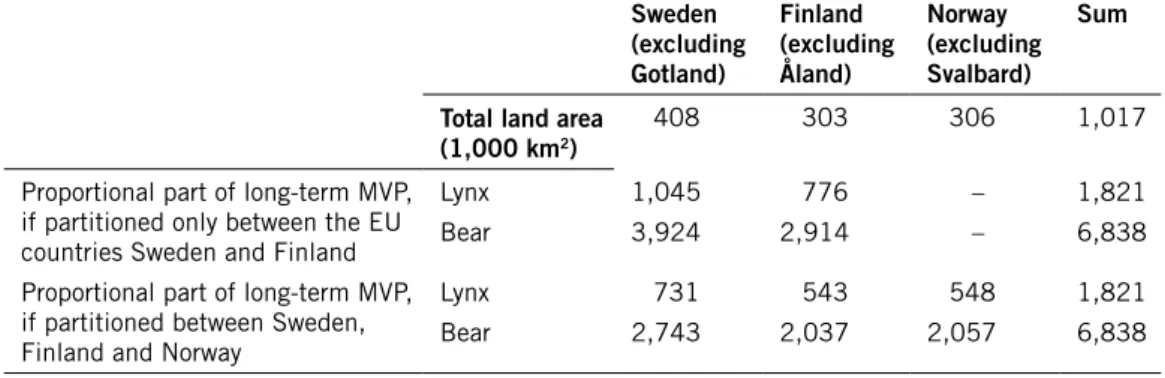
Om en art finns i flera närliggande länder, och om djurens in- och utvandring mellan populationerna i olika länder är tillräckligt omfattande, så behöver inte varje land ha en egen population som motsvarar en långsiktig MVP, utan lång-siktig livskraft kan uppnås genom att en geografiskt och genetiskt samman-hängande population i flera länder sammantaget är tillräckligt stor. Därför har jag också analyserat hur FRP för Sverige skulle kunna sättas genom att fördela arternas långsiktiga MVP, antingen mellan Sverige och Finland, eller mellan Sverige, Finland och Norge.

Några exempel på kortsiktiga kriterier för populationers livskraft är < 10 % utdöenderisk på 100 år och < 5 % förlust av genetisk variation på 100 år. Sådana kortsiktiga MVP-kriterier kan till exempel vara till hjälp om man vill sätta etappmål för en populations utveckling. Jag har uppskattat MVP även utifrån dessa båda kriterier, samt ytterligare tre alternativa kort siktiga MVP-kriterier.

Flera tidigare studier har visat att en måttlig osäkerhet i de ingångsvärden som används i sårbarhetsanalyser, och som beskriver olika aspekter av djurens ekologi och genetik, kan leda till stor osäkerhet i de utdöenderisker som uppskat-tas, och därmed även i de MVP-värden som bedöms motsvara en viss utdöende-risk. En viktig utmaning för naturvårdsbiologer är att göra denna osäkerhet tydlig för beslutsfattare och andra icke-experter som drar slutsatser av sårbarhets-analysernas resultat. Jag har försökt tydliggöra denna osäkerhet genom att ana-lysera flera olika scenarier med varierade värden på ingångsdata för varje art.

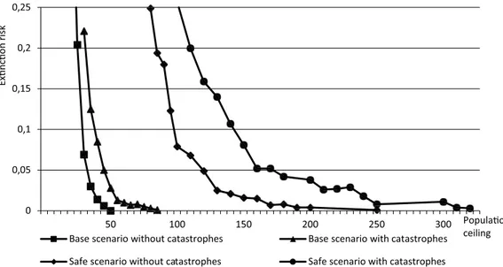
Jag har dels analyserat scenarier som använder de troligaste ingångs-värdena enligt nuvarande kunskap (som jag kallar Base scenarios), och dels scenarier med lite större säkerhetsmariginal i ingångsvärdena (som jag kallar Safe scenarios). Safe scenarios representerar inte värsta tänkbara fall, utan bygger på biologiskt och statistiskt rimliga ingångsvärden fast med en något lägre sannolikhet utifrån de fältdata som finns. Vidare så har både Base sce-narios och Safe scesce-narios analyserats dels med och dels utan inslag av säll-synta katastrofhändelser (till exempel utbrott av nya, allvarliga sjukdomar) som plötsligt dödar mer än halva populationen. Dessutom har björn och lodjur analyserats i olika scenarier baserade på data från två respektive tre olika studieområden i Skandinavien.

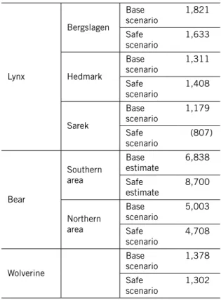
För att komma fram till FRP är de långsiktiga MVP-värdena enligt Base scenarios mest relevanta. Dessa blev strax under 1 400 för järv, mellan 5 000 och 6 900 för björn utifrån data från de två studieområdena, och mellan 1 100 och 1 900 för lodjur utifrån data från de olika studieområdena:

Art data från studieområde långsiktig mvP

Järv 1 378 Björn Södra 6 838 Norra 5 003 Lodjur Bergslagen 1 821 Hedmark 1 311 Sarek 1 179

(9)

Om man tar det högsta av dessa värden för respektive art, fördelar det antalet djur ungefärligen efter ytan av möjligt habitat för arten i Sverige, Finland res-pektive Norge, och sedan avrundar uppåt till närmaste hundratal, så ger det följande förslag på svenska FRP-värden:

Art föreslagen frP

Järv 500

Björn 2 800 Lodjur 800

De kortsiktiga MVP-uppskattningarna varierade kraftigt, både mellan olika MVP-kriterier och mellan olika scenarier. Det kriterium som gav de lägsta MVP-uppskattningarna var kriteriet om < 10 % utdöenderisk på 100 år. MVP-värdena i de olika scenarierna enligt detta kriterium, samt det kortsik-tiga genetiska MVP-kriteriet om < 5 % förlust av genetisk variation på 100 år, framgår av tabellen nedan.

Om man bland dessa MVP-uppskattningar väljer att för varje art fokusera på det högsta troliga (Base scenario) värdet med katastrofer inkluderade, så ger kriteriet om < 10 % utdöenderisk MVP-värden på 35 för björn, 210 för lodjur och 150 för järv. Om man på motsvarande sätt väljer MVP utifrån kri-teriet om < 5 % förlust av genetisk variation så blir MVP-värdena 1 100 för björn, 700 för lodjur och 500 för järv. Art Scenario < 10 % utdöenderisk på 100 år < 5 % förlust av genetisk variation på 100 år Lodjur Bergslagen Base scenario Utan katastrofer 30 500 Med katastrofer 40 500 Safe scenario Utan katastrofer 100 500 Med katastrofer 150 600 Hedmark Base scenario Utan katastrofer 50 280 Med katastrofer 65 320 Safe scenario Utan katastrofer 700 1 000 Med katastrofer 1 500 1 700 Sarek Base scenario Utan katastrofer 140 500 Med katastrofer 210 700 Safe scenario Utan katastrofer (> 2 000) (> 2 000) Med katastrofer (> 2 000) (> 2 000)

(10)

Art Scenario < 10 % utdöenderisk på 100 år < 5 % förlust av genetisk variation på 100 år Björn Södra studie-området Base scenario Utan katastrofer 25 1 000 Med katastrofer 35 1 100 Safe scenario Utan katastrofer 45 1 200 Med katastrofer 65 1 300 Norra studie-området Base scenario Utan katastrofer 25 900 Med katastrofer 30 1 000 Safe scenario Utan katastrofer 40 1 000 Med katastrofer 55 1 000 Järv Base scenario Utan katastrofer 90 370 Med katastrofer 150 500 Safe scenario Utan katastrofer 350 700 Med katastrofer 700 1 300

värden för lodjur, björn respektive järv, enligt de kortsiktiga MVP-kriterierna < 10 % utdöenderisk på 100 år respektive < 5 % förlust av genetisk variation på 100 år, uppskattade under olika scenarier för respektive art. (Ingångsvärdena för lodjur i Sarek Safe-scenarierna visade sig ha egenska-per som gör att dessa värden egentligen inte var meningsfulla för denna typ av beräkningar.)

(11)

Summary

Population viability analyses have been performed concerning populations of bear, lynx and wolverine. The main purpose of these analyses was to form part of the scientific basis for Sweden’s reporting to the European Commission according to the Habitats Directive. Estimates of minimum viable popula-tion size (MVP) under the long-term viability criterion of a genetically effec-tive population size (N_e) exceeding 500 were derived in two different ways: using empirical estimates of rates of loss of genetic variation, when such data were available, and otherwise using computer simulations with the program Vortex. The possibility of setting Favourable Reference Population (FRP) values by partitioning these long-term MVP estimates between neighbouring countries is discussed, and the following tentative FRP values for Sweden are suggested: 800 lynx, 2,800 bears, and 500 wolverines.

Population viability was also analyzed in relation to five different short-term viability criteria. Moderate uncertainty in the input parameters describ-ing the ecology and genetics of a population may lead to very high uncertainty in the estimated extinction risk, and also in the resulting MVP values. A cru-cial challenge for conservation biologists is to make this uncertainty in MVP estimates clear and comprehensible to decision-makers and other non-experts. I developed a series of alternative scenarios for each population, with slightly different input parameters, and estimated separate MVP values for each sce-nario. Under the MVP criterion of < 10 % extinction risk in 100 years, the MVP estimates derived from different scenarios ranged between 25 and 65 for bear, between 90 and 700 for wolverine, and between 30 and 1,500 for lynx. If one chooses to focus on estimates from the most likely scenarios, but with catastrophes included, and then among scenarios representing different geo-graphical areas chooses the highest estimate for each species, those MVP esti-mates were 35 for bear, 210 for lynx and 150 for wolverine, under the < 10 % extinction risk criterion. Compared to the other four short-term viability cri-teria, < 10 % extinction risk in 100 years was the criterion giving the lowest MVP estimates.

In most cases, term genetic MVP values were higher than the short-term extinction risk MVP values; hence, populations meeting the extinction risk criteria will often not fulfill the genetic MVP criteria. Under the short-term genetic MVP criterion of < 5 % loss of genetic variation in 100 years, the MVP estimates derived from different scenarios varied between 900 and 1,300 for bear, between 370 and 1,300 for wolverine, and between 280 and 1,700 for lynx. If one chooses to focus on estimates from the most likely sce-narios, but with catastrophes included, and then among scenarios represent-ing different geographical areas chooses the highest estimate for each species, those MVP estimates were 1,100 for bear, 700 for lynx and 500 for wolver-ine, under the criterion of < 5 % loss of genetic variation in 100 years.

The author alone is responsible for the contents of the report; hence, the views and conclusions presented should not be taken as or referred to as the views or position of the Swedish Environmental Protection Agency.

(12)

Introduction

In 2013, all member states of the European Union are obliged to report the conservation status of species listed in the annexes of the Council Directive 92/43/EEC on the Conservation of Natural Habitats and of Wild Fauna and Flora (briefly: the Habitats Directive). The analyses presented in this report are primarily intended as part of the scientific basis for Sweden’s reporting concerning the bear (Ursus arctos), the lynx (Lynx lynx) and the wolverine

(Gulo gulo).

In May 2012, the Swedish Government commissioned the Swedish Environmental Protection Agency (Naturvårdsverket) to prepare Sweden’s reporting under the Habitats Directive by presenting new population viability analyses for the four large carnivore species occurring in Sweden: wolf (Canis

lupus), bear, lynx and wolverine. An analysis for the wolf has been produced

by Chapron et al. (2012), and I was given the task to produce analyses of the other three species.

The analyses presented here are also intended to form support for further development of the national management plans for the three species. National management plans for bear, lynx and wolverine have been established by Naturvårdsverket in 2012, but these may be complemented with management goals based on population viability analyses.

Favourable Conservation Status and Favourable

Reference Population

In Article 1i of the Habitats Directive, the concept of Favourable Conservation Status (FCS) is defined as follows:

“conservation status of a species means the sum of the influences acting on the species concerned that may affect the long-term distribution and abun-dance of its populations within the territory referred to in Article 2; The conservation status will be taken as ‘favourable’ when:

– population dynamics data on the species concerned indicate that it is maintaining itself on a long-term basis as a viable component of its natural habitats, and

– the natural range of the species is neither being reduced nor is likely to be reduced for the foreseeable future, and

– there is, and will probably continue to be, a sufficiently large habitat to maintain its populations on a long-term basis”

(13)

As pointed out previously, e.g. by Laikre et al. (2009), this definition shows that a) to have FCS, the species needs to be a “viable” component of its habitats;

hence, the legal concept of favourable conservation status has a clear connection to the scientific concept of population viability: a population being viable is a necessary, but not sufficient, requisite for its conservation status to be favourable;

b) to have FCS, the species must maintain itself “on a long-term basis”; hence, short-term viability is not sufficient, but long-term viability is required; c) FCS includes three components, each of which must be favourable for

the conservation status of the species or population to be favourable: not only must the status of the population be favourable (i.e., long-term pop-ulation viability), but also the distribution of the species and the distribu-tion of its habitat must be favourable.

The analyses presented here primarily focus on long-term and short-term population viability. The components of FCS regarding the distributions of the species and their habitats will have to be addressed separately.

In a note from the European Commission (2005), member states are encouraged to base their assessments of species conservation status on refer-ence values for populations and their distributions. The Commission defines Favourable Reference Population (FRP) as

“Population in a given biogeographical region considered the minimum necessary to ensure the long-term viability of the species”

Hence, one requisite for a population to have FCS is that the population meets FRP, and the Commission’s definition of FRP explicitly focuses on long-term population viability.

Population Viability Analysis and Minimum

Viable Population

Population viability analysis (PVA) is a concept that summarizes various types of analyses of a population’s extinction risk, its loss of genetic variation and/ or its degree of inbreeding. If a criterion for population viability has been chosen, then a PVA can be used to estimate what population size is needed to meet that criterion, and this population size is then termed the minimum viable population (MVP). The value of MVP for any population is strongly dependent on which criterion is applied.

Small populations will in the long run lose much of their genetic varia-tion, making them less able to adapt to a changing environment. Within the scientific community of conservation biologists, there is a broad unanimity that to be viable in the long term, a species or population must have what is called a genetically effective population size of 500 or more (e.g., Allendorf &

(14)

Ryman 2002, Laikre et al. 2009, Liberg et al. 2009, Frankham et al. 2010). Genetically effective population size, usually denoted N_e, is principally a measure of how quickly genetic changes take place in a population, e.g. how fast the population loses genetic variation. N_e is affected by the actual size of the population (often denoted N), but also by many other factors such as sex ratio, differences in lifetime reproductive success between individuals, and population fluctuations. In general, N is several times larger than N_e, so an effective population size of 500 may correspond to an actual population of a few thousand animals.

N_e > 500 is the most well-established criterion for long-term population viability. If the ratio N_e/N is estimated for a given population, then the actual population size required to meet the long-term viability criterion N_e > 500 can be calculated from that ratio, and that population size can be termed a long-term MVP for the population.

Some criteria that may be used for short-term population viability assess-ments are < 10 %, < 5 % or < 1 % extinction risk within 100 years, losing < 5 % of the genetic variation within 100 years, and upper confidence limit for loss of genetic variation in 100 years < 5 %. MVP estimates relating to any of these criteria may be termed short-term MVPs.

The extinction risk of a population is determined by the population’s size, its demographic rates (reproduction and mortality), and by various kinds of stochasticity, i.e. random events, including environmental fluctuations between years and inbreeding effects. When MVP estimates are intended as a basis for setting management goals or assessing the conservation status of a population, they should as far as possible take into account all factors that may be import-ant in affecting extinction risk (cf. Akcakaya & Sjögren-Gulve 2000, Ralls et al. 2002, O’Grady et al. 2006, Frankham 2010, IUCN 2011).

In the commission underlying the present study, the Swedish Government explicitly said that MVPs according to the criterion of < 10 % extinction risk within 100 years should be presented. An estimated extinction risk of 10 % or more within 100 years is one of five criteria qualifying a population for being classified to threat category Vulnerable (VU) in the system of threat classifica-tion (e.g., IUCN 2011) developed by the Internaclassifica-tional Union for Conservaclassifica-tion of Nature, IUCN. Linnell et al. (2008) suggested that < 10 % extinction risk in 100 years could be one of several criteria for FRP, and hence for FCS, but that suggestion was not motivated from the definition of FCS in the Habitats Directive, nor from the definition of FRP established by the European Commission (2005). However, as pointed out also by Jamieson & Allendorf (2012), short-term MVPs may be useful in setting short-term management goals.

In the present study, I estimate MVPs both according to the < 10 % extinction risk criterion as requested by the Government, according to four alternative short-term criteria for comparison, and according to the long-term viability criterion of genetically effective population size > 500.

(15)

Dealing with uncertainty and variability

Ludwig (1999) and Ellner et al. (2002) showed that moderate uncertainty about deterministic growth rate (or the factors that determine growth rate) leads to large uncertainty about extinction risk. This lead them to question the usefulness of making quantitative predictions from PVA, and also to ques-tion the relevance of such predicques-tions for management decisions. On the other hand, if quantitative PVA were absent or ignored, important manage-ment decisions would instead have to be based on intuitive expert opinion. Although PVA modelling has its shortcomings, its methods are transparent, and both methods and input data may be subject to continuous improvement, which makes it strongly preferable over such expert assessment (cf. Burgman et al. 2011, Brook et al. 2011).

Realizing both the necessity of using PVA and the considerable uncertainty in its output, a crucial challenge for conservation biologists is to make this uncertainty and its implications clear and comprehensible to decision-makers and other non-experts. This cannot be done merely by providing standard errors or confidence limits for simulation outputs; such figures describe the variation in the output, provided that the mean values of the input param-eters are correct, but they do not reflect the uncertainty caused by the fact that mean values of input parameters may differ from the true mean values of the population. Neither will the application of several different modelling approaches to the same input data achieve this task; parallel use of alternative modelling techniques is wise because it may reveal to what extent the output is dependent on the modelling procedure, but it does not illustrate the effects on PVA output of uncertainties in the estimates of the parameters describing the population. Similarly, sensitivity analysis is useful for describing for which input parameters a slight change of input values will give a relatively large change of output, but often do not combine effects of the known uncertainties of different input parameter values to illustrate how large the uncertainty of the estimated MVP actually is.

The approach used here is to model a series of alternative scenarios for the population of each species, where some scenarios represent what is most likely, given the available knowledge (here termed Base scenarios), while other scenarios make use of alternative – but biologically and statistically reasonable – input values to err on the safe side (here termed Safe scenarios). This is in line with the recommendation of e.g. Reed et al. (2002) to provide a range of predicted values rather than relying on a single point estimate of MVP.

Ideally, I think the result of analysing a Safe scenarios should have a sta-tistically defined probability, e.g. 5 or 10 % probability that reality is that bad or worse. In modelling the Scandinavian wolf population, Nilsson (2004) came rather close to this ideal, by iteratively fitting the input values for extra safety scenarios so that they gave the population a 5 % probability of grow-ing as fast as the population had actually done durgrow-ing a period of 20 years. However, that approach was possible because the population was very small,

(16)

had grown rapidly for an extended time period, and had been closely moni-tored during this population growth. This was an unusual combination of circumstances, and the situation is not comparable for the bear, lynx and wol-verine populations modelled here.

Therefore, in the present study I developed the Safe scenarios in a way that should be more generally applicable than the approach described in the previ-ous paragraph. For input parameters for which there were empirical estimates for the actual populations, I added or subtracted 0.48 times the standard error (SE) to the estimated mean. Adding 0.48 SE to an estimated mortality rate implies that there is 31.6 % probability that the true mortality rate in the pop-ulation is that high or higher. Similarly, subtracting 0.48 SE from an estimated proportion of females producing young implies that there is 31.6 % probabil-ity that the true proportion in the population is that low or lower. If mortalprobabil-ity rates and reproductive rates are measured independently of each other, it is not far-fetched to think that the probability of both these being that unfavour-able or worse should be in the vicinity of (31.6 %)2_{, which is 10 %. Such an}

MVP-value should not be neglected as being extremely unlikely, as may easily be done with a worst-possible-case MVP estimate.

For the effects of inbreeding depression on demographic rates, there are no empirical estimates available for the modelled wild populations, nor for any other free-living populations of the same species. To find out what would be reasonable input values, I gathered values from studies of other mammal populations under natural or semi-natural conditions, and in the Base scenar-ios I used the mean of the values calculated for those other populations. Since uncertainty is much larger when input values are based on data from other species in other environments, I used the mean plus 1 standard deviation (SD) of the values for those populations in the Safe scenarios.

An important factor affecting population viability, for which published studies provide little empirical basis for input data, is the effect of between-year environmental variation on the demographic rates, i.e., the environ-mental stochasticity. In the program Vortex (Lacy et al. 2005), which was used in the present study, environmental stochasticity is modelled by defining standard deviations (SD) for the annual probabilities of females reproduc-ing and of animals dyreproduc-ing. Most published estimates of demographic rates for the three modelled populations are based on pooling data from several years, and the standard errors (SE) presented contain both within-year and between-year-variation. Furthermore, since the number of individuals studied usually varies between years, SE-values for demographic rates based on the whole data set cannot readily be transformed into between-year SD-values, which otherwise might be taken as an upper limit for environmental stochas-ticity. Therefore, as suggested by Miller & Lacy (2005), I partially needed to base the values of environmental stochasticity on biologically reasonable guesses. Since the modelled populations all represent relatively large, long-lived, carnivorous mammals living in a boreal and alpine environment, I chose to use estimates of environmental stochasticity in one of the species as

(17)

the basis for guessing the amount of environmental stochasticity affecting the same demographic rate in the other two species1_.

A separate kind of uncertainty relates to the geographic representativity of the studied segments of the populations. Variation of demographic rates between different parts of a species’ range is not in itself an uncertainty, but it leads to uncertainty about how to draw inferences from data collected in one or a few study areas. For the bear and lynx, which inhabit a larger part of Scandinavia and a wider climatic range, I developed separate Base- and Safe-scenarios for different study areas (two study areas for bear and three for lynx). The differences between these geographic scenarios will illustrate how MVP may vary depending on what the field data look like and in which part of the country the species will occur.

Finally, among the most uncertain aspects in PVA modelling is usually the risk of rare catastrophic events striking the modelled population. In an important review, Young (1994) showed that catastrophic die-offs in wild mammal populations are so widespread in nature that such events must be taken into account in PVAs and in the practical management of endangered populations. To readers in Sweden, the most well-known example of such catastrophic die-offs in wildlife populations is probably the parvo-virus out-break among seals in the late 1980s. A main obstacle to incorporating factors such as the emergence of new, severe diseases in PVA-modelling is that we can never know the absolute probability or frequency of such events. Nilsson (2004) suggested that this problem could be circumvented by defining MVP as a population with a certain chance of persistence, provided that a severe catastrophe occurs. In a similar vein, Chapron et al. (2012) estimated MVP values for wolves both without and with catastrophes of various magnitudes, and presented alternative MVP estimates based on either no catastrophe or inclusion of the most severe catastrophes simulated. Similarly, in this study I run each scenario (Base, Safe, and data from various geographic areas) both without any catastrophe and with a rather severe catastrophe occurring, and present the alternative resulting MVP values.

Partitioning MVPs between countries

If there were little gene flow between the Swedish populations and those of other countries, then the long-term MVPs estimated should be the FRP values for Sweden. However, the populations of all three species seem to be con-tinuous across the Swedish-Norwegian border, and in northern Scandinavia these populations also have more or less contact with Finnish, and indirectly or potentially also with Karelian, populations. Provided that this gene flow is

1 _{An alternative could have been to search the scientific literature for empirical estimates of environmental}

stochasticity for a wide range of different species, and then use estimates based on the mean and range among many other species, but after some initial literature search, I deemed that would be too time-con-suming for this commissioned study.

(18)

sufficient, the FRP for Sweden can be set as a reasonable fraction of the long-term MVP, so to speak representing Sweden’s part of the common responsibility of several countries for maintaining long-term viable populations.

This, however, requires several questions to be answered: When MVPs are used as a basis for FRP / FCS, between which countries can the MVPs then be divided? Should partitioning be proportional to the amount of potential habitat for the species within each country, or should it take into account present-day population sizes or current management goals in the countries? Must the countries agree on this partitioning before any of the states can set an FRP that presumes that other states will take their share of the responsi-bility? So far, neither the European Commission nor the Habitats Committee of the European Union has established any standards or recommendations regarding these issues.

In this report, I demonstrate how the long-term MVPs estimated might be partitioned in a reasonable way, either between the EU member states Sweden and Finland, or between Sweden, Finland and Norway, since Norway too has signed the Bern Convention on the Conservation of European Wildlife and Natural Habitats. Since FCS and FRP are goals aiming at ascertaining long-term viability of the species, my suggestion is that they may be set by partitioning long-term MVPs according to the amount of suitable habitat in the countries, without regarding momentary management goals or popula-tion sizes. Under the assumppopula-tion that partipopula-tioning between all three countries is legitimate, I also propose tentative FRP values for bear, lynx and wolverine in Sweden.

(19)

Material and methods

Population Viability Analysis software

All simulations were performed with the program Vortex version 9.99c (Lacy et al. 2005), which is available at http://www.vortex9.org/vortex.html. The pro-gram is described in detail by Miller & Lacy (2005).

Data collection

Most input data for the simulations were gathered from scientific publica-tions. Jens Persson, Jon Swenson and Henrik Andrén kindly provided advice on what estimate to use for some parameters regarding wolverine, bear and lynx, respectively. Jens Persson also helpfully provided updated figures for litter sizes and litter sex ratio in the wolverine.

Data were not modified to make the simulated populations mimic known population trajectories, due to the limited amount and quality of older moni-toring data.

Study areas

In recent times, ecological field research on lynx has been performed in five study areas in Scandinavia. In the present analysis, I designed scenarios based on data from three of these areas: Bergslagen (around Grimsö, 59° N, 15° E; south-central Sweden, mainly in Örebro county), Hedmark (61° N, 11° E; south-eastern Norway, Hedmark county) and Sarek (around Kvikkjokk, 67° N, 17° E; northern Sweden, Norrbotten county). The study areas are described in more detail e.g. by Andrén et al. (2006) and Nilsen et al. (2012).

Long-term field research on bear is carried out primarily in two study areas in Scandinavia, with marked differences between the reproductive parameters of bears in these areas (Zedrosser et al. 2009), so I designed sepa-rate scenarios also for these. The southern study area was around 61° N, 18° E in south-central Sweden (Dalarna and Gävleborg counties) and south-east-ern Norway, while the northsouth-east-ern study area was around 67° N, 17° E in north-ern Sweden (Norrbotten county). The study areas are described in more detail e.g. by Swenson et al. (2001).

For the scenarios describing wolverine populations, I used pooled data from two study areas: Sarek (around Kvikkjokk, 67° N, 17° E; northern Sweden, Norrbotten county) and Troms (around Dividalen, 68° N, 19° E; northern Norway, Troms county). These study areas are described in more detail by Persson et al. (2006). Inference about the mating system in wol-verines was drawn from genetic data from wolwol-verines in the Sarek area and around the Snøhetta plateau (62° N, 10° E; southern Norway) (Hedmark et al. 2007).

(20)

Input data

initial population

Since the present study primarily aims to support the setting of goals – either long-term or interim goals – for the modelled populations, the estimated MVPs should be based on the extinction risk and heterozygosity loss after a certain population size has been reached. Therefore, in all simulations (except part of the sensitivity analyses) I let the initial population size (N₀) be the same as the ceiling (K) above which the population was not allowed to grow2_{. If}

the simulations instead had been started with a smaller N₀, then the estimated extinction risks would have been elevated by the initial risk of dying out before reaching the population size K. I also let al. simulations start with the stable age distribution calculated by Vortex.

mating system

The program Vortex allows a choice between five types of mating systems, called Monogamous; Long-term monogamy; Polygynous; Long-term poly-gyny; and Hermaphroditic. Among these, neither the monogamous nor the hermaphroditic systems are relevant to any of the three species under study, so the question is whether Polygynous or Long-term polygyny is most accurate. Long-term polygyny implies that a female will reproduce with the same male in successive years as long as the male is alive, while Polygynous means that reproducing pairs are randomly combined in every year of the simulations.

Although males and females live separately for most of the year in all three species, if territories are stable from year to year and males efficiently exclude other males from mating with females within their territory, the mating system may be best represented as Long-term polygyny. For wolverine, the genetically based data in Appendix 1 of Hedmark et al. (2007) reveal no certain case of multi-paternity among 36 litters, and among 10 females known to have pro-duced young in more than one year, only 2 exchanged their partner between years. These results are compatible with a mating system where males effi-ciently monopolize the females within their territory and females take new males primarily when their former partner dies. Hence, I used the option of Long-term polygyny for wolverine.

For bear, on the other hand, Bellemain et al. (2006) found multiple pater-nity in 14.5 % and 28 % of litters with at least 2 and at least 3 cubs, respec-tively. This suggests that dominating males do not monopolize individual females very efficiently, but rather that there is a considerable degree of ran-domness in which male mates with which female in a given year, so I simu-lated the bear populations as being Polygynous without any long term pair bonding.

2 _{This is different from the situation when the aim of a PVA is to assess the actual extinction risk of a}

population at current circumstances. In such cases, the initial population should as much as possible resemble the current population, e.g. with regard to its size and age distribution.

(21)

For lynx, I found no conclusive empirical data to base this choice on. However, considering that females’ home ranges show little overlap and that a male’s home range often encompasses several females (Mattisson et al. 2011), and also that the high proportion of females breeding annually (Nilsen et al. 2012) implies that often several females within the same male territory will be in oestrous simultaneously, I judged it most likely that male monopolization of females is not very efficient in lynx. Hence, also the lynx populations were simulated as being Polygynous with partners randomly combined every year.

demographic rates

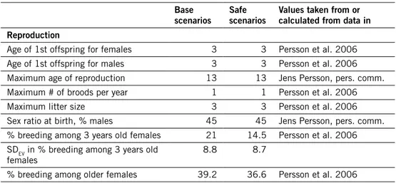
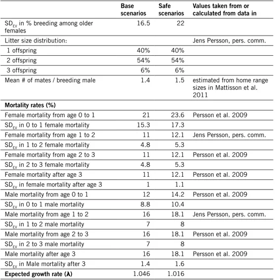
Input values for reproduction and mortality are summarized in Table 1 for wolverine, Table 2 for bear, and Table 3 for lynx. Values for Base scenarios are the most likely estimates according to the empirical studies. Values for Safe scenarios were calculated from the empirical estimates and their standard errors, as described in the Introduction, section “Dealing with uncertainty”.

For lynx and wolverine, values describing the annual proportion of females breeding were taken directly from the literature3_{. For bear, the}

propor-tion of females breeding was calculated from litter intervals, as suggested by Miller & Lacy (2005).

Litter size for wolverines was described as probabilities of having one, two or three cubs in a litter. For bear and lynx, litter size was described by its mean and standard deviation.

The mortality rates I used were those calculated excluding mortality from legal hunting4_{. While poaching is unpredictable and should be included in the}

stochastic process modelled, the amount of legal hunting is exactly known and determined by society, and will probably be ceased at some stage before a population goes extinct. Therefore I judged it preferable to use mortality rates excluding legal hunting mortality. This choice was also related to the aim of the study being to provide a basis for setting goals, rather than to assess the actual extinction risk faced by each population under current circumstances. The mortality rates estimated for subadult wolverines by Persson et al. (2009) were lower than those estimated for adults, but the authors suggested that this may be an artefact caused by a high number of censored individuals in the subadult age class. Jens Persson (pers. comm.) judged it highly unlikely that subadults, most of which have recently left their mother and wandered off to search for a vacant area to settle in, would have lower mortality than the adults. Therefore, I applied the mortality rates estimated for adults also to the subadults.

3 _{The proportion of female wolverines breeding given in Table 1 of Persson et al. (2006) was based on}

counting during the denning season in early spring, while litter size frequencies and juvenile survival were measured among litters still present in May-June. To combine these values without exaggerating the recruitment rate, I reduced the proportion of breeding females to account for that 30 % of the litters found in early spring were lost before the young were counted. Furthermore, using information given in the text of Persson et al. (2006), I estimated different proportions breeding among 3-years-old and older females.

4 _{An exception from this is that the mortality rates used for juvenile wolverines include a small fraction of}

(22)

Given the annual proportion of females breeding and the sex ratio among adults in the population, the annual proportion of males breeding can be esti-mated from the mean number of females esti-mated per successful male, or vice versa. However, both the proportion of males breeding and the number of mates per successful male are rarely known for wild animals. Vortex uses the life table generated from other demographic parameters to estimate the adult sex ratio, and then calculates the number of mates the average successful male must have to achieve the estimated proportion breeding among females, if no males are excluded from the pool of potential breeders. As an alternative, for lynx and wolverine, I calculated the ratios of male to female home range sizes and multiplied this ratio by the proportion of females breeding; this might give a fair approximation for the number of mates per male. For Safe scenarios, I took the ratio of male home range size plus 0.48 times its standard error, divided by female home range size minus 0.48 times its standard error. In cases when this approximation gave a higher number of mates per male than the minimum value suggested by Vortex, then I used the value based on home range sizes and let Vortex calculate the corresponding proportion of males in the breeding pool.

For the bear populations, however, I adopted a different approach. The proportion of males breeding has an effect on the rate of loss of genetic varia-tion, and Tallmon et al. (2004) have provided an empirical estimate of the rate of heterozygosity loss in the southern bear population. Therefore, I ran a series of simulations with demographic parameters for the southern bear population, initial population size and ceiling equaling 700 individuals, and 2,500 simula-tion runs for each tested value of proporsimula-tion of males breeding. In this way, I iteratively found a proportion of males breeding which gave the rate of het-erozygosity loss observed in the real population. Then I used the same propor-tion of males breeding also in the simulapropor-tions of the northern bear populapropor-tion.

Alternatively, I could have used the annual proportions of male bears breeding estimated by Zedrosser et al. (2007). However, within the Scandinavian bear population, most female bears are concentrated in four core areas, while the distribution of male bears is several times larger (Swenson et al. 1998) because many male bears disperse out of the core areas to reside in areas where few mating opportunities are given. Therefore, since two of the female core areas also are the study areas for which proportions of males breeding were estimated by Zedrosser et al. (2007), I suspected those estimates were unrepresentative of the total bear population.

life table analysis

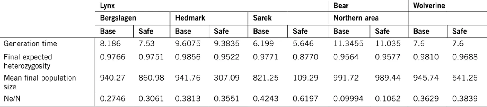
Life tables for both sexes were set up for the Base and Safe scenarios of each species-area combination. The deterministically expected annual growth rate, λ, was calculated from the female life table for each scenario (Tables 1, 2 and 3). Generation time for each scenario (Table 6) was calculated as the mean between the values calculated for each sex.

(23)

For all that is known, the lynx and bear populations have grown well during the second half of the 20th_{century, and the wolverine population has}

deve-loped positively in the last decade. Based on monitoring results, the annual growth rate of the bear population in Sweden 1987–2007 has been estimated at 4.5 %, in spite of hunting, and the number of documented wolverine litters has increased by 3.8 % per year in Sweden and by 5.3 % per year in Norway between 1996 and 2010 (Liljelund 2011). Outside the reindeer husbandry area, the estimated number of lynx family groups (females accompanied by young) in Sweden increased from 111 groups in 1994 to 208 groups in 2000 (Liberg & Andrén 2006), i.e. by 11 % per year. Hence these animals are capa-ble of consideracapa-ble population growth. Considering that there is uncertainty also in the growth rates estimated from monitoring results, the growth rates calculated from the Base scenario parameter values here are compatible with the population growth known to have occurred in the modelled populations. The parameter values used in the Safe scenarios make such population growth less likely, as intended, but not impossible (with one exception, the lynx Sarek Safe scenario).

The life table for lynx based on the demographic data of the Sarek Safe scenario revealed that these demographic rates would give the population a negative deterministic growth rate (λ < 1), which means that if such a demo-graphy were constant over an extended time period, the population would shrink to extinction even without any kind of stochasticity (random events and processes). If that were true, the population could not be considered viable irrespective of its size, and running stochastic simulations of a popula-tion with such a demography is usually considered meaningless. I performed a few analyses on this scenario anyway, for the sake of consistency and for illustrative purposes, but the reader should keep in mind that this scenario is in a sense extreme, although the demographic rates do not differ very strikingly from those of the Sarek Base scenario.

Table 1. demographic input data used in simulations of wolverine populations, and deterministi-cally expected growth rate calculated from life table. how Sd_Ev values were estimated is described in the text (section “Environmental stochasticity”).

Base

scenarios Safe scenarios values taken from or calculated from data in reproduction

Age of 1st offspring for females 3 3 Persson et al. 2006 Age of 1st offspring for males 3 3 Persson et al. 2006 Maximum age of reproduction 13 13 Jens Persson, pers. comm. Maximum # of broods per year 1 1 Persson et al. 2006

Maximum litter size 3 3 Persson et al. 2006

Sex ratio at birth, % males 45 45 Jens Persson, pers. comm. % breeding among 3 years old females 21 14.5 Persson et al. 2006 SD_EV in % breeding among 3 years old

females 8.8 8.7

(24)

Base

scenarios Safe scenarios values taken from or calculated from data in

SD_EV in % breeding among older

females 16.5 22

Litter size distribution: Jens Persson, pers. comm.

1 offspring 40% 40%

2 offspring 54% 54%

3 offspring 6% 6%

Mean # of mates / breeding male 1.4 1.5 estimated from home range sizes in Mattisson et al. 2011

mortality rates (%)

Female mortality from age 0 to 1 21 23.6 Persson et al. 2009 SD_EV in 0 to 1 female mortality 15.3 17.3

Female mortality from age 1 to 2 11 12.1 Jens Persson, pers. comm. SD_EV in 1 to 2 female mortality 4.8 5.3

Female mortality from age 2 to 3 11 12.1 Persson et al. 2009 SD_EV in 2 to 3 female mortality 4.8 5.3

Female mortality after age 3 11 12.1 Persson et al. 2009 SD_EV in female mortality after age 3 1 1.1

Male mortality from age 0 to 1 12 14.2 Persson et al. 2009 SD_EV in 0 to 1 male mortality 8.8 10.4

Male mortality from age 1 to 2 16 18.1 Jens Persson, pers. comm.

SD_EV in 1 to 2 male mortality 7 8

Male mortality from age 2 to 3 16 18.1 Persson et al. 2009

SD_EV in 2 to 3 male mortality 7 8

Male mortality after age 3 16 18.1 Persson et al. 2009 SD_EV in Male mortality after 3 1.4 1.6

Expected growth rate (λ) 1.046 1.016

Table 2. demographic input data used in simulations of bear populations, and deterministically expected growth rate calculated from life table. how Sd_Ev values were estimated is described in the text (section “Environmental stochasticity”); note that for rates > 0.5, the cv_Evvalues used were multiplied by (1 – the rate).

Southern area, Base scenarios Southern area, Safe scenarios northern area, Base scenarios northern area, Safe scenarios

values taken from or calculated from data in

reproduction

Age of 1st offspring for

females 4 4 5 5 Zedrosser et al. 2009, table 1 & 3

Age of 1st offspring for males 3 3 3 3 Zedrosser et al. 2007

Maximum age of reproduction 27 27 27 27 Zedrosser et al. 2007

Max litter size 4 4 4 4 Zedrosser et al. 2009

Mean litter size 2.289 2.289 2.425 2.425 Zedrosser et al. 2009, table 2

SD litter size 0.884 0.884 0.871 0.871 Zedrosser et al. 2009, table 2

Sex ratio at birth, % males 50 50 50 50 Jon Swenson, pers.

comm.

(25)

Southern area, Base scenarios Southern area, Safe scenarios northern area, Base scenarios northern area, Safe scenarios

% adult females breeding 57.5 55.2 41 40 Zedrosser et al. 2009, table 2

SD_EV in # breeding females 17.8 33.1 17.2 24

% of males breeding a certain

year 3.3 3.3 3.3 3.3 iteratively sought to fit the Ne/N ratio meas-ured for the southern population (Tallmon et al. 2004)

Female mortality from age 0

to 1 35 37 4 5.1 Swenson et al. 2001

SD_EV in 0 to 1 female mortality 27.6 29.2 3.2 4 Female mortality from age 1

to 2 17.7 19.3 17.7 19.3 Bischof et al. 2009, table 2

SD_EV in 1 to 2 female mortality 13.5 14.7 13.5 14.7 Female mortality from age 2

to 3 6 6.8 6 6.8 Bischof et al. 2009, table 2

SD_EV in 4 to 5 female mortality 0.54 0.61 0.54 0.61 Female annual mortality after

age 5 6.6 7.2 6.6 7.2 Bischof et al. 2009, table 2

SD_EV in female mortality after

age 5 0.59 0.65 0.59 0.65

Male mortality from age 0 to 1 35 37 4 5.1 Swenson et al. 2001 SD_EV in 0 to 1 male mortality 27.6 29.2 3.2 4

Male mortality from age 1 to 2 8.6 10.2 8.6 10.2 Bischof et al. 2009, table 2

SD_EV in 1 to 2 male mortality 6.5 7.8 6.5 7.8

SD_EV in 4 to 5 male mortality 1.6 1.8 1.6 1.8 Male annual mortality after

age 5 10.7 11.6 10.7 11.6 Bischof et al. 2009, table 2

SD_EV in male mortality after

age 5 0.96 1 0.96 1

Expected growth rate (λ) 1.142 1.123 1.131 1.118

(26)

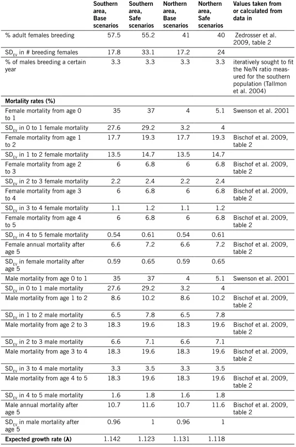
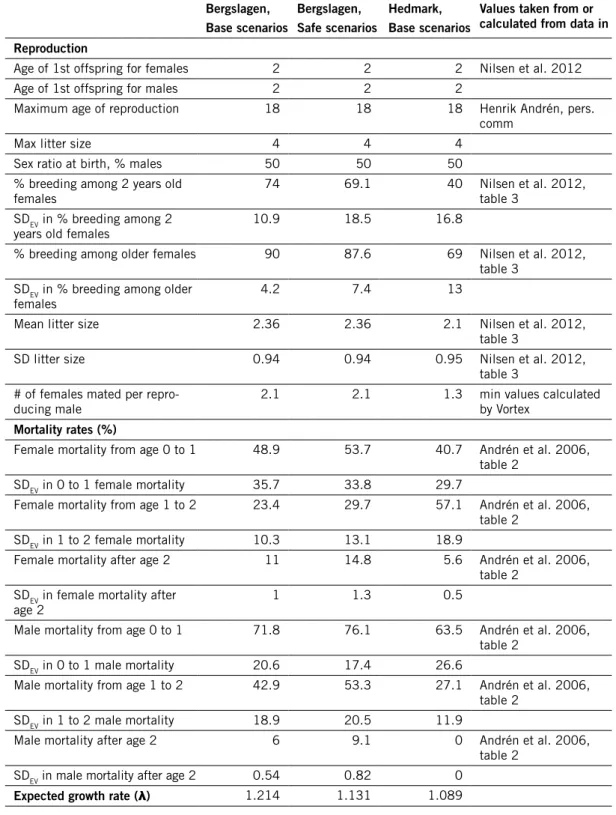
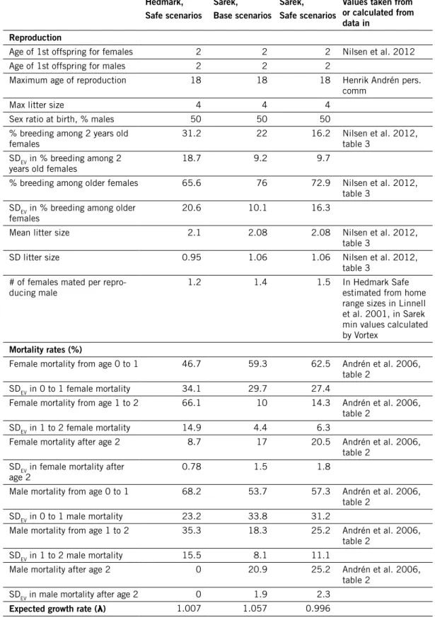
Table 3. demographic input data used in simulations of lynx populations, and deterministically expected growth rate calculated from life table. how Sd_Ev values were estimated is described in the text (section “Environmental stochasticity”); note that for rates > 0.5, the cv_Evvalues used were multiplied by (1 – the rate). (The table continues on next page.)

Bergslagen, Base scenarios Bergslagen, Safe scenarios hedmark, Base scenarios

values taken from or calculated from data in reproduction

Age of 1st offspring for females 2 2 2 Nilsen et al. 2012

Age of 1st offspring for males 2 2 2

Maximum age of reproduction 18 18 18 Henrik Andrén, pers.

comm

Max litter size 4 4 4

Sex ratio at birth, % males 50 50 50

% breeding among 2 years old

females 74 69.1 40 Nilsen et al. 2012, table 3

SD_EV in % breeding among 2

years old females 10.9 18.5 16.8

% breeding among older females 90 87.6 69 Nilsen et al. 2012, table 3

females 4.2 7.4 13

Mean litter size 2.36 2.36 2.1 Nilsen et al. 2012,

table 3

SD litter size 0.94 0.94 0.95 Nilsen et al. 2012,

table 3 # of females mated per

repro-ducing male 2.1 2.1 1.3 min values calculated by Vortex

Female mortality from age 0 to 1 48.9 53.7 40.7 Andrén et al. 2006, table 2

SD_EV in 0 to 1 female mortality 35.7 33.8 29.7

Female mortality after age 2 11 14.8 5.6 Andrén et al. 2006, table 2

SD_EV in female mortality after

age 2 1 1.3 0.5

Male mortality from age 0 to 1 71.8 76.1 63.5 Andrén et al. 2006, table 2

SD_EV in 0 to 1 male mortality 20.6 17.4 26.6

Male mortality after age 2 6 9.1 0 Andrén et al. 2006,

table 2 SD_EV in male mortality after age 2 0.54 0.82 0

(27)

Table 3 continued. hedmark, Safe scenarios Sarek, Base scenarios Sarek, Safe scenarios

reproduction

Age of 1st offspring for females 2 2 2 Nilsen et al. 2012

Age of 1st offspring for males 2 2 2

Maximum age of reproduction 18 18 18 Henrik Andrén pers.

comm

Max litter size 4 4 4

Sex ratio at birth, % males 50 50 50

% breeding among 2 years old

females 31.2 22 16.2 Nilsen et al. 2012, table 3

SD_EV in % breeding among 2

years old females 18.7 9.2 9.7

% breeding among older females 65.6 76 72.9 Nilsen et al. 2012, table 3

females 20.6 10.1 16.3

Mean litter size 2.1 2.08 2.08 Nilsen et al. 2012,

table 3

SD litter size 0.95 1.06 1.06 Nilsen et al. 2012,

table 3 # of females mated per

repro-ducing male 1.2 1.4 1.5 In Hedmark Safe estimated from home

range sizes in Linnell et al. 2001, in Sarek min values calculated by Vortex

Female mortality from age 1 to 2 66.1 10 14.3 Andrén et al. 2006, table 2

Female mortality after age 2 8.7 17 20.5 Andrén et al. 2006,

table 2 SD_EV in female mortality after

age 2 0.78 1.5 1.8

Male mortality after age 2 0 20.9 25.2 Andrén et al. 2006,

table 2 SD_EV in male mortality after age 2 0 1.9 2.3

(28)

Environmental stochasticity

When a series of annual estimates of a demographic rate are available, and also for each year the n-value telling how many animals that year’s estimate was based on, an estimate of environmental stochasticity can be calculated as suggested by Miller & Lacy (2005). The annual n-values are used to estimate the binomial sampling variance for each year and the mean of these (BSV), so that the total between-year variation can be reduced to account for such sam-pling variation. The total between-year variation is measured as the standard deviation SD_tot among the annual rate estimates, and the component of vari-ation caused by environmental fluctuvari-ations is estimated to be SD_EV = square root of (SD_tot2_{– BSV}2_{). In this way, using data on bear cub survival (Swenson}

et al. 2001, table 1) in the southern study area between 1991 and 1998, I estimated mean annual cub mortality rate to 40.9 %, SD_tot to 32 %, SD_EV to 30 % and the environmentally caused coefficient of variation (SD divided by the mean) CV_EV to 73 %. In the years 1987–1990, only 2–5 cubs per year were studied, and in the northern study area only three occurrences of mor-tality were recorded during the whole study period, giving very little basis for analyzing fluctuations in mortality rate. Hence, I applied CV_EV = 73 % to estimate the standard deviation of cub/pup mortality also in the northern bear population, and also in lynx and wolverine.

A data series of annual proportions of females reproducing among wol-verines was presented by Persson et al. (2006, table 1). Following the authors of the paper, I based estimates on the years 1997–2002. However, in this case, the same females were studied over several years and contributed to the annual estimates of subsequent years, suggesting that BSV makes up a larger part of between-year variation than accounted for by the equation SD_EV = square root of (SD_tot2_{– BSV}2_{). Therefore, for the Base scenarios, I instead}

esti-mated environmental stochasticity as SD_EV = (SD_tot– BSV). For wolverine, this gave SD_EV = 24 % and CV_EV = 42 %, so I applied this CV_EV to proportion of females reproducing also in the bear and lynx simulations; for lynx, however, since the proportion reproducing was larger than 50%, I instead multiplied this CV_EV by the proportion not reproducing. For the Safe scenarios, I esti-mated CV_EV from the wolverine data by the same equation as for bear cub mortality (previous paragraph), which gave SD_EV = 35 % and CV_EV = 60 %, and then applied this CV_EV also to the Safe scenarios for bear and lynx, analo-gously to how it was done in the Base scenarios.

Sæther et al. (1998) estimated age-specific bear survival rates and their environmental stochasticity under a model where ϕ and ψ described the expectation and standard deviation, respectively, of annual survival. β = eϕ_/

(1 + eϕ_{) is the survival rate when ψ equals zero. Defining β’ = e}ϕ–ψ_{/ (1 + e}ϕ–ψ₎

and using the β- and ψ-values for the southern study area given by Sæther et al. (1998, table 1), I estimated CV_EV for mortality at different ages as CV_EV = (β’–β) / (1–β). This gave CVEV = 76 % for mortality between age 1 and 2,

CV_EV = 36 % for mortality between age 2 and 3, CV_EV = 18 % for mortal-ity between age 3 and 4, and CV_EV = 9 % for mortality of bears from age 4

(29)

and older. The ψ-values for the northern study area presented by Sæther et al. (1998) suggest lower environmental variation, but are based on fewer occur-rencies of mortality, so I used the CV estimates just mentioned for both popu-lations. For subadult lynx and wolverine, I used CV_EV = 44 %, i.e. the mean of the values calculated for bear between ages 1–4, and for adult lynx and wol-verine mortality I used 9 % as estimated for bear. When a mortality rate was > 50 %, I multiplied the CV_EV by the survival rate instead.

Assuming that environmental variation in reproduction is strongly affected by food abundance, while environmental variation in survival (except for cubs/pups) is mainly determined by other environmental factors, in all simula-tions I let reproduction and mortality vary independently of each other.

inbreeding depression

The strength of inbreeding effects on the demography of a population, i.e, the inbreeding depression, depends on the genetic load, i.e., the amount of del-eterious recessive alleles present in the population. This is quantified in terms of lethal equivalents (LE). There were no empirical estimates of LE in the populations I modelled. In the absence of population-specific data on genetic load, Miller & Lacy (2005) suggest using the value of 3.14 LE, which was the mean value found in a seminal review paper by Ralls et al. (1988) on inbreed-ing depression in captive mammal populations. However, later research has shown that inbreeding depression is strongly dependent on the environment the animals experience, and specifically that inbreeding depression often (though not always) is stronger in free-living populations than in captivity (Jiménez et al. 1994, Crnokrak & Roff 1999, Meagher et al. 2000, Keller & Waller 2002, Armbruster & Reed 2005, O’Grady et al. 2006, Halverson et al. 2006, Mills 2012).

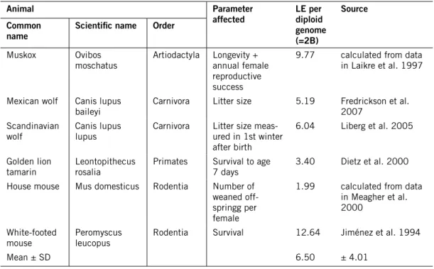
Therefore, I searched for research papers providing empirical estimates of LE in wild mammal populations, or data enabling me to calculate the LE. Most studies reporting inbreeding depression in wild populations infer this from correlations between fitness characters and heterozygosity (not inbreed-ing coefficient)5_{. Such data may be indicative of inbreeding depression, but the}

correlation between heterozygosity and inbreeding coefficient is sometimes low (cf. Pemberton 2004, and references therein), making it questionable to estimate the genetic load in a population without knowledge of inbreeding coefficients. However, I found six studies of different mammal populations where fitness aspects were correlated with inbreeding coefficients so that LE could be calculated (Table 4). When separate estimates of LE were given for males and females, I used those of the females, since in polygynous species it is primarily the females that limit the population growth. The mean value of the six studies then became 6.5, with a standard deviation of 4.01, so

5 _{Also many of the studies quoted in the review papers by Crnokrak & Roff (1999) and Keller & Waller}

(30)

Table 4. Empirical studies providing estimates of lethal equivalents (lE) in wild mammal populations. Animal Parameter

affected lE per diploid genome (=2B)

Source common

name Scientific name Order

Muskox Ovibos

moschatus Artiodactyla Longevity + annual female reproductive success

9.77 calculated from data in Laikre et al. 1997

Mexican wolf Canis lupus

baileyi Carnivora Litter size 5.19 Fredrickson et al. 2007 Scandinavian

wolf Canis lupus lupus Carnivora Litter size meas-ured in 1st winter after birth

6.04 Liberg et al. 2005

Golden lion

tamarin Leontopithecus rosalia Primates Survival to age 7 days 3.40 Dietz et al. 2000 House mouse Mus domesticus Rodentia Number of

weaned off-springg per female

1.99 calculated from data in Meagher et al. 2000

White-footed

mouse Peromyscus leucopus Rodentia Survival 12.64 Jiménez et al. 1994

Mean ± SD 6.50 ± 4.01

I used LE = 6.5 in the Base scenarios and LE = 10.51 (mean + 1 SD) in the Safe scenarios.6

catastrophic events

Among 96 reported instances of catastrophic die-offs among large and middle-sized mammals compiled by Young (1994), he found a relative over-abundance of die-offs reducing the population by 70–90 %, and an under-abundance of die-offs greater than 90 %. In the six reports that concerned large carnivores (African wild dog Lycaon pictus, coyote Canis latrans, and lion Panthera leo), reductions ranged from 50 to 87 %. To simulate catas-trophes within this range of severity, I let survival be reduced by half in one year, and all reproduction failed in that year. The annual probability of such a catastrophe was set at 1 %, so on average there was one catastrophe per simulation run of 100 years.

density dependence

By default, Vortex applies a ceiling model of density dependence, letting all animals exceeding the ‘carrying capacity’ die. To some extent, this is similar to a situation where the human society decides to keep a population below

6 _{An alternative could have been to follow the suggestion of O’Grady et al. (2006) to use a default value}

of 12 LE, which they estimated by comparing twelve studies on different species. However, only three of those studies concerned mammals, while nine were studies on bird populations.