FDI and Economic Growth : An Empirical Study of Lower-middle Income Economies

FDI and Economic Growth

MASTER THESIS WITHIN: Economics

NUMBER OF CREDITS: 30 ECTS

PROGRAMME OF STUDY: Civilekonom

AUTHOR: Qui Ngo

Declaration

This thesis, which is a part of the Civilekonom programme, has been carried out at Jönköping International Business School in the subject area economics. I declare that this thesis is my own work for which I take full responsibility for opinions, findings and conclusions presented. Furthermore, all sources used have been indicated and acknowledged by means of complete references.

___________________________ Qui Ngo

Jönköping International Business School 20th _{May, 2019}

Master Thesis in Economics

Title: FDI and Economic Growth – An empirical study of lower-middle income economies Author: Qui Ngo

Supervisors: Sara Johansson & Pingjing Bo Date: 2019-05-20

Key terms: Foreign direct investment; Economic growth; Lower-middle income economies; Education; Neoclassical growth theory; Endogenous growth theory

Abstract

Within a panel data context with fixed effects method, using data on a sample of 40 lower-middle income economies, this paper investigates whether and to what extent FDI stimulates economic growth over the period 2007-2017. The main finding of this paper highlights the complementary effects between FDI and education, suggesting that a certain level of education must be reached in order for FDI to contribute positively on economic growth. Further, the level of education in this sample set is below the level that is considered as adequate in order to spur economic growth and thus this affects the absorptive capacity. This paper can only confirm that there is a certain association between FDI and economic growth and cannot confirm the widespread belief that FDI stimulates economic growth due to that the estimated models more often than not provided insignificant results.

List of abbreviations

FDI Foreign Direct Investment

FEM Fixed Effects Model

GDP Gross Domestic Product

GNI Gross National Income

M&A Mergers and Acquisitions

OECD Organisation for Economic Cooperation and Development

OLS Ordinary Least Squares

REM Random Effects Model

R&D Research and Development

UNCTAD United Nations Conference on Trade and Development

UNDP United Nations Development Programme

WDI World Development Indicators

Table of Contents

1

Introduction ... 1

2

Background ... 3

3

Theoretical framework ... 6

4

Empirical research ... 11

4.1 The impact of FDI on economic growth ... 11

4.2 The role of absorptive capacity ... 12

4.3 Two-way causality aspect of FDI and economic growth ... 13

5

Data and methodology ... 15

5.1 Data ... 15

5.2 General estimation model ... 15

5.2.1 Variables ... 17

5.3 Econometric analysis ... 18

5.3.1 Unit Root test... 18

5.3.2 Normality test ... 18

5.3.3 Descriptive statistics and correlation matrix ... 18

5.3.4 Estimation method ... 20

6

Empirical findings and analysis ... 21

7

Conclusion ... 26

References ... 28

Figures

Figure 2.1. GDP per capita growth between lower-middle income economies and the world over the

period 1990-2017... 4

Figure 2.2. FDI inflows in economies categorised by GNI level over the period 1990-2017 ... 4

Figure 2.3. FDI inflows and GDP per capita growth in lower-middle income economies over the period 1990-2017 ... 5

Figure 3.1. The role of capital in economic growth theory ... 6

Figure 3.2. FDI theories and their theoretical emphasis... 9

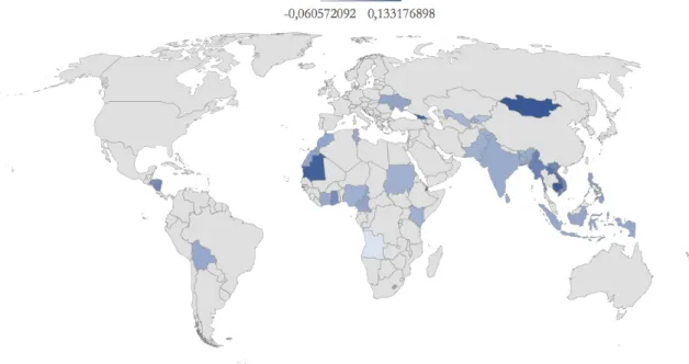
Figure B.1. The distribution of FDI net inflows in lower-middle income economies during 2017... 37

Figure B.2. The distribution of FDI net inflows measured as a percentage share of GDP in lower-middle income economies during 2017 ... 37

Figure C.1. Scatterplots illustrating the relationship between FDI as a percentage share of GDP and economic growth ... 38

Figure E.1. Histogram of normality test ... 40

Figure F.1. FDI inflows as a percentage share of GDP in lower-middle income economies over the period 2007-2017... 41

Figure G.1. Scatterplot of FDI and growth ... 42

Figure G.2. Scatterplot of capital and growth ... 42

Figure G.3. Scatterplot of education and growth ... 42

Figure G.4. Scatterplot of trade openness and growth ... 42

Figure G.5. Scatterplot of corruption and growth ... 42

Tables

Table 5.1. Definition of the variables in the estimation model ... 16

Table 5.2. Descriptive statistics of the variables over the period 2007-2017... 19

Table 5.3. Correlation matrix of the variables over the period 2007-2017... 19

Table 6.1. Estimation results of the determinants of economic growth over the period 2007-2017 .. 21

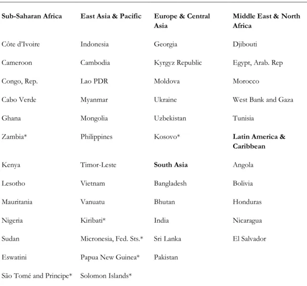
Table A.1. List of lower-midlde income economies ... 36

Table D.1. Test results for unit root on the level of series and in 1st _{difference... 39}

Table E.1. Test results from the Jarque-Bera test ... 40

Table H.1. Test results from the Wald test ... 43

Appendices

Appendix B. The distribution of FDI inflows in lower-middle income economies ... 37

Appendix C. The relationship between FDI as a percentage share of GDP and economic growth .... 38

Appendix D. Unit root test ... 39

Appendix E. Normality test ... 40

Appendix F. Graphical presentation of FDI inflows as a percentage share of GDP... 41

Appendix G. The relationship between economic growth and all the independent variables ... 42

1 Introduction

The role of foreign direct investment (FDI)1 _{in economic growth is a topic that has been}

widely discussed for decades and have resulted in an extensive number of theoretical and empirical works. However, the empirical results are ambiguous and mixed. While some authors state that FDI and economic growth are positively related, others stress that there is no significant relationship. Blonigen and Wang (2004) argue that when using aggregate data that combines both developing and developed countries, it is only the developing countries that show significant evidence for the FDI-growth relationship. Additionally, the factors behind FDI inflows into host countries2 _{are somewhat varied and can differ due to different}

underlying motivations for investment. Despite the mixed results, it is argued that FDI is important for the host country since it generates technology spillovers (OECD, 2002), creates job opportunities (Todaro & Smith, 2011) and provides managerial and organisational skills (de Mello, 1999; Li & Liu, 2005). This implies that FDI spurs economic growth via different channels, mainly from the accumulation of total domestic capital stock and advanced activities within research and development (R&D) through multinational enterprises (MNE). Furthermore, according to de Mello (1999), access to human capital through technology spillovers from MNE’s improves the overall productivity and hence increases economic growth. As a result of the perceived benefits of FDI, policies to attract FDI has been adopted across the world (Hanson, 2001; OECD, 2002). However, there is also a possibility that FDI results in negative crowding out effects. MNEs can easily crowd out domestic firms by having better access to financial resources and hence, gain monopoly power in the market.

UNCTAD (2018) reports that global FDI inflows grew from 23 billion in 1975 to 1.95 trillion by 2017. Lower-middle income economies have also witnessed a significant increase in FDI inflows as well as they have experienced substantial increase in growth rates over the last decades. At the aggregate level, Gross Domestic Product (GDP) for lower-middle income economies grew from 311 billion in 1975 to 6 trillion in 2017 (WDI, 2018). At the same time, FDI inflows accounted for 789 million (0.37% of GDP) in 1975 and 127 billion (1.94% of GDP) in 2017 (WDI, 2019a, 2019b). Furthermore, in 2017, upper-middle income economies received approximately three times more FDI inflow than lower-middle income economies but at the same time, the annual growth rates were similar. This gives rise to the question: Does FDI stimulate economic growth in lower-middle income economies, and to what extent? Hence, the purpose of this paper is to contribute to the ongoing debate about whether FDI stimulates economic growth in lower-middle income economies with data more up to date. A second objective of this paper is to examine the absorptive capacity of the host country and thus, an interaction term between FDI and education as well as an

1 _{If a company has the same production activities in the host market as in the domestic market, this is referred}

to as horizontal FDI. On the contrary, vertical FDI refers to the interest of having different stages of production in different countries.

interaction term between FDI and trade is included in the estimation model. The analysis is based on fixed effects model (FEM) using data on 40 lower-middle income economies following World Bank’s updated classification of GNI level of 20193 _{over the period}

2007-2017 (see Appendix A for a complete list of countries). Additionally, to increase the credibility of the model and avoid omitted variables leading to biased results, other independent variables that may affect economic growth are added into the estimation model. This paper highlights the fact that a certain level of education must be reached in order for FDI to contribute positively on economic growth. Also, the level of education in this sample set is below the level that is considered as adequate to spur economic growth and thus affecting the absorptive capacity. However, this paper can only confirm that there is a certain association between FDI and economic growth and cannot proof empirically the widespread belief that FDI stimulates economic growth due to the fact that the estimation models more often than not provided insignificant results. A possible explanation for the vague results may be due to incomplete specified models that omits other major determinants of economic growth, such as macroeconomic stability, financial development and inflation.

The rest of this paper is structured as follows. Section 2 provides the reader with an overview background of FDI and economic growth, focusing on lower-middle income economies. Section 3 presents a brief review of the theoretical background on the relationship between FDI and economic growth from the perspective of economic growth theories as well as FDI theories. Section 4 provides previous research of related empirical studies. Data collection, general estimation model and method are discussed in Section 5. Empirical findings are presented and discussed in Section 6. Finally, Section 7 summaries the main points and provides suggestions on how this paper can be improved in the future.

3 _{The threshold level for each group is as follows: the classification low income refers to economies with GNI}

per capita of $995 or less; lower-middle income economies $996-$3895; upper middle-income $3896-$12055; high-income $12056 and more (World Bank, 2019).

2 Background

Global FDI inflows accounted for 23 billion (0.49% of GDP) in 1975 and grew to 1.95 trillion (2.35% of GDP) by 2017 (UNCTAD, 2018). Furthermore, UNCTAD (2018) reports that FDI inflows accounts for 39% of the total incoming finance in developing economies. This indicates that the large part of FDI as external source of finance underlies its importance in promoting economic growth in developing countries.

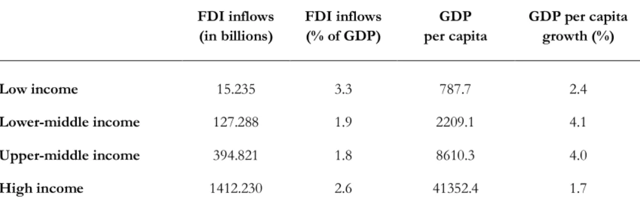
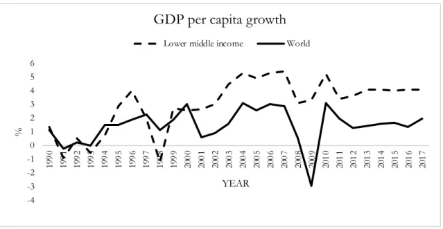
At the aggregate level, GDP for lower-middle income economies grew from 311 billion in 1975 to 6 trillion in 2017 and at the same time, FDI inflows accounted for 789 million (0.37% of GDP) in 1975 and 127 billion (1.94% of GDP) in 2017 (WDI, 2018; WDI, 2019a, 2019b). The attraction of FDI inflows and the increased economic growth rates may have been a result of the work of improving their political and financial institutions during the last two decades which made it possible for the economies to participate in international trade. In 2017, lower-middle income economies experienced similar growth rates as upper-middle income economies and at the same time, the amount of FDI inflows differ quite substantially, as shown in Table 2.1. In fact, lower-middle income economies have experienced higher growth than the total world since 2001, as shown in Figure 2.1. It is therefore interesting to analyse the role of FDI on economic growth, especially in lower-middle income economies. During 2017, India received the highest FDI inflows, a value of 39 billion, followed by Indonesia and Vietnam with 21 billion and 14 billion respectively (see Appendix B for the distribution of FDI inflows in lower-middle income economies). Figure 2.2 illustrates the FDI inflows in economies categorised by GNI level over the period 1990-2017.

Table 2.1. FDI inflows and GDP (2017)

FDI inflows (in billions) FDI inflows (% of GDP) GDP per capita GDP per capita growth (%) Low income 15.235 3.3 787.7 2.4 Lower-middle income 127.288 1.9 2209.1 4.1 Upper-middle income 394.821 1.8 8610.3 4.0 High income 1412.230 2.6 41352.4 1.7

Note: The threshold level for each group is as following: the classification low income refers to economies with GNI per capita of $995 or less; lower-middle income economies $996-$3895; upper middle-income $3896-$12055; high-income $12056 and more.

Figure 2.1. GDP per capita growth between lower-middle income economies and the world over the period 1990-2017

Source: Computed by the author using data from WDI (2019d)

Figure 2.2. FDI inflows in economies categorised by GNI level over the period 1990-2017

Source: Computed by the author using data from WDI (2019a)

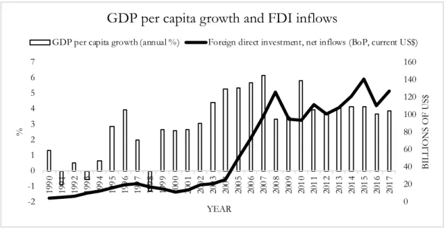
As shown in Figure 2.3, a similar trend can be observed between FDI inflows and GDP per capita growth in lower-middle income economies. As FDI inflows started to increase steadily in the early 2000s, the growth rates for GDP also increased. During the financial crisis in 2008, FDI inflows and GDP growth declined but a quick recovery can be observed, reaching a peak of 140 billion in FDI inflows and 4.12% GDP growth during the year 2015. However,

-4 -3 -2 -1 0 1 2 3 4 5 6 199 0 199 1 199 2 199 3 199 4 199 5 199 6 199 7 199 8 199 9 200 0 200 1 200 2 200 3 200 4 200 5 200 6 200 7 200 8 200 9 201 0 201 1 201 2 201 3 201 4 201 5 201 6 201 7 % YEAR

GDP per capita growth

Lower middle income World

0 500 1000 1500 2000 2500 3000 199 0 199 1 199 2 199 3 199 4 199 5 199 6 199 7 199 8 199 9 200 0 200 1 200 2 200 3 200 4 200 5 200 6 200 7 200 8 200 9 201 0 201 1 201 2 201 3 201 4 201 5 201 6 201 7 B ILLIO NS O F U S$ YEAR

FDI inflows

FDI inflows remain low compared to economies with higher GNI, as can be observed in Figure 2.2. Appendix C presents scatterplots that illustrate the relationship between FDI as a percentage share of GDP and economic growth for each country serving as a sample in this paper.

Figure 2.3. FDI inflows and GDP per capita growth in lower-middle income economies over the period 1990-2017

Source: Computed by the author using data from WDI (2019a, 2019d)

0 20 40 60 80 100 120 140 160 -2 -1 0 1 2 3 4 5 6 7 199 0 199 1 199 2 199 3 199 4 199 5 199 6 199 7 199 8 199 9 200 0 200 1 200 2 200 3 200 4 200 5 200 6 200 7 200 8 200 9 201 0 201 1 201 2 201 3 201 4 201 5 201 6 201 7 BI L L IO N S O F U S$ % YEAR

GDP per capita growth and FDI inflows

3 Theoretical framework

Most empirical studies on the relationship between FDI and economic growth has been based upon neoclassical theory as well as endogenous theory. In contrast to the neoclassical theory that views labour and factor input as determinants of economic growth, endogenous growth theory emphasises the role of human capital and the level of technological innovations. Moreover, whilst the neoclassical model suggests that FDI spurs economic growth via capital stock, the endogenous model suggests that the impact of FDI on economic growth is achieved through the augmentation of the level of knowledge as well as new and better technology (Chenaf-Nichet & Rougier, 2016; de Mello, 1999). Hence, both theories reveal that FDI can spur economic growth as a direct effect as well as an indirect effect.

3.1 Growth theory

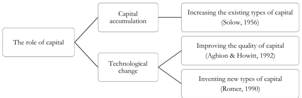
Both theoretical and empirical efforts have identified factors that can affect and/or cause economic growth within an economy based upon growth theory in order to fill the gap between developed and developing countries (De Jager, 2004). Figure 3.1 summaries the main difference on the role of capital on economic growth in the models discussed below.

Figure 3.1. The role of capital in economic growth theory

One of the leading pioneers that provided a mathematically derived growth model back in 1956 was Robert Solow. The Solow growth model breaks the growth of economies into basics where the importance of capital and labour accumulation is being highlighted. An increase in the stock of capital accumulation, which is determined by the savings rate and the rate of capital depreciation only stimulates economic growth in the short-run. According to Barro, Mankiw and Sala-I-Martin (1995), the relationship between capital accumulation and economic growth is positive over time. The model follows the Inada condition4_{, implying}

4 _{The marginal product of capital is very large in a country that has sufficiently low capital stock, and vice versa.}

The role of capital

Capital accumulation

Increasing the existing types of capital (Solow, 1956)

Technological change

Improving the quality of capital (Aghion & Howitt, 1992)

Inventing new types of capital (Romer, 1990)

that developing countries will eventually converge to the same long-run equilibrium capital-to-labour ratio and output per capita as developed countries. The long-run equilibrium is reached when the savings rate equals the required investment. If the savings rate is greater than the required investment, then the capital stock will grow and vice versa. This implies that FDI can help the host country reach a new higher steady state by enhancing the capital stock. Solow (1957) highlights the fact that technological progress is the main driver of long-run economic growth. Nevertheless, no inference to the development of technological progress is provided by Solow, hence the level of technology is assumed to be exogenous. It is believed that labour and capital stock productivity will increase as a result of new technology, and this will further lead to more consistent returns of investment (De Jager, 2004). Due to diminishing returns on the marginal product of capital, the impact of FDI on economic growth is only a short-run effect and leaves long-run growth unchanged. Therefore, additional capital investment is unprofitable when the economy is in equilibrium. The only way for an economy to experience long-run growth under diminishing returns on the marginal product of capital is to discover new technologies through investment in R&D. Despite that the Solow model generally serves as the basis of economic analysis, it is important to shed light into the limitations that comes along due to the fact that the model is grossly simplified. The model excludes environmental considerations such as natural resources and pollution. Further, the model relies on the assumption of a closed economy meaning that the government is totally absent5_.

The seminal work of Romer (1986) and Lucas (1988) attempt to explain technological development rather than treating technological progress exogenously given. Romer (1990) and Aghion and Howitt (1992) stress the importance of technological activities but differ in the essence of how they view innovation. The model of Romer (1990) of endogenous technological change highlights that a large population is not enough to stimulate economic growth, rather the rate of growth is determined by the human capital stock in the country. It is believed that technological development is achieved through a population with greater knowledge, education and training and hence, the endogenous growth theory emphasises the role of accumulation of knowledge. For instance, investment made on education increases the productivity of the labour force (Mankiw, Romer & Weil, 1992) as well as the innovative capacity that results in technological development (Aghion & Howitt, 1992). This implies that if the stock of human capital in a country is below what is considered as sufficient, no economic growth may be observable.

Both the model of Romer (1990) and the Schumpeterian model of Aghion and Howitt (1992) highlight the importance of R&D activities for sustaining long-run economic growth but differ in their assumption on how capital deepening spur economic growth. Whilst Romer (1990) argues that new types of capital triggers economic growth, Aghion and Howitt (1992) state that it is rather quality improvement made on the existing good that spur economic growth. This implies that, in an open economy, FDI inflows make it possible for the host

5 _{See Barro, Mankiw and Sala-I-Martin (1995) for a growth model where the focus is to incorporate an open}

country to acquire the benefits of R&D activities which have been conducted in the foreign country. In this manner, FDI brings along technology spillover externalities that in turn will result in higher productivity as well as new innovation. Within the endogenous growth model, FDI is expected to affect growth positively through (i) capital deepening that in turns results in new input and technologies (Borensztein, De Gregorio & Lee, 1998; Nair-Reichert & Weinhold, 2001), (ii) increase in the existing stock of knowledge through labour training and technology diffusion (de Mello, 1999) and (iii) a reduced market power of the existing firm and hence competition arises (Grossman & Helpman, 1991). Competition among firms result in new and better innovations and these technological progress spur economic growth in the long-run (Grossman & Helpman, 1991, 1994). Furthermore, Romer (1986) argues that economies need to embrace openness, competition and change in order for an economy to grow.

In summary, the key difference between the Solow growth model and the endogenous growth model is the absence of diminishing returns to capital. All in all, the endogenous growth theory includes technology as an endogenous variable and highlights that larger resources put into the R&D sector leads to new discoveries (Grossman & Helpman, 1991, 1994; Romer, 1986, 1990; Romer, 2012) and hence, explains economic growth.

3.2 Definition of FDI

According to the International Monetary Fund (2003, p. 6), FDI is defined as “international investment that reflects the objective of a resident in one economy obtaining a lasting interest in an enterprise resident in another economy”. UNCTAD (2000, 2009) further states that foreign investors are only interested in a host country if they obtain 10% of the voting power and differentiates between greenfield FDI and Mergers and Acquisitions (M&As). The former refers to new investment in physical capital in the host country while the latter involves complete or partial takeover of an existing local firm. de Mello (1999, p. 135) defines FDI as “international inter-firm co-operation that involves significant equity stake and effective management decision power in, or ownership control of, foreign enterprises”. This broad definition incorporates allocation of tangible and intangible assets by a foreign enterprise to a domestic firm, such as (i) flows of capital, (ii) R&D, (iii) management skills and (iv) better technology (Balasubramanyam, Salisu & Sapsford, 1999; de Mello, 1999). Hence, the host countries often characterise FDI as a whole package of resources. Furthermore, Dunning (1993) states that there are four types of investment motivations behind FDI: (i) resource-seeking reasons refers to the advantage of natural resources and/or raw materials, (ii) a firm that have the intention to exploit new markets by engaging in the same production activities will engage in market-seeking FDI, (iii) efficiency-seeking is related to reducing operational costs by for example engaging in FDI in host economies endowed with cheap labour and lastly, (iv) strategic asset-seeking refers to a firm that engage in FDI to acquire intangible assets such as acquisition of local capabilities in the form of R&D, knowledge and human capital.

3.2.1 FDI theories

FDI theories can be separated into two fields, the macroeconomic point of view and microeconomic perspective. Whereas the former is associated with international trade and highlights cross-specific factors, the latter focus on ownership and internalisation benefits and are firm-specific (Denisia, 2010). Furthermore, it is believed that the theory of comparative advantage developed by Ricardo (1871) was the first attempt to explain the concept of FDI. According to this theory, countries should focus on producing goods in which they have comparative advantage in and import goods that utilise the countries’ scarce factor(s) in production. However, since this model is centred on perfect mobility of factors at local level6 _{and two products that are meant to be exported/imported between two}

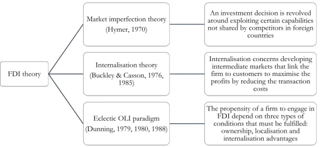
countries, the concept of FDI cannot be explained. Figure 3.2 summarises the selection of FDI theories discussed below.

Figure 3.2. FDI theories and their theoretical emphasis

In his doctoral dissertation from 1960, Hymer explains international production in an imperfect market. He argues that FDI serves as the main function to diversifying the risks of avoiding the structural failures of the market and that market imperfections are created by MNEs. Within this theoretical framework, an investment decision is revolved around exploiting certain capabilities not shared by competitors in foreign countries, such as ownership advantages, product differentiation, low production costs, government incentives and better transportation facilities. Hymer (1970) concludes that FDI only occurs if a firm possess firm-specific advantage that is large enough to reduce the disadvantage of carrying activities abroad since the domestic firms have an advantageous position in terms of culture, language, legal system and even consumer’s preference compared to foreign firms operating abroad. This is also supported by Graham and Krugman (1991). Scholars such as Kindleberger (1969) on the basis of monopolistic power, Knickerbocker (1973) on the basis

6 _{Labour and capital are considered to be mobile domestically but not across borders.}

FDI theory

Market imperfection theory (Hymer, 1970)

An investment decision is revolved around exploiting certain capabilities not shared by competitors in foreign

countries

Internalisation theory (Buckley & Casson, 1976,

1985)

Internalisation concerns developing intermediate markets that link the firm to customers to maximise the profits by reducing the transaction

costs

Eclectic OLI paradigm (Dunning, 1979, 1980, 1988)

The propensity of a firm to engage in FDI depend on three types of conditions that must be fulfilled:

ownership, localisation and internalisation advantages

of oligopolistic power, Buckley and Casson (1976) in the international context as well as Dunning’s (1979, 1988) eclectic paradigm, all support Hymer’s theory. The common thing with these theories is the fundamental belief of the presence of imperfect markets.

Further, Buckley and Casson (1976) conceptualised the internalisation theory and focus on industry-level and firm-level determinants of FDI where they emphasise intermediate inputs and technology. This theory is based on three assumptions: (i) firms maximise profits under an imperfect market, (ii) intermediate products in an imperfect market creates internal markets and (iii) internalisation of markets that take place across the world leads to MNEs. For instance, R&D activities within a firm may develop new technology or inputs that are difficult to export due to high transaction costs. A firm may therefore choose to create their own internal market by backward and forward integration7 _{to keep the transaction cost low.}

Hence, the concept of FDI arises when internalisation involves procedures in different countries.

The eclectic OLI (ownership, localisation and internalisation) paradigm introduced by Dunning (1979, 1980, 1988) is viewed as a major contribution to economic literature since it integrates previous traditional trade and internalisation theories of FDI as well as complement these theories with a new dimension – location. This additional dimension is important since “many of today’s ownership advantages of firms are a reflection of yesterday’s location advantages of countries” (Dunning, 1980, p. 10). He argues that firms only engage in FDI if three conditions are satisfied: (i) it possesses ownership advantages vis-à-vis other firms such as technology, patents, innovation, brand and reputation, (ii) it have certain advantages by locating production activities in a specific area such as business costs, taxes, avoiding trade barriers and low transport costs and (iii) there are some location advantages in using the firm’s ownership advantages in a foreign location. The eclectic OLI paradigm suggests that it does not matter if foreign investors enjoy extensive amount of ownership and internalisation advantages – if its lacks localisation advantages, then domestic investment will be favoured over FDI. Although this theory has been empirically tested by Dunning himself, critics have highlighted the fact that the theory loses operational practicality due to including numerous variables. Also, Boddewyn (1985) claims that changes in only some of the OLI-factors may be enough to explain the successive FDI increases. In summary, all the theories discussed above have different approaches but are united in their view that a firm invests abroad to gain advantages such as location, firm-specific or internalisation of markets.

7 _{The output produced, or the technology developed by one subsidiary may be used as an input in another}

4 Empirical research

Previous research has examined the relationship between FDI and economic growth using both neoclassical and endogenous growth models. The most common research areas studied by scholars have been: (i) the impact of FDI on economic growth, (ii) the role of absorptive capacity in the host countries, and (iii) two-way causality between FDI and economic growth. However, conflicting predictions on the role of FDI on the recipient economy is offered both in theoretical and empirical literature. An overview of these opposing findings provided by previous research discussed below reveals that FDI inflows can either have a positive/negative significant effect on economic growth or even no significance. The size as well as the sign of FDI on economic growth differs due to that different selection of variables, estimation methods, estimation techniques and time periods are chosen by different researchers. Additionally, Nair-Reichert and Weinhold (2001) highlight that the positive impact of FDI on economic growth is the result of positive correlation between them. Hence, cross-country studies may suffer from endogeneity problems and unobserved heterogeneity.

4.1 The impact of FDI on economic growth

Iamsiraroj and Ulubasoglu (2015) highlight that 43% (17%) of the 108 empirical studies examined in their study show a positive (negative) significant effect of FDI on economic growth. Statistically insignificant effects accounts for 40%. The authors also found that within-region variation has a stronger FDI-growth relationship compared to within-country variation. Nunnenkamp (2004, p. 657) argues that “currently prevailing euphoria about FDI rests on weak empirical foundations”. He further states that attracting FDI is an easier task than exerting the benefits from FDI for countries with low per-capita income. Based upon stationary tests on 15 OECD and 17 non-OECD countries over the period 1970-1990, de Mello (1999) finds weak evidence for the impact of FDI on economic growth. He argues that, if FDI enhances economic growth in host countries, then economies whom are referred to as technological leaders are most likely to benefit less from FDI compared to the developing countries. Carkovic and Levine (2002) argues that the positive effects found in previous studies are most likely due to not controlling for endogeneity and the country-specific omitted variables. By employing Arellano-Bond Generalised Moment of Methods, the authors conclude that FDI does not exert an independent influence on economic growth. According to Sarkar (2007), the majority of 51 developing countries over the period 1970-2000 do not support a long-term relationship between FDI and economic growth. This result is irrespective of the level of openness and GDP per capita. For instance, the study of Herzer (2012) reveals that an increase in the FDI-GDP ratio is connected to a long-run GDP decrease (increase) in approximately 60% (40%) of the countries. The main finding from the study conducted by De Gregorio (1992), using panel data of 12 Latin American countries during 1950-1985, is that FDI compared to domestic investment is three to six times more effective. Bende-Nabende, Ford and Slater (2001) conclude that, FDI has positive effects in

ASEAN58_{, both directly and indirectly in Indonesia, Malaysia and the Philippines but}

negative in Singapore and Thailand. The authors also highlight that the host country must have a sufficient level of human capital, adequate infrastructural services as well as having a liberal trade environment in order to benefit from the spillovers produced by FDI indirectly. Vu, Gangnes and Noy (2008) conducted a study on Vietnam and China and found evidence that FDI has statistically significant effect on economic growth both directly and indirectly through labour interactions. Additionally, their findings reveal that the FDI inflows in Vietnam only benefit the manufacturing sector. Pegkas (2015) studied the impact of FDI on economic growth in the Eurozone countries over 2002-2012 and the results indicate a positive relationship. The author used FEM and REM as a part of the method and concludes that a significant factor promoting economic growth in the Eurozone is the stock of FDI. Similar result was found by Campos and Kinoshita (2002). The positive relationship between FDI and economic growth has also been highlighted in more recent studies (Iamsiraroj, 2016; Suliman, Elian & Ali, 2018) where the effects from FDI have shown to be greater in magnitude in developing countries than the developed ones (Makiela & Ouattara, 2018).

4.2 The role of absorptive capacity

In a heterogenous panel data context, Blomstrom, Lipsey and Zejan (1994) find that the benefits, such as technology spillovers, associated with FDI inflows can only be achieved when the host economies reach a certain threshold of development level. Influenced by previous empirical studies, Balasubramanyam et al. (1996) include FDI and exports as additional independent variables (besides capital and labour) and find support for Bhagwati’s (1978) hypothesis – the effectiveness of FDI in fostering economic growth is greater in export promoting countries than countries that apply import substitute strategies. It has also been found that countries with liberalised trade regime tend to benefit most from FDI and hence stimulate economic growth (Bengoa & Sanchez-Robles, 2003; Nair-Reichert & Weinhold, 2001; Zhang, 2001; OECD, 2002). Furthermore, the size of the domestic market is essential as a precondition for attracting FDI (Balasubramanyam et al., 1999) and more importantly, interactions between FDI and human capital spur economic growth (Balasubramanyam et al., 1999; Borensztein et al., 1998; Li & Liu, 2005; Su & Liu, 2016). While domestic investment is important for temporary growth, FDI spurs economic growth in a larger extent than domestic investment (Nair-Reichert & Weinhold, 2001) but only and if only, there exists a minimum threshold of human capital in the host country (Borensztein et al., 1998). Hence, in the process of technological diffusion, FDI and human capital are complementary. Borensztein et al. (1998) further argue that FDI spurs economic growth more if the host country invests in technology progress rather than focusing on increasing the total capital accumulation. For instance, Mansfield and Romeo (1980) argue that FDI is by all means the most inexpensive way of transferring technology. The authors highlight the fact that the transferred technology has already been developed at a high cost in a country with higher resources and hence, the host country can exploit the new technology at a much

lower cost to increase their efficiency in production. Wu and Hsu (2008) did a study covering 62 countries over the period 1975-2000 and found that the impact of FDI on economic growth is positive and significant when host economies have better levels of initial GDP and human capital. However, Djuorvic (2012) highlights that in the past decade, the impact of FDI on economic growth has been positive but the investments made on education is losing their value in the developing countries. According to Dutta, Kar and Saha (2017), countries with lower levels of corruption benefit more from a rise in human capital and vice versa. This implies that a low corruption level in the host country has great importance together with the stock of human capital. Furthermore, low investment is associated with decreasing economic growth. For instance, Mauro (1995) and Mo (2001) argue that a higher perceived corruption in a country lowers both private and public investment substantially. Furthermore, Mo (2001) finds that the level of human capital declines if corruption is observed. On the contrary, some authors state that corruption stimulates FDI (Egger & Winner, 2005) and in turn, FDI spurs economic growth (Okada & Samreth, 2014).

Regarding the study on financial markets, FDI itself shows to have positive effects on economic growth but it is countries with well-developed banking and financial institutions that are able to capture the potential benefits associated with FDI (Alfaro, Chanda, Kalemli-Ozcan & Sayek, 2004; Hermes & Lensink, 2003). For instance, countries that have weak financial systems are all located in Sub-Saharan Africa which attracts a very small share of FDI (Asiedu, 2002) whereas countries located in Latin America and Asia appear to benefit significantly from FDI due to their well-developed financial systems (Hermes & Lensink, 2003). In contrast, Durham (2004) identifies that FDI and economic growth do not have an absolute positive relationship and argues that the effect of FDI on economic growth depends on the absorptive capacity of the host economy. He further argues that FDI inflows are more beneficial in host countries that possess higher institution quality. The study of Olofsdotter (1998) also shows similar findings. Solomon (2011) finds evidence that the level of financial development in the host country and economic growth indicates a non-linear relationship, which contradicts the previous literature. This implies that the FDI-growth hypothesis is independent from the level of financial development.

4.3 Two-way causality aspect of FDI and economic growth

By using a cointegration approach, Granger causality test and Error Correction Model, Zhang (2001) discovered that FDI spurs economic growth in five out of 11 developing countries in Latin America and East Asia, namely Mexico, Hong Kong, Taiwan, Singapore and Indonesia. Chowdhury and Mavrotas (2006) examine the causal relationship using the Toda Yamamoto test for Chile, Malaysia and Thailand. Beside from that the countries are considered as developing countries and major recipients of FDI, their growth patterns and policy regimes differ. Their main findings reveal that FDI does not cause GDP to increase in Chile and in the case of Malaysia and Thailand, bi-directional causality between GDP and FDI was found. In a more recent study, Ahmad, Draz and Yang (2018) found bi-directional relationship between FDI and economic growth in the long-run in ASEAN5 over the period

1981-2013. This indicates that FDI has a more important role in promoting economic growth in East Asia than Latin America. Chakraborty and Basu (2002) found that for the case of India, the causality does not run from FDI to GDP but rather in the opposite direction and that short-run increase of FDI inflows is labour displacing. Additionally, the short-run adjustment process of economic growth in India is not dependent on FDI. Another study on the FDI-growth hypothesis focusing on India, but on a sector level, has been conducted by Chakraborty and Nunnenkamp (2008). By applying a panel cointegration framework over the period 1987-2000, it was found that the importance of FDI was different between the sectors. Whilst no causal relationship in the primary sector was found, the manufacturing sector showed to have a bi-directional causality relation. Within the context of FEM, Hansen and Rand (2006) found evidence on a causal link from FDI to GDP in the short and long-run as well as a long-run impact on economic growth irrespectively of the level of development. As for Scandinavia, whilst Ericsson and Irandoust (2001) found no causal link between FDI and economic growth in Denmark and Finland, in the Granger sense, bi-directional (uni-directional) causality was found in Sweden (Norway). Anwar and Nguyen (2010) argue that a two-way linkage between FDI and economic growth exists in Vietnam, but only in four out of seven regions. The main findings of the authors are that investment made on: (i) education and training, (ii) developing financial marketing, and (iii) diminishing the existing technology gap between the local firms and foreign firms located in Vietnam, enhance the impact of FDI on economic growth. Umoh, Jacob and Chuku (2012) use both single and simulations equation systems in their study where they investigate whether any endogenous effects of FDI on economic growth in Nigeria over the period 1970-2008 can be found. Their findings reveal that FDI not only stimulates economic growth but that the relation is the opposite as well, i.e. bi-directional causality. Caesar, Haibo, Udimal and Osei-Agyemang (2018) find similar findings for China. However, Mah (2010) highlights that FDI inflows have not promoted economic growth, rather economic growth has caused FDI inflows into China. Iqbal, Shaikh and Shar (2010) investigate the causality relationship between FDI, international trade and economic growth over the period 1998-2009 in Pakistan. Their main findings are that the impact of FDI is positive on the trade growth and that FDI inflows into the country was due to Pakistan’s great performance in economic growth during the 21st _{century. Kheng, Sun and Anwar (2017) find significant bi-directional}

causality between FDI and human capital and highlight that higher levels of human capital in a country would most likely attract FDI inflows compared to a country with less human capital.

5 Data and methodology

5.1 Data

The research question whether FDI stimulates economic growth in lower-middle income economies is estimated by short balanced panel data regression9 _{over the period 2007-2017.}

As more recent data for 2018 was missing for many variables of interest, 2017 was chosen as the ending year. Compared to time-series and cross-sectional data, the probability of rejecting a false null hypothesis increases by using panel data since the sample size is greater (Observations = N ´ T). Furthermore, panel data controls for the individual heterogeneity which gives more informative, less collinearity among the variables and more degrees of freedom (Baltagi, 2005; Gujarati & Porter, 2009). The World Bank’s World Development Indicators (WDI, 2019) has been the main source for the specified period for the variables: growth, FDI, capital and trade openness. Average years of schooling has been retrieved from United Nations Development Programme (UNDP). Data on the corruption level is provided by World Governance Indicators (WGI).

5.2 General estimation model

To investigate the relationship between FDI and economic growth in lower-middle income economies over the period 2007-2017, economic growth is modelled as a function of FDI along with other variables that are considered to have great relevance on economic growth by several scholars. Since the variables that should be included in the growth equation are not given from theory, the control variables are motivated by the related existing empirical studies and data availability. Other factors that are considered to have an impact on economic growth are captured in the error term. To examine if FDI has a bigger impact on economic growth in countries with higher education level, an interaction term between FDI and education is included. An interaction term between FDI and trade openness is also included in the estimation model to capture the impact of the combined effect on economic growth. In particular, the estimation model relies on the following equation:

LN Growth*+= a + β/FDI*++ β3Capital*++ β9Education*++ β?Trade*++ βBCorruption*+

+ βCFDI*+ × Education*++ βEFDI*+ × Trade*++ e_*+

(5.1)

where i is the country subscript, t is the time subscript, the sign significance of parameter β

specify how a one-unit change in an independent variable influence change in economic growth and e is the random disturbance term. Since FDI serves as an independent variable and economic growth is the dependent variable, the hypothesis is that FDI in some way affects economic growth. However, one cannot avoid the potential of endogeneity10_{, which}

9 _{The number of cross-sectional (N=40) is greater than the number of time periods (T=10).}

implies that it may be in the opposite direction, namely that higher economic growth attracts FDI to some certain degree. It is difficult to examine how the relationship is in the real world and hence this paper chooses to ignore the latter relationship and only focus on the former. Boreinzstein et al. (1998) and Makki and Somwaru (2004) suggest that a proper instrument to eliminate the problem of endogeneity is to include lagged FDI. A summary of the variables is presented in Table 5.1 whereas the next subsection describes the variables more in depth.

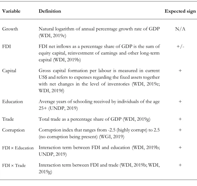
Table 5.1. Definition of the variables in the estimation model

Variable Definition Expected sign

Growth Natural logarithm of annual percentage growth rate of GDP (WDI, 2019c)

N/A

FDI FDI net inflows as a percentage share of GDP is the sum of equity capital, reinvestment of earnings and other long-term capital (WDI, 2019b)

+/-

Capital Gross capital formation per labour is measured in current US$ and refers to expenses regarding the fixed assets together with net changes in the level of inventories (WDI, 2019e; WDI, 2019f)

+

Education Average years of schooling received by individuals of the age 25+ (UNDP, 2019)

+

Trade Total trade as a percentage share of GDP (WDI, 2019g) + Corruption Corruption index that ranges from -2.5 (highly corrupt) to 2.5

(no corruption being present) (WGI, 2019)

+

FDI ´ Education Interaction term between FDI and education (WDI, 2019b;

UNDP, 2019)

+

FDI ´ Trade Interaction term between FDI and trade (WDI, 2019b; WDI,

2019g)

+

The econometric model follows a log-linear model which implies that for relatively small values between -0.1 and 0.1 of the estimation coefficients, the following approximation can be used for a quick interpretation: the expected percentage point change in economic growth for one-unit change in any independent variable is determined by β × 100% on average. However, using the log point change as the approximation results in biased downward estimates of the correct percentage change in economic growth when the estimated coefficient takes on a higher value than 0.1. Hence, the correct approximation is as follows:

a one-unit change in any independent variable result in a percentage change in economic growth by [exp(β) − 1] (Gujarati & Porter, 2009).

5.2.1 Variables

Growth. The dependent variable represents economic growth and is measured as the annual percentage growth of GDP. It has been calculated by taking the natural logarithm of current GDP in US$ and then transformed into percentage growth: MNOP Q MNOPRS

MNO_PRS . This measurement

is standard in the literature since it characterises the change in a country’s development and productivity. A higher GDP growth is associated with a higher level of development in the host country. Hence, GDP growth serves a good proxy for economic growth.

FDI. The data of FDI net inflows as a percentage share of GDP is in current US$ and is the sum of equity capital, reinvestment of earnings and other long-term capital. To circumvent the simultaneity bias associated with the fact that FDI itself is a component of GDP through the national income-accounting identity, this paper uses GDP ratio. Since the FDI-Growth literature is ambiguous, FDI is expected to have either a positive or negative sign. Capital. Gross capital formation is measured in current US$ and refers to expenses regarding the fixed assets together with net changes in the level of inventories. This paper uses capital-labour-ratio to measure the level of capital concentration to prevent biased results – countries with higher labour force would otherwise have a higher value of capital automatically. Education. Average years of schooling received by individuals of the age 25+ to capture investment in human capital is used in this paper. Investment made on human capital spurs innovation by enhancing the productivity of physical capital and labour (Barro et al., 1995; Lucas, 1988; Mankiw et al., 1992; Romer, 1980). Hence, it is expected that a greater level of human capital contributes to a higher productivity, which in turn could increase FDI inflows. Trade. The standard definition of trade openness that has been used widely in scientific papers

is TUVWX+Y Z *[VWX+Y_MNO × 100. More precisely, trade openness consists of the sum of exported and

imported goods and services measured as a percentage share of GDP. The performance of economic growth is most likely to improve if economies focus on specialising goods and/or services in which they have comparative advantage and then export the goods and/or services (Grossman & Helpman, 1994). Moreover, foreign investors may fully exploit economies of scale and scope if the host country employ liberalised trade regimes (Noorbakhsh, Paloni & Youssef, 2001).

Corruption. The corruption index, control of corruption (CC), provided by the WGI serves as a proxy for the corruption level in each country which ranges from -2.5 (highly corrupt) to 2.5 (no corruption being present). Corruption has been argued to reduce the growth rate of a country (Ahmad, Ullah, Arfeen, 2012; Hall & Jones, 1999; Mo, 2001). It is therefore expected that corruption has a negative effect on economic growth.

5.3 Econometric analysis

5.3.1 Unit Root test

An important aspect for any econometric analysis is whether the data is stationary. If the mean and variance are constant throughout the series, then the variable is considered to be stationary. If that is not the case, the variable is non-stationary which would yield spurious regressions and hence, improper for forecasting. Three possible outcomes from a stationary test are: (i) the variables are integrated of order 0 I(0), (ii) the variables are integrated of order 1 I(1) or (iii) a combination of both I(0) and I(1). I(0) implies that the variable is stationary in level and requires no differencing while I(1) implies that the variable is stationary after first differencing.

To check the stationarity of the variables of interest in this paper, Levin, Lin and Chu test (2002) was performed. From the test results (see Appendix D), it is shown that all variables are of I(0). The test rejects the null hypothesis of unit root at 1% significance level for all variables.

5.3.2 Normality test

To determine whether the residuals are normally distributed, the Jarque-Bera test was performed. Under the null hypothesis of the Jarque-Bera test, the test assumes that the data is normally distributed under two statistical properties: (i) the data is symmetric around its mean which indicates a value of zero and (ii) kurtosis takes on a value of three. The Jarque-Bera statistic takes on a quite high value of 60 and the p-value equals 0.0000 and hence, the null hypothesis is rejected at 5% significance level (see Appendix E). This implies that the estimation model as specified in Equation (5.1) may carry misleading information regarding the dependent variable, in this case, economic growth.

5.3.3 Descriptive statistics and correlation matrix

Descriptive statistics for the data in terms of mean, median, maximum, minimum and standard deviation of the variables integrated in the growth equation are presented in Table 5.2. Over the period 2007-2017, the mean value for economic growth was 0.8% whereas the maximum (minimum) value was 7% (-6%). The highest growth rate was experienced by Myanmar during 2008. During 2015, Congo received the highest FDI inflows measured as a percentage share of GDP, yet it experienced the lowest growth rate the same year. A graphical presentation of FDI inflows of the sample set of countries is presented in Appendix F.

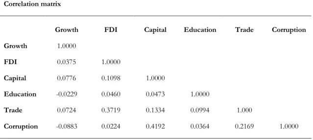
Table 5.3 shows the relationship between the variables in the model and was computed to ascertain whether multicollinearity is presence. Correlation ranges from -1 (perfect negative correlation) to +1 (perfect positive correlation). As shown in the table, FDI, capital and trade have a positive relationship with economic growth. However, the relationship between

education and growth is negative, which contradicts what theory predicts. The table also shows that a higher level of corruption affects economic growth negatively. None of the coefficients takes on high values and hence, multicollinearity is not a problem. Figures G.1-G.5 in Appendix G illustrates the relationship between economic growth and FDI, capital, education, trade and corruption respectively.

Table 5.2. Descriptive statistics of the variables over the period 2007-2017

Descriptive statistics

Variable N Mean Median Maximum Minimum Std. Dev

Growth 440 0.0081 0.0083 0.0748 -0.0665 0.0166 FDI 440 0.0442 0.0277 0.5001 -0.3715 0.0579 Capital 440 1.5207 1.3144 8.9053 0.1685 0.9739 Education 440 6.6682 6.1000 12.8000 2.3000 2.4836 Trade 440 0.0085 0.0087 0.0200 1.67E-05 0.0036 Corruption 440 -0.6023 -0.6577 1.5683 -1.6728 0.5692

Notes: FDI inflows are presented on net basis and hence, a negative sign indicates that at least one of the components that refers as FDI is negative and do not balance by positive amount of the remaining components.

Table 5.3. Correlation matrix of the variables over the period 2007-2017

Correlation matrix

Growth FDI Capital Education Trade Corruption

Growth 1.0000 FDI 0.0375 1.0000 Capital 0.0776 0.1098 1.0000 Education -0.0229 0.0460 0.0473 1.0000 Trade 0.0724 0.3719 0.1334 0.0994 1.000 Corruption -0.0883 0.0224 0.4192 0.0364 0.2169 1.0000

5.3.4 Estimation method

Equation (5.1) is adjusted and tested following the conventional procedure for panel data to examine whether pooled ordinary least squares (OLS), fixed effects model (FEM) or random effects model (REM) would be the appropriate estimation method. A pooled OLS neglect the dual nature of time series and cross-sectional data and assumes that there is no heterogeneity. Under the assumption that the entities behave in the same way, where there is homoscedasticity and no autocorrelation, a pooled OLS would be preferable. Omitted variables that differ across countries but are constant over time are controlled for in FEM, which is equivalent to using dummy variables for each cross-section, also known as Least Squares Dummy Variables (LSDV). Unlike FEM, the error term is uncorrelated with the independent variables and are assumed to be random in REM.

The likelihood ratio test for redundant fixed effects show that χ3 _{= 108.7383 and F-statistic}

= 2.8250. This test suggests that the FEM is adequate because the null hypothesis of fixed effects is redundant is rejected at the 1% significance level for both the χ3 _{distribution and}

F-statistic. In addition, the null hypothesis of the Hausman test (1976) Cov(α*, x*+) = 0 is

rejected (χ3_{= 73.0414 with a p-value of 0.0000). Under the null hypothesis of the Hausman}

test (1976), REM is consistent and appropriate whereas FEM is consistent but inappropriate. Under the alternative hypothesis Cov(α*, x*+) ≠ 0, REM is inconsistent while FEM is

consistent and appropriate. This implies that FEM is more appropriate, leading to more efficient results than REM. Furthermore, the Wald test confirms that the variable FDI is not endogenous since the p-value of the test statistic is greater than 0.05, meaning that FEM is an appropriate estimation method (see Appendix H). The empirical model is thus estimated by FEM and is specified as follows:

LN Growth*+= a + β/FDI*++ β3Capital*++ β9Education*++ β?Trade*++ βBCorruption*+

+ βCFDI*+ × Education*++ βEFDI*+ × Trade*+ + µ*+ e_*+

(5.2)

where i, t and β has the same interpretations as in Equation (5.1). The disturbance term µ*

captures all of the variables that affect LN Growth*+cross-sectionally but do not vary over time.

For instance, the geographical location is very country-specific, meaning that the location does not change over time. Hence, by allowing for different intercepts for each cross-sectional unit, the heterogeneity in µ* can be captured. Furthermore, White’s cross-section

standard errors and covariance is applied to minimise the influence of heteroscedasticity in the error terms.

6 Empirical findings and analysis

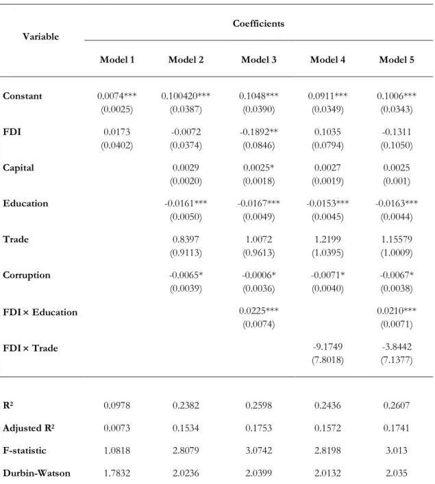
Table 6.1. Estimation results of the determinants of economic growth over the period 2007-2017

Fixed effects model

Variable

Coefficients

Model 1 Model 2 Model 3 Model 4 Model 5

Constant 0.0074*** (0.0025) 0.100420*** (0.0387) 0.1048*** (0.0390) 0.0911*** (0.0349) 0.1006*** (0.0343) FDI 0.0173 (0.0402) -0.0072 (0.0374) -0.1892** (0.0846) 0.1035 (0.0794) -0.1311 (0.1050) Capital 0.0029 (0.0020) 0.0025* (0.0018) 0.0027 (0.0019) 0.0025 (0.001) Education -0.0161*** (0.0050) -0.0167*** (0.0049) -0.0153*** (0.0045) -0.0163*** (0.0044) Trade 0.8397 (0.9113) 1.0072 (0.9613) 1.2199 (1.0395) 1.15579 (1.0009) Corruption -0.0065* (0.0039) -0.0006* (0.0036) -0.0071* (0.0040) -0.0067* (0.0038) FDI ´ Education 0.0225*** (0.0074) 0.0210*** (0.0071) FDI ´ Trade -9.1749 (7.8018) -3.8442 (7.1377) R2 _{0.0978 0.2382 0.2598 0.2436 0.2607} Adjusted R2 _{0.0073 0.1534 0.1753 0.1572 0.1741} F-statistic 1.0818 2.8079 3.0742 2.8198 3.013 Durbin-Watson 1.7832 2.0236 2.0399 2.0132 2.035

Notes: Standard errors in parenthesis are estimated using White cross-section standard errors and covariance. ***, **, * indicate the significance level at 1%, 5%, and 10% respectively. Obs. = 440.

The purpose of this paper is to investigate if FDI stimulates economic growth in lower-middle income economies over the period 2007-2017. A second objective is to examine

whether FDI interacts with human capital and trade to affect the growth rate of the economies in the sample set. Hence, interaction terms are included in the estimation model stepwise. Prior to running the regressions, unit root tests showed desirable patterns for all variables. The main results of the applied panel data estimations regarding the effects of selected determinants on economic growth in middle-lower income economies are presented in Table 6.1. The Durbin-Watson statistic is rather close to two in all the estimated models, meaning that most likely there are no problems with autocorrelation. Thus, HAC Newey-West estimators are not necessary to apply. Additionally, as shown in Table 6.1, the Durbin-Watson statistic takes on a higher value than R2 _{and adjusted R}2_{, implying that the estimated}

models do not suffer from spurious regressions. Given the cross-sectional nature of the sample set, it is reasonable that all the estimation models have generally low R2 _{values. Model}

1 includes FDI as the only independent variable and disregards the control variables. Model 2 includes FDI, capital, education, trade and corruption whereas Model 3 and 4 builds on Model 2 and adds an interaction term between FDI and education and FDI and trade respectively. Finally, the result based on the econometric model specified in Equation (5.2) is presented by Model 5.

Capital is considered to be the main source of economic growth (Solow, 1956, 1957) and this is also true for all the estimated models. Even though capital is only statistically significant at 10% level in Model 3, the standard errors show that capital is not far from being significant in all other models. Since machinery and equipment comes along with FDI, one could argue that FDI is a component in the variable capital itself. It is therefore interestingly that one-unit change in capital increases economic growth by 0.25% whereas one-one-unit change in FDI decreases economic growth by 18%, ceteris paribus. This means that other components in the variable capital must outweigh the negative effect of FDI, making capital positively related to long-run economic growth.

There is unquestionably abundant awareness and theoretical support that human capital is considered as fundamental factor for social and economic development (Barro, 1991; Romer, 1990) since new technology and production process can be adapted and improved much faster when the labour force has a high level of human capital (Borensztein et al., 2008). However, the coefficient for education is negative and significant at 1% significance level for all the estimated models when using mean years of schooling as proxy. This means that the education level measured as the average years of schooling does not deliver on its promise as the key component of economic growth. The coefficients range from -0.0153 to -0.0167 which implies that an additional year of schooling decelerates economic growth by approximately 1.53%-1.67%. Under this proxy, students are assumed to receive the same benefits from a year of schooling and learning. One can argue that this is not necessarily true since different school systems are practiced around the world, meaning that one year of schooling in a lower-middle income economy might not generate the same cognitive skills to the same extent as one year of schooling in a high-income economy. Furthermore, learning that takes place outside the classroom is not accounted for. Hanushek, Jamison, Jamison and Woessman (2008) argue that economic growth accelerates only if higher mean years of schooling result in improvements in cognitive skills. The mean year for school attainment equals six years in this sample, whereas only seven out of 40 lower-middle income economies

have a mean year of school attainment that is equal or greater than 10 years11_{. If the}

population in one country has completed six or even 12 years of schooling on average does not automatically mean that the students enrolled have increased their cognitive skills, which is necessary for economic growth. This implies that the amount of years that students receive education is not the key to economic growth, rather how much students learn while they are in school as well as the education quality. One could also argue that the education level in this sample set is below the level that is considered as necessary to spur economic growth because six years of schooling indicates that education has only been completed at primary level. Some countries such as Bhutan has a mean year of schooling of 2-3 years whereas Côte d’Ivoire, Cambodia, Sudan and Djibouti have a mean year of schooling of 3-4 years. Hence, the investments made on education in the sample set of countries may cost more to the society than what it contributes. This is in line with the finding of Djurovic (2012) that investment made on education is losing its value in the developing countries. Differences in learning achievements could also be an explanation why the results show that education has a negative impact on economic growth.

The coefficients for trade openness are positive in all the estimated models, as expected, but it is statistically insignificant. This implies that trade openness has no influence on economic growth in all countries in the sample set. Bengoa and Sanchez-Robles (2003) and Nair-Reichert and Weinhold (2001) among others argue that countries with liberalised trade regime tend to benefit most from FDI and in turn, FDI stimulates economic growth. However, the results obtained from the regressions cannot confirm such relationship. Since higher values of the CC index indicates less corruption, a positive and significant coefficient would suggest that the relationship between corruption and economic growth is negatively related. The coefficient is statistically significant at 10% level and range from -0.0006 to -0.0071 which implies that when the CC increases, i.e. a decrease in perceived corruption, on average, economic growth will decrease by approximately 0.06-0.71%, ceteris paribus. While the results contradict the findings of Hall and Jones (1999), Mo (2001) and Ahmad et al. (2012), the estimated relationship between corruption and economic growth is more in line with Egger and Winner (2005) and Okada and Samreth (2014). Indeed, the majority of the lower-middle income economies in this paper possess high levels of corruption and has attracted massive amounts of FDI inflows over the years. This result is quite surprising since it has been found that corruption reduces investment in all aspects (Mauro, 1995) which in turn affects economic growth negatively. It is however found that, as illustrated in Figure 2.1, lower-middle income economies have experienced higher growth rates compared to the total world, which supports the conditional converge theory of Solow (1956). This is also true for the study period 2007-2017 in this paper. From the viewpoint of the eclectic OLI paradigm, paying bribes to speed up bureaucratic processes could be seen as a localisation advantage. Hence, foreign investors may want to locate its businesses in countries with higher levels of corruption. If the revenue exceeds the costs for foreign investors, corruption is expected to increase the level of FDI inflow. This is however not