THESIS
ANALYSIS OF ROOT GROWTH IN TWO TURFGRASS SPECIES
WITH MINIRHIZOTRON AND SOIL CORING METHODS
Submitted by Jason Scott Young
Department of Horticulture and Landscape Architecture
In partial fulfillment of the requirements For the Degree of Master of Science
Colorado State University Fort Collins, Colorado
Fall 2015
Master’s Committee:
Advisor: Yaling Qian Co-Advisor: Louise Comas Troy Ocheltree
Copyright by Jason Scott Young 2015
ii ABSTRACT
ANALYSIS OF ROOT GROWTH IN TWO TURFGRASS SPECIES WITH MINIRHIZOTRON AND THE SOIL CORING METHOD
In this study root growth of a turf-type variety of inland saltgrass (Distichlis spicata L. Greene) (a native grass with varieties in development by Colorado State University) and Kentucky bluegrass (Poa pratensis L.) (a common turfgrass planted in the arid and semi-arid west) was examined under saline conditions in a pot experiment and non-saline conditions in the field. Since turfgrass is a high user of water, the turf industry is interested in using native species that use less water and also salt-tolerant species, which may allow the industry to use marginal water (grey water) for irrigation. However, plants with different root distributions will need to have irrigation managed differently. These experiments examined root growth differences in saltgrass and Kentucky bluegrass to begin exploring how these species might need to be managed differently in saline and non-saline conditions. Two separate experiments were conducted to answer the two objectives of this research: (I) to evaluate root growth of inland saltgrass under saline conditions in a growth chamber and (II) observe unrestricted root growth in the field both over time with a minirhizotron camera system, and in stands of differing age with a soil coring method.
In the first experiment, root growth in container grown saltgrass under salt stress showed increased flushes of fine root growth in response to moderate levels of salinity (8 dS/m)
compared to the control. Root growth increased about 3 weeks after salt treatments began, suggesting that this time frame was long enough for ionic stress to occur in the shoots root
iii
responses were seen. In-growth root tubes placed in the soil of the salt stressed saltgrass showed trends of increasing root and rhizome growth with increasing salt stress, this was opposite the trends seen in Kentucky bluegrass.
In experiment II, field-grown saltgrass plots of varying stand age (1, 4, 5, and 8 years) had less root biomass in soil layers less than 30 cm compared to bluegrass. Kentucky bluegrass root biomass was nearly zero below 30 cm, whereas saltgrass had roots down to 275 cm in stands that had been growing longer than 4 years. In soil layers up to 1.8 m, saltgrass root mass was greater with increasing stand age. Minirhizotron observations showed that 15ºC was the soil temperature at which root growth began in saltgrass and dramatically slowed in Kentucky bluegrass which had a growth range of 0 to 15ºC. When soil temperatures were above 15 ºC saltgrass roots continued to grow at a slow but steady rate during the summer months.
Findings that saltgrass produced roots deeper in the soil profile and was responsive to saline soil may impact where and when it is used. If stored moisture is present deep within the soil, saltgrass has a unique ability to mine this water that would be out of reach of shallower rooted turfgrasses. Deep rooting can also have implications for slope stabilization which can be important in the arid west where bare slopes can be stripped of soil during heavy and infrequent rainstorms. The responsiveness of rooting in saline soils may be the underlying mechanism explaining the enhanced growth of saltgrass under mild saline conditions. Increased surface area from new fine root production can enhance root water uptake providing more water to growing shoots. More studies are needed to explore root responsiveness in many types of plants,
iv
ACKNOWLEDGEMENTS
First and foremost I would like to acknowledge Dr. Yaling Qian, my advisor, for all of her support, guidance, and advice. Thank you for taking me on as a graduate student when I was far from the “traditional student”. You took a gamble on me I hope I have not disappointed you. I would also like to deeply thank Dr. Louise Comas, my co-advisor, for opening doors to
graduate school for me that I would not have had without her. She allowed me the use of USDA equipment and gave constant guidance that helped me to complete the work. I would also like to thank my committee member Dr. Troy Ocheltree for his time and guidance with these studies and others.
This project would have not been possible without the use of facilities and equipment of the USDA. I was allowed to use growth chambers at the Crops Research Laboratory Facility, minirhizotron equipment of my co-advisor, and numerous hours tracing roots during our down time from LIRF.
A large recognition goes to Sarah Wilhelm for maintenance and upkeep of the turfgrass research plots out at CSU Horticulture Farm and also to the Mountain Regional Turfgrass Association for financial support.
Finally, I would like to express my deepest appreciation for my wonderful wife, Meredith; she is a constant companion, helper, and my best friend. The hard work with minirhizotron installation and soil coring was made easier with her help. Since I began my studies at CSU our son Samuel was born. His smiling face at the end of the day makes everything better.
v
TABLE OF CONTENTS
ABSTRACT ... ii
ACKNOWLEDGEMENTS ... iv
LIST OF TABLES ... vi
LIST OF FIGURES ... vii
CHAPTER 1- THE EFFECTS OF SALINITY ON ROOT GROWTH IN SALTGRASS AND KENTUCKY BLUEGRASS SUMMARY ...1
INTRODUCTION ...2
MATERIALS AND METHODS ...3
RESULTS AND DISCUSSIONS ...9
CONCLUSION ...15
TABLES ...16
FIGURES ...17
CHAPTER 2- ROOTING DEPTH AND ROOT GROWTH OF FIELD GROWN SALTRASS AND KENTUCKY BLUEGRASS SUMMARY ...32
INTRODUCTION ...32
MATERIALS AND METHODS ...34
RESULTS AND DISCUSSIONS ...36
CONCLUSION ...41
TABLES ...42
FIGURES ...45
REFERENCES ...49
vi
LIST OF TABLES
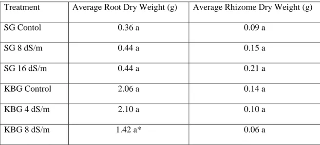
Table 1.1: Average Dry Weights of Roots and Rhizomes from In-growth root tubes. Letters indicate differences in mean separation test ...16
Table 2.1- Years planted and years sampled of field grown saltgrass. All stands grown at the Colorado State University Horticulture Research Center ...42
Table 2.2- Average Root Weights by depth for the 4 stand ages ...43
Table 2.3- Contrast of each stand age at every depth to find where significant separation between stands...44
vii
LIST OF FIGURES
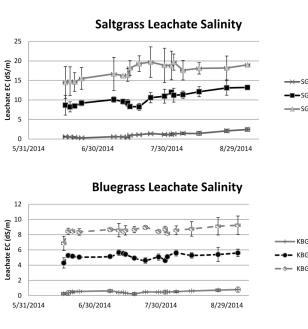
Figure 1.1 and 1.2 – Electrical conductivity of irrigation water leachate collection for Saltgrass (SG) and Kentucky bluegrass (KBG). Collections of leachate was made weekly to ensure proper salinity levels were maintained ...17
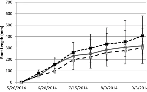
Figure 1.3 - Total Saltgrass Root Length (coarse and fine) Data was normalized to zero root
length at start of salinity (Salinity Treatments began on 6/1/2014) ...18
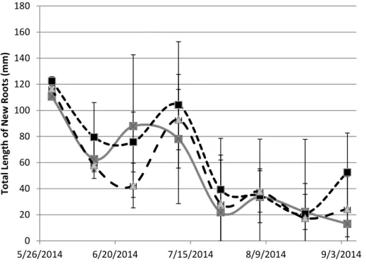
Figure 1.4: Average Net Length of saltgrass root growth (coarse and fine) produced at each measurement date after salinity treatments began. Includes all 4 pots of each treatment averaged together by treatments (n=12) over 8 measurement dates (5/30/2014 to 9/5/2014) ...19
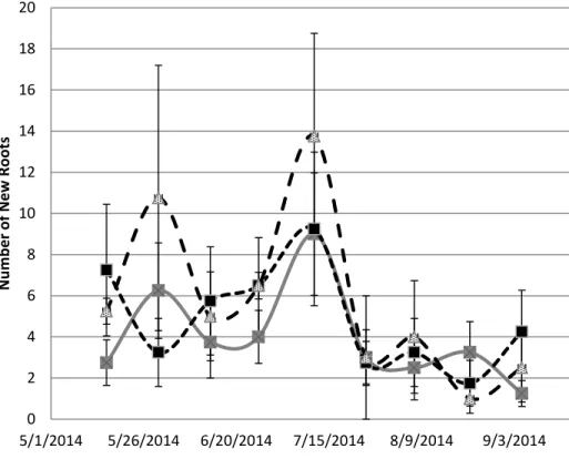
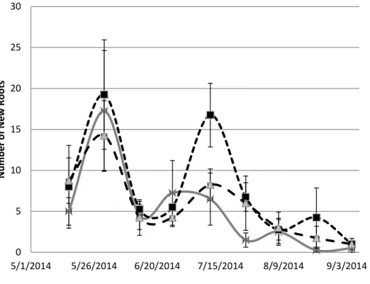
Figure 1.5 – Saltgrass Net Root Counts: Points are the number of roots (both fine and coarse) produced between each measurement date at upper depth (4cm) ...20
Figure 1.6- Saltgrass Net Root Counts: Points are the number of roots (both fine and coarse) produced between each measurement date at lower depth (15cm) ...21
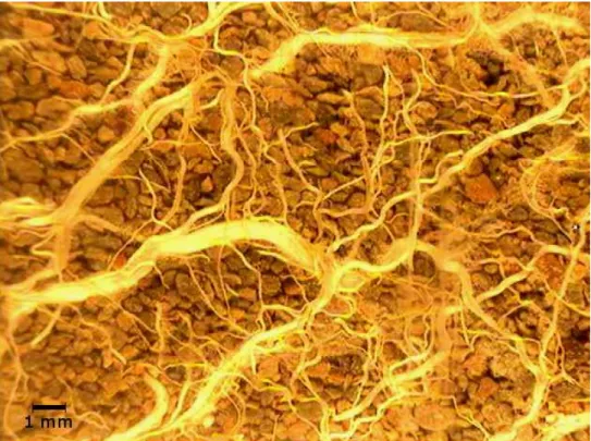
Figure 1.7 - Minirhizotron image showing different size orders of Saltgrass roots. Image from Pot #4 (8 dS/m) Depth 15cm taken on 8/22/2014...22
Figure 1.8- All traced saltgrass roots graphed in ascending order of increasing diameter. Root number is an arbitrary number assigned to each root when placing in ascending order ...23
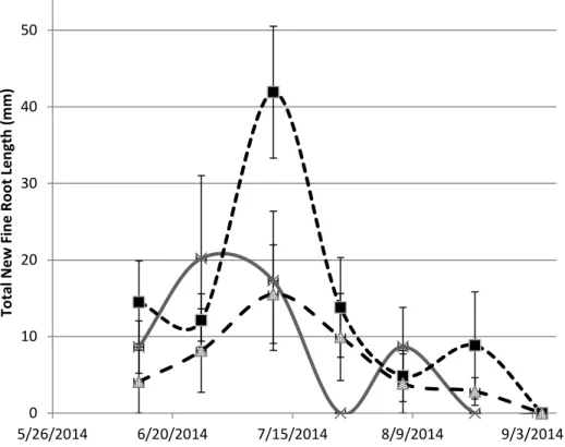
Figure 1.9- Saltgrass Net Fine Root (<0.25mm) growth at 15 cm depth after salinity treatment .24
viii
Figure 1.11- In growth tube with 9 2-inch diameter holes around the outside. Internal volume of 295 cm3. Covered in coarse mesh and refilled with fritted clay once placed into the cored out section of the pot. ...26
Figure 1.12 and 1.13: Average total weight for Saltgrass(SG) and Kentucky Bluegrass(KBG)of all roots and rhizomes produced in-growth root cores(295cm3) 4 pots of each treatment averaged together by treatments (n=12) ...27
Figure 1.14 and 1.15- Saltgrass (SG) and Kentucky Bluegrass(KBG) clipping dry weight(g) from biweekly mowing ...28
Figure 1.16 - Saltgrass Root length (RL) and shoot dry weight (SDW) ...29
Figure 1.17 - Turf Quality images taken from similar angles over the experiment just after
mowing and on the dates of minirhizotron image collection. Bluegrass at the top with TQ ratings of 9,8,6,4 (left to right) and saltgrass below with TQ ratings of 6,5,3,2 (left to right) ...30
Figure 1.18 and 1.19 – Turf Quality values over time for Saltgrass (SG) and Kentucky bluegrass (KBG). Turf Quality is a unitless subjective measure of visual characteristics of turfgrass ...31
Figure 2.1- Root Weight by Depth in soil cores of field grown saltgrass (SG) including Kentucky Bluegrass for comparison, (*) next to depth notes significant difference between stand ages at that sampling depth (P= 0.05) ...45
Figure 2.2 - Average root length visible at end of November 2014 from minirhizotron ...46
Figure 2.3- Minirhizotron net root length of saltgrass (SG) and Kentucky bluegrass (KBG) with Soil temperature at a depth of 15cm ...47
ix
Figure 2.4- Average root diameter of Saltgrass (SG) and Kentucky Bluegrass (KBG) from
1
CHAPTER 1: THE EFFECTS OF SALINITY ON ROOT GROWTH IN CONTAINER GROWN SALTGRASS AND KENTUCKY BLUEGRASS
SUMMARY
Soil salinity can affect soils in all climates but is particularly common in arid
environments and has numerous causes. Saline soils greatly reduce the growth of most plants we aim to grow. In this study the effects of salinity on root growth were examined in inland
Saltgrass (Distichlis spicata L. Greene). Kentucky Bluegrass (Poa pratensis L.) was examined for comparison. Quality and quantity of root growth has effects on the rest of the plant. When the roots are greatly reduced , either through die-back or reduced growth, then the shoot material will often also be suppressed or killed. The objective of this experiment was to to quantify the effects of salinity on inland saltgrass. A minirhizotron system was used to view root growth over time. In-growth root tubes were used to support minirhizotron data. Grasses were grown in pots within growth chambers and salinity was applied through irrigation water at levels of 8 and 16 dS/m. Shoot production and turf quality data was also collected. Salinity resulted in periodically increased fine root growth (flushes) and rhizome production within the 8 dS/m treatment in saltgrass. Increased fine root production greatly increases the root surface area for water and nutrient absorption. This has unknown implications for growth within a saline environment but may help with osmotic regulation. More research is needed to to understand the benefits of root flushing and increased surface area under saline conditions but changes in root growth appear to be an adaptive response to salinity stress.
2 INTRODUCTION
The arid West is a unique environment for plant growth. Water is often a limiting factor and with the arid environment comes other confounding factors like salinity. Rock weathering, high water tables, poor quality irrigation water, and de-icing salts all contribute to higher salinity levels in soils. There are few turf grasses that grow well in arid and saline environments. Saltgrass (Distichlis spicata L. Greene) is unique in its ability to grow in such environments.
Inland saltgrass is native to the Americas, Middle East, and Africa, where it is commonly found in salt flats or sea-shores (Gould, 1968; Pessarakli 2001). Saltgrass (SG) showed promise for development into good quality turfgrass with the following characteristics: tolerance to regular mowing and wear, compaction, and drought, which were the foci of the breeding program at Colorado State University (Hughes et al., 2002). Studies to examine physiological responses studied the effects of salinity on SG in hydroponics (Qian et al., 2007; Pessarakli et al. 2008; Pessarakli 2011). Root dry weights were also recorded either at the end of the experiment (Pessarakli et al. 2008, Pessarakli 2011) or at the end of a length of time at one salinity level (Qian et al., 2007) and at the end. In Pessarakli et al. 2008, total root system length was quantified as a measurement of the base of the shoots to the tips of the roots when the plants were removed from the solution. From those measurements it was found that root dry mass decreased in all treatments, 10, 20, and 40 dS/m. In Qian et al. 2007 and Pessarakli 2011 root dry mass increased up to 36 and 34 dS/m respectively but dry mass was reduced at levels beyond these levels. When salinity effects on the root system that will in turn have an effect on the whole plant. Yet these were hydroponic studies that lacked soil media that may have an effect on plant response to salinity. Root growth can be strongly affected by a growing media when compared to hydroponic studies (Snapp & Shennan, 1992). Snapp and Shennan found up to a
3
50% reduction in root growth of soil grown tomatoes under salinity stress compared to hydroponic salinity studies at similar levels of salinity. Quantifying root growth in soil is a difficult task due to the opaque nature of the growing media. Minirhizotron tubes have been used to observe root growth in a variety of plant species; wheat (Asseng et al., 1998), oats (Bragg et al., 1983), grapes (Comas et al., 2000), and hardwood forest (Hendrick & Pregitzer, 1992). Minirhizotron allows for repeated observation of root growth, within the soil, over the duration of the experiment.
Minirhizotron has been used to study a variety of turfgrass species root systems (Murphy et al., 1994; Liu & Huang 2001; Huang & Liu, 2001; Fu et al., 2007). Minirhizotron allows the observation of root growth over time for quantification of root length and measurements of root system architecture. Minirhizotron has been used to observe root growth of saltgrass and other grasses, growing together, for population ecology purposes (Snook & Day, 1995) but in that study roots of numerous species were observed together with no way to distinguish between the different species. The objective of this study is to observe the effects of salinity on root growth and architecture in soil grown plants. Minirhizotron was used to observe root growth of inland saltgrass and Kentucky bluegrass, under salinity stress, in order to more accurately measure root length changes from salinity and investigate changes in root system architecture that wasn’t possible in previous studies.
MATERIALS AND METHODS
In this experiment, saltgrass(SG) and Kentucky bluegrass(KBG) were grown in containers within separate growth chambers, each maintained at their optimal growing
4
temperatures. Salinity was imposed on the plants by irrigating with saline water. Soil salinity treatments (~0, 8, 16 dS/m for saltgrass and ~0, 4, 8 dS/m for Kentucky bluegrass) were arranged in a randomized complete block design within the growth chambers and treatments began once grasses were full established in the pots. Root growth was continuously monitored using minirhizotron technique, and in-growth soil cores were used to show differences in root growth over the length of the experiment.
Plant materials and growth conditions
Saltgrass seedswere collected from experimental lines developed at Colorado State University. Seeds were winnowed, cleaned, and cold stratified for twenty-eight days at 4ºC to help increase germination. KBG variety used in this experiment was NuGlade, which is a common variety of KBG used on golf courses. Pots were 15 liters (Polytainer, #5 squat) and were filled with greens grade Turface (Profile Products llc, Buffalo Grove, Ill.), which is
comprised of 100% fritted clay. Turface was used because it is good for water retention and has a moderate cation exchange capacity of 33.6 mEq/100g . Seeding rates were 730g per for
bluegrass and 980g per 100 m2 for saltgrass. Although seeding rate was higher in the SG, KBG has a smaller seed which, at the same rate, would result in a greater seeding density in the bluegrass compared to saltgrass. All pots were covered with permeable agriculutural nonwoven fabric cloth or horticultural row cover cloth to hold in moisture and were misted three times a day until seedlings were rooted. Grasses were grown for 4 months watered with DI water and fertilized with 17 kg/ha N every watering (4 times a week) for the length of the experiment (Gro-More 20-20-20). The 4 month growing period allowed full establishment of grasses in the pots until a uniform turf covered the at least 80% of the surface in both grasses.
5
Seeded SG and KBG were grown in separate growth chambers each under their optimal growing conditions. Growth chambers were used for this experiment because they provide a stable growing environment over the many months of observation. The growth chambers (Conviron PGR15) were 0.5m by 1.5m by 1.5m in dimension and PAR was 875 μmoles/m²/s. Temperatures were 25°C and 36.5°C in the day time and 14°C and 21.5°C in the night for KBG and SG respectively. Relative humidity was set at 75% during the day and 50% at night for both chambers and day length was 13 hours. Grasses were mowed every other week to a height of 3 inches. Plants were rotated every week to help reduce temperature and moisture gradients present in the growth chambers.
Minirhizotron
Minirhizotron tubes were made of acrylic. One layer of black pipe wrap and one of white electrical tape were added to the exposed top of the tube that extended up from the soil in order to exclude light, which could affect root growth. The top of the tubes were plugged with a stopper and covered with an aluminum cap. The tubes were secured into place at the top edge of the pot and passed diagonally from the top edge to the opposite bottom corner at an angle of 30° from vertical. The viewing area of the minirhizotron tube in each pot was oriented parallel to the soil surface and to view the same side of the pot. Tubes had seventeen centimeters long viewing area resulting in fifteen centimeters of soil depth viewable once the angle of the tube was
accounted for. The viewing area of each window analysed was 3.3cm2.
Minirhizotron images were collected biweekly from the first signs of germination. Images were analyzed for root length using Rootfly software (ver. 9.2.1, Clemson, 2001). Due to the images being very densely packed with roots, two images per tube were analyzed at soil
6
depths of four and fifteen centimeters below soil surface. Roots were eventually analyzed in two separate size types. A diameter of 0.25 mm was used for separation of roots into fine and coarse root orders.
Soil Salinity
Salinity was introduced after the stand establishment period (four months) and was added to the pots through irrigation water. Salts used were ocean salts (Instant Ocean-Supplemental Data 1.1) and irrigation water salinity levels were set at half of the objective soil salinity with a 0.5 leaching fraction. To achieve a soil salinity of 4 dS/m, for example, the irrigation water was set at 2 dS/m and half of the irrigation water applied was allowed to pass through the pot and drain out. Leaching fraction was calculated by FAO equation (Ayers & Westcot, 1985).
����ℎ��� �������� (��) =����ℎ �� ����� ����ℎ�� ����� �ℎ� ���� ����
����ℎ �� ����� ������� �� �ℎ� �������
Allowing half of the water applied to pass through the pots assisted in achieving uniform salinity distribution through the pots and ensured all pots were fully watered with each irrigation. Pots were watered every Sunday, Monday, Wednesday and Friday on a uniform weekly schedule. Salinity treatments were eight and sixteen dS/m in SG and four and eight dS/m in KBG, both contained a control of only DI water application. All treatments, including control, continued to be fertilized with 17 kg/ha N every week (GrowMore 20-20-20) during salinity treatments. Soil salinity was measured by collecting irrigation leachate and measuring it for electrical
conductivity (E.C.) with an Accumet AP75 conductivity meter. Soil salinity is similar to the leachate passing from the root zone. Leachate was collected weekly during the Sunday watering to confirm salinity levels through the duration of the experiment (Figure 1.17). Salinity levels used were chosen because they are comparable to salinity levels that maybe found in field
7
growing conditions. Different salinity levels were used for the two grasses because Kentucky bluegrass doesn’t tolerate salt as well as saltgrass and therefore had lower treatment levels to obtain similar stress.
In-growth cores
In-growth cores were used to determine the root length produced per soil volume of each species and treatment during the salinity treatments. The cores were made from two inch PVC that was fifteen cm long. This resulted in a volume of 295 cm3. The tube had nine 2-inch diameter holes drilled around the outside and was covered with coarse mesh (1-2mm openings) (Figure 1.9). The in-growth cores were packed with fresh fritted clay and inserted where a core of the same volume of soil was removed, opposite the minirhizotron viewing area. One core was installed in each pot just prior to the beginning of salinity treatments. In-growth tubes remained in the pots until the experiment was terminated (95 days). Roots and rhizomes were washed free of soil, separated, oven dried at 65° C and weighed.
Shoot Biomass
All pots were mowed to a height of 7.50 centimeters every other week on the same day that minirhizotron images were captured. Grass clippings were collect with a wet/dry vacuum that had a mesh bag on the collection end of the suction hose. This allowed even small blades of grass to be collected quickly and easily. Each pot’s clippings were collected individually. The clippings were then oven dried at 65°C for 48 hours and weighed.
8 Turf Quality
Turf Quality (TQ) was quantified for all the pots over the duration of the salinity treatments. Turf quality is a subjective assessment based mainly on visual variables related to quality and health . National Turfgrass Evaluation Program has guidelines to evaluate the texture, ground cover, density, viability/health and color (Morris & Shearman, 2010). The
texture, ground cover, and density did not vary between the treatments and is primarily useful for comparing among turfgrass species or hybrids. Turf quality in response to salinity was assessed in this experiment by turf color and health of the shoots. For color, the scale was from one to nine with one being straw colored and nine being a deep rich green. The measure of health was grouped into color for this experiment as a decrease plant health was assumed to be the reason behind the yellowing or lightening from the plants normal genetic color. Turf quality baselines were different for the two species of grasses with saltgrass starting at a six due to its lighter color and bluegrass starting at an eight due to its deep green color (see figure # for example photos). In an attempt to remove variation among assessments, images were taken from a similar angle and orientation of the pots every other week just after the grasses were mowed. At the end of the experiment, all the images were analyzed at once. A TQ image analysis scale was formed for each grass comparing side by side images of different TQ ratings. This scale was used for comparison during quantification of TQ from remaining photos.
Statistical Design and Analysis
Treatments were assigned by dividing twelve pots into four groups depending on percent coverage of shoots and then randomly assigned treatments within those 4 groups. Pots were arranged in a randomized complete block design. Root growth in minirhizotron window, turf
9
quality, shoot biomass from biweekly clippings, and root biomass from root in-growth cores were analyzed using PROC MIXED (SAS 9.4, SAS Institute,Cary, NC). The response variable for minirhizotron was root length, net root counts or root surface area. Fixed effects included treatment (control, 8dS/m, 16dS/m), depth of observation (4cm and 15cm). Pot nested within treatment was included as a random effect to account for repeated measures.
RESULTS AND DISCUSSION
Soil Salinity
Soil salinity, as measured by electrical conductivity of leachate, increased slightly and insignificantly over time in both saltgrass and Kentucky bluegrass (Figure 1.1 and 1.2). Despite the slight temporal differences, soil EC differed between salinity treatments throughout the duration of this experiment. The average leachate EC for the salinity
treatments in saltgrass was 1.0, 10.3, and 17.4 dS/m for salinity treatments with targets of 0, 8, and 16 dS/m,respectively. In Kentucky bluegrass, EC for the salinity treatments was 0.5, 5.2, and 8.5 dS/m for targeted salinity of 0, 4,and 8 dS/m, respectively.
Root Growth in Minirhizotron Viewing Areas
Root growth was examined over a 8 month period, including a 4 month period of stand establishment and 4 month period after treatments were initiated. Bluegrass roots were very fine and grew densely, root growth in bluegrass images after one month was impossible to track. Thus, Kentucky bluegrass images were not analyzed for root growth. After the 4 month establishment period the rate of root growth slowed and root growth in all pots was consistant
10
before treatments began (Figure 1.3). Total new root production, the total length produced between viewing dates, occurred in periodic increases in root growth rates followed by decreased growth rates, which all pots experienced regardless of treatment. Root growth in minirhizotron viewing areas fluctuated between 40-120 mm of root length per viewing area (Figure 1.4). New root length production in minirhizotron viewing areas had no significant separation between the treatments (P=0.6948). It is not clear why root production occured in a non-constant rate. Gallagher et al. (1984) found that fluctuations in sugar and carbohydrate concentrations were correlated with root and rhizome production in another salt marsh species, Spartina alterniflora, but this was tied to seasonal variation in plant growth, which did not occur in the controlled environment of growth chambers. New root length production was also
analyzed at each depth, 4 and 15 cm, in each pot (P= 0.707 at 4cm and P= 0.6175 at 15 cm) (Figure 1.5 and 1.6). Next pots were analyzed for the count of new roots produced. Net root counts had corresponding increases and decreases at the same dates as length, this is expected as this is just another measurement of growth. Within the viewing areas a period of rapid growth would add 25 roots produced and at other times no viewable roots would be produced between image collection sessions. There was a period of root flush about a month and a half after salinity began, on 7/13/2014, that occurred in both upper and lower viewing areas. In the lower viewing areas only the 8 dS/m treatment had increased growth with the control and 16 dS/m treatments not having increased growth. This showed close to significant results (P = 0.1567).
When analyzing minirhizotron images two distinct sizes of roots can be seen on the recorded images (Figure 1.7). The two classes of roots would serve different purposes to the plant. Smaller diameter roots have a greater surface area to volume ratio and are much more effiecnt at water uptake. Larger diameter roots conduct water to the shoots from the smaller
11
diameter absorbing roots. With salinity effecting the osmotic gradient of water uptake there was a possibility that root production was shifting towards increased numbers of fine roots produced to increase water uptake. At this point all root diameters were ordered by increasing diameter and graphed to visualize what cut off point should be for separation of root orders (Figure 1.8). The value that was selected to separate the orders was 0.25 mm. Any roots that were < 0.25 mm was considered fine roots and anything greater were considered coarse roots. The 0.25mm separation point was chosen due to the fact that most roots seen in minirhizotron images were fine roots then there was a distinct and large difference in diameter up to coarse roots. In figure 1.8, 0.25mm corresponds to the point at which most roots are smaller than but also roots above 0.25mm drastically begin to increase in diameter. From this it seemed like a logical dividing line between fine and coarse root classes.
There was a spike in fine root growth at the 15 cm observation depth in the 8 dS/m treatment that wasn’t present in either the control or the 16 dS/m (P = 0.0264). A fine root flush resulted in a greater surface area for absorption (Figure 1.10). Previous studies found decreasing length with increasing salinity levels, 0, 10, 20, and 40 dS/m (Pessarakli et al., 2008). In Pessarakli et al. 2008, a decrease in root growth began 6 weeks after the initiation of salinity treatments. In this study there was a non-significant increase in root length after salinity began in the 8 dS/m but no increase at all in the 16 dS/m (Figure 1.3). It is difficult to compare our results to Pessarakli et al. 2008 as they measured the whole root system length when removed from hydroponic solution, whereas minirhizotron only allows a small window of observation. Yet interestingly the significant results came in about the same timeframe, c. 6 weeks after salinity began. This may accurately represent the timeframe for seeing ionic effects of sodium buildup in saltgrass (Munns, 1986). In this study the significant effects of salinity were in fine
12
root flushes at the 15 cm level in 8 dS/m. It is difficult to say why a significant fine root flush only occurred at 8 dS/m and at 15cm depth. One possible explaination is that being a halophyte saltgrass grows more optimally at moderate salinity levels and the fine root flush enables increased water uptake to supply the increased water demand from the roots. This is probably not the case as there wasn’t a significant increase in shoot clipping dry weights following the fine root flush. Another possible reason is that an increase in fine roots is a responsive change to external conditions. Increases in fine root production have been found in many plant species in response to various environmental changes (Lynch, 1995; Lopez-Bucio et al., 2003; Malamy 2005; Ostonen et al.,2007).
In-growth root tubes
Salinity had opposite effects on trends between saltgrass (SG) and Kentucky bluegrass (KBG) in respect to rhizome growth (Figure 1.12). Root growth increased slightly with increasing salinity in saltgrass. There was a 0.08g increase in the 8 dS/m treatment when compared to the control and little to no increase between the 8 and 16 dS/m treatments. The opposite was true for the root growth of Kentucky bluegrass. There was a 0.04g increase in the average of the 4 dS/m treatment when compared to the control. Then there was a large 0.68g decrease from the 4 dS/m to the 8 dS/m treatments. This was the most sizable change in root dry weight and was marginally significant (P= 0.0898). The trends in root dry weight among the two grasses were expected. Saltgrass has shown increased root dry weights in response to
salinity up to ~34 dS/m in previous studies (Qian et al., 2007; Pessarakli 2011). KBG showed a 50% decrease in root dry weights at salinity levels of 2.2 and 9.2 dS/m and 5.8, 19.6, 24.9 and 41.0 dS/m resepectively (Qian et al.,2001; Alshammary et al., 2004).
13
Rhizomes dry weights also followed a similar trend between the two grasses. Saltgrass trended towards greater dry weight with increasing salinity. Saltgrass rhizome dry weights are as follows with 0.085g in the control, 0.147 at 8 dS/m, and 0.2072 at 16 dS/m (Figure 1.12). Bluegrass had a very slight decrease from a high of 0.139g in the control, 0.097 in 4 dS/m, and a low of 0.064g in 16 dS/m (Figure 1.13). In-growth root cores were used to both draw parallels to previous research that measured root system response to salinity and also to validate
minirhizotron quantification of root growth. The findings of this paper are in agreement with previous studies.
Shoot Biomass
Leaf biomass collected from clippings fluctuated during the experiment with periods of higher and lower growth (Figure 1.14 and 1.15). Statistical analysis yielded no significant effects of treatment for either saltgrass (P=0.2352) or Kentucky bluegrass (P = 0.8816). As the root length production decreased after about two months of salinity treatments, the shoot dry weights increased (Figure 1.16). Salinity stress has been shown to suppress shoot growth and increase root growth (Munns and Termaat, 1986). This occurred early in the salinity treatments but reversed as treatments continued. Measurements of leaf area in addition to leaf dry weight would have been helpful in this experiment. Leaf area to leaf dry weight ratio could have shown that increases or decreases in weights were from shoot elongation and not other factors such as solute accumulation or leaf thicking.
Turf Quality
Turf Quality (TQ) was assessed at the end of the experiment from pictures that were taken at two week intervals after grasses were mowed. Saltgrass was given a baseline turf
14
quality value of 6 and bluegrass a baseline of 8. This was representative of the average TQ of the grasses before the salinity treatments began. The TQ ratings of both grass species rose and fell during the salinity treatments, including the control, the greater the salinity the steeper the drops and the less of a recovery when rising again. A TQ rating of 4 was the considered
unacceptable in the TQ assessment, this value was also used in other studies of grass evaluation (Pessarakli et al., 2008; Qian et al.,2007). Saltgrass had a lower baseline value due to its lighter green genetic leaf color which is less desirable characteristic according to the National Turfgrass Evaluation Program (Morris & Sherman, 2010) (Figure 1.17). The base of saltgrass tended to loose green color and become straw colored after the shoots were mowed. Shoots were still viable and continued to produce new green leaves but were straw colored below the normal mowing height of 3 inches. Yellowing of the shoots was the same for the treated and untreated grasses, this lead to a steady decline in TQ for all saltgrass, regardless of treatment, over time (Figure 1.19). Hughes et al. mentioned “browning” of some of the saltgrass lines after mowing (Hughes et al., 2002). Other salinity studies didn’t report browning after mowing but were using different saltgrass lines (Pessarakli et al., 2008; Qian et al.,2007). Saltgrass began at a baseline of 6 and dropped from the beginning of the experiment. Only one of the 8 dS/m treatment pots fell below the unacceptable rating of 4 and 3 of the 4 pots in the 16 dS/m treatment fell below a TQ rating of 4. Saltgrass overall had an average of 5 for the TQ rating, this was mainly due to the yellowing of the lower shoots after mowing. With all treatments having reduced TQ over time the effects of salinity did not impact TQ in saltgrass (P= 0.8591).
Salinity stress caused Kentucky bluegrass to lighten and began to die from the middle of the pot to the edge in the higher treatments. Within a month the effects of salinity on TQ were evident in bluegrass. In the 4 dS/m TQ ratings fell from a high of 8 to a low of 6.4. The 8 dS/m
15
treatment quickly declined in the first month of salinity treatments to a rating of 6. Then slowly declined to the end of the experiment to an average of 5.8 (See Figure 1.18). Bluegrass is very susceptible to salinity stress resulting in significant differences in treatments (P= 0.0054). Alshammary et al. found similar results in both bluegrass and saltgrass, in their hydroponics study, KBG reduced from TQ rating of 9 in control to 6 at 4.81 dS/m and 4 at 9.4 dS/m. Saltgrass began with TQ of 5 and only dropped to 4 at salinity above 18 dS/m (Alshammary et al., 2004).
CONCLUSION
Saltgrass grows well in a saline environment. In this experiment we used lower salinity levels than previous experiments with saltgrass (Gessler, N. & Pessarakli, M. 2009, Pessarakli, M. et al. 2008.) Salinity at 8 dS/m increased in fine root production, which could have
implications for water uptake by increasing the total absorbing surface area. Biomass of roots and rhizomes from in-growth soil cores had a slight increase between the control and salinity treatments but there was little difference between the 8 and 16 dS/m treatment. The increase root biomass weight may also have been due to increased fine root production but the roots weren’t separated before drying and weighing. Turf quality had almost no differences between the highest level of treatment and the control.
16 TABLES
Table 1.1: Average Dry Weights of Roots and Rhizomes from In-growth root tubes. Letters indicate differences in mean separation test. *KBG 8dS/m was maginally separated (P= 0.0898). Treatment Average Root Dry Weight (g) Average Rhizome Dry Weight (g)
SG Contol 0.36 a 0.09 a SG 8 dS/m 0.44 a 0.15 a SG 16 dS/m 0.44 a 0.21 a KBG Control 2.06 a 0.14 a KBG 4 dS/m 2.10 a 0.10 a KBG 8 dS/m 1.42 a* 0.06 a
17 FIGURES
Figure 1.1 and 1.2 – Electrical conductivity of irrigation water leachate collection for Saltgrass (SG) and Kentucky bluegrass (KBG). Collections of leachate was made weekly to ensure proper salinity levels were maintained. Error bars represent standard error.
0 5 10 15 20 25 5/31/2014 6/30/2014 7/30/2014 8/29/2014 Lea ch a te E C ( d S /m )
Saltgrass Leachate Salinity
SG Control SG 8 dS/m SG 16 dS/m 0 2 4 6 8 10 12 5/31/2014 6/30/2014 7/30/2014 8/29/2014 Lea ch a te E C ( d S /m )
Bluegrass Leachate Salinity
KBG Control KBG 4 dS/m KBG 8 dS/m
18
Figure 1.3 - Total Saltgrass Root Length (coarse and fine) Data was normalized to zero root length at start of salinity (Salinity Treatments began on 6/1/2014). Error bars represent standard error. 0 100 200 300 400 500 600 700 5/26/2014 6/20/2014 7/15/2014 8/9/2014 9/3/2014 Ro o t L en g th ( m m ) SG Control SG 8 dS/m SG 16 dS/m
19
Figure 1.4: Average Net Length of saltgrass root growth (coarse and fine) produced at each measurement date after salinity treatments began. Includes all 4 pots of each treatment averaged together by treatments (n=12) over 8 measurement dates (5/30/2014 to 9/5/2014).
0 20 40 60 80 100 120 140 160 180 5/26/2014 6/20/2014 7/15/2014 8/9/2014 9/3/2014 T o ta l L en g th o f N ew Ro o ts ( m m ) SG Control SG 8 dS/m SG 16 dS/m
20
Figure 1.5 – Saltgrass Net Root Counts: Points are the number of roots (both fine and coarse) produced between each measurement date at upper depth (4cm) Error bars represent standard error. 0 2 4 6 8 10 12 14 16 18 20 5/1/2014 5/26/2014 6/20/2014 7/15/2014 8/9/2014 9/3/2014 N u m b er o f N ew Ro o ts Control 8 dS/m 16 dS/m
21
Figure 1.6- Saltgrass Net Root Counts: Points are the number of roots (both fine and coarse) produced between each measurement date at lower depth (15cm). Error bars represent standard error. 0 5 10 15 20 25 30 5/1/2014 5/26/2014 6/20/2014 7/15/2014 8/9/2014 9/3/2014 N u m b er o f N ew Ro o ts Control 8 dS/m 16 dS/m
22
Figure 1.7 - Minirhizotron image showing different size orders of Saltgrass roots. Image from Pot #4 (8 dS/m) Depth 15cm taken on 8/22/2014.
23
Figure 1.8- All traced saltgrass roots graphed in ascending order of increasing diameter. Root number is an arbitrary number assigned to each root when placing in ascending order.
0 0.2 0.4 0.6 0.8 1 1.2 0 500 1000 1500 2000 2500 Ro o t D ia m et er ( m m ) Root Number Root Diameter
24
Figure 1.9- Saltgrass Net Fine Root (<0.25mm) growth at 15 cm depth after salinity treatment. Error bars represent standard error.
0 10 20 30 40 50 5/26/2014 6/20/2014 7/15/2014 8/9/2014 9/3/2014 T o ta l N ew F in e Ro o t Len g th ( m m ) SG Control SG 8 dS/m SG 16 dS/m
25
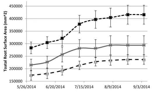
Figure 1.10- Saltgrass Fine Root surface area. Error bars represent standard error.
150000 200000 250000 300000 350000 400000 450000 5/26/2014 6/20/2014 7/15/2014 8/9/2014 9/3/2014 T o a ta l Ro o t S u rf a ce A rea ( m m ^ 2 ) SG Control SG 8 dS/m SG 16 dS/m
26
Figure 1.11- In growth tube with 9 2-inch diameter holes around the outside. Internal volume of 295 cm3. Covered in coarse mesh and refilled with fritted clay once placed into the cored out section of the pot.
27 0 0.1 0.2 0.3 0.4 0.5 0.6 SG Control SG 8 dS/m SG 16 dS/m W e igh t ( g) SG Roots SG Rhizomes
Figure 1.12 and 1.13: Average total weight for Saltgrass(SG) and Kentucky Bluegrass(KBG)of all roots and rhizomes produced in-growth root cores(295cm3) 4 pots of each treatment averaged together by treatments (n=12). Error bars represent standard error.
0 0.5 1 1.5 2 2.5 3 KBG Control KBG 4 dS/m KBG 8 dS/m W e igh t ( g) KBG Roots KBG Rhizomes
28
Figure 1.14 and 1.15- Saltgrass (SG) and Kentucky Bluegrass(KBG) clipping dry weight(g) from biweekly mowing. Error bars represent standard error.
0 1 2 3 4 5 6 7 8 9 10 5/26/2014 6/20/2014 7/15/2014 8/9/2014 9/3/2014 C li p p in g Dr y W e igh ts ( g) SG Control SG 8 dS/m SG 16 dS/m 0 1 2 3 4 5 6 7 8 9 5/26/2014 6/20/2014 7/15/2014 8/9/2014 9/3/2014 C li p p in g Dr y W e igh ts ( g) KBG Control KBG 4 dS/m KBG 8 dS/m
29
Figure 1.16 - Saltgrass Root length (RL) and shoot dry weight (SDW). Error bars represent standard error. 0 1 2 3 4 5 6 7 8 9 10 0 20 40 60 80 100 120 140 160 180 5/26/2014 6/20/2014 7/15/2014 8/9/2014 9/3/2014 S h o o t D ry W e igh ts ( g) Ro o t L en th ( m m ) RL-Control RL-8 dS/m RL-16 dS/m SDW-Control SDW-8 dS/m SDW-16 dS/m
30
Figure 1.17 - Turf Quality images taken from similar angles over the experiment just after
mowing and on the dates of minirhizotron image collection. Bluegrass at the top with TQ ratings of 9,8,6,4 (left to right) and saltgrass below with TQ ratings of 6,5,3,2 (left to right).
31
Figure 1.18 and 1.19 – Turf Quality values over time for Saltgrass (SG) and Kentucky bluegrass (KBG). Turf Quality is a unitless subjective measure of visual characteristics of turfgrass. Error bars represent standard error.
4 5 6 7 8 9 10 5/31/2014 6/25/2014 7/20/2014 8/14/2014 9/8/2014 T u rf Q u a li ty R a ti n g KBG Control KBG 4 dS/m KBG 8 dS/m 3 4 5 6 7 5/31/2014 6/25/2014 7/20/2014 8/14/2014 9/8/2014 T u rf Q u a li ty R a ti n g SG Control SG 8 dS/m SG 16 dS/m
32
CHAPTER 2: ROOTING DEPTH AND ROOT GROWTH OF FIELD GROWN SALTGRASS AND BLUEGRASS
SUMMARY
Field observations of root growth are difficult due to the opaque nature of soil but important because spatial distribution and timing of root growth has a profound effect on the above ground growth. In this study, root growth of field grown saltgrass was studied with minirhizotron and soil coring techniques to better understand root system development with stand age.
Minirhiozotron techniques allow root growth to be studied over time. Soil coring was used to examine root distributions deeper than possible with minirhizotrons. Saltgrass had two flushes of root growth. The first occurred earlier in the season than expected, months before shoot growth. The second and larger flush of root growth coincided with the onset of shoot growth above ground. Maximum root depth in saltgrass was found in four year old stand with roots reaching 270 cm down the soil profile. The deep rooting of saltgrass maybe responsible for increase drought tolerance exhibited in earlier studies. Saltgrass is certainly a unique species of grass that warrants more research and may hold valuable attributes that could be used where other turfgrasses fall short.
INTRODUCTION
The use of municipal water to irrigate turfgrass is under increased scrutiny due to competeing interest in this precious resource. Native grasses have the potential to occupy a niche in the
33
turfgrass market because they have lower mowing, fertilization, and watering requirements (Mintenko, 1999). Lower irrigation water requirements of native grasses could from a
combination of reduced evapotranspiration( ET) and deeper roots within the soil, which are able to acquire deep water reserves that are out of reach of other plants. In this study we look at root growth and rooting depth of a native grass commonly called saltgrass and how the depth could effect water uptake. Saltgrass (Distichlis spicata L. Greene) is a species, native to North America that has been bred and selected for turf characteristics at Colorado State University. Evapotranspiration (ET) data on saltgrass show it using an average of 4 mm of water a day during the warm summer months when ET rates are highest. This is roughly half the ET of other warm season turfgrass species, such as Seashore paspalum and Zoysiagrass that average 7.0 to 8.5 mm/day (Kopec, 2004), and less than half of cool season turfgrasses, such as Kentuky Bluegrass and Fescue that use >10mm/day (Beard & Kim, 1989). During drought conditions saltgrass remained green and flowering when other native grasses, such as buffalograss and blue grama, which also have low ET, ~6-7 mm/day, were brown and dormant, suggesting that
saltgrass is more drought tolerant compared to other turfgrasses (Hughes et al., 2002). .
Root traits could explain how saltgrass is remaining green and flowering while other low water use grasses are dormant due to drought conditions. Drought tolerance would suggest that saltgrass can withstand periodic drought whereas drought avoidance means that the plant isn’t experiencing the drought other plants around it. Drought avoidance can be achieved by either completing life cycles when water is available, which is not applicable for perennial saltgrass, or by tapping into deep water reserves that may be out of reach of other plants. Grasses native to the American west, like inland saltgrass, are very often more deeply rooted than the conventional
34
profile was sufficient to meet their water requirements, these deep rooted grasses could reduce overall irrigation need and potentially allow for lawn management without irrigation in the arid Western US. These deeper rooting species may hold soil in place better than shallow rooting species (Brown et al. 2010). An issue with the use of native grasses is that they are often slow to establish, have a high rate of seed shatter, and cannot out- compete weeds as well as more
densely growing turfgrass (Brown et al. 2010). All of these factors make native grasses difficult to use commercially for both seed production and residential use. When the demand is large enough for the desirable traits only then will native grasses become more common place. In this study minirhizotron and soil coring were used to investigate root growth and rooting depth of field grown saltgrass, Kentucky bluegrass was used as a comparison species.
MATERIALS AND METHODS
Plant material and site information
Plots were located at the Colorado State Horticultural Field Research Center, seven miles northeast of Fort Collins, Colorado. All saltgrass plots were sprigged or seeded with
experimental line of turf-type saltgrass developed at CSU. Kentucky bluegrass was seeded in 2002 with NuGlade variety from Jacklin seed (Simplot, Boise, ID). Plots were established in different years between 2000 and 2012. Each age stand had at least 3 replicated plots. The soil type was Nunn clay loam (Aridic Argiustolls). There is no slope to the plots. Grasses were maintained under well water irrigation and mowed twice a week during the growing season to a height of two and half inches. The plots received an average 40.8 cm of rain per year and on average the frost-free growing season lasts from May 20 to September 20. Plots receive
35
supplemental irrigation of 4 cm weekly from June 1 to the middle of September. There is no hard pan or restrictive feature in the soil, although soil texture varies with depth.
Soil Coring
Root cores were taken in different years from plots with different age stands (Table 2.1). A soil core was collected from each plot down to 270 cm or until cores contained no roots. Sampling was completed using a 5 cm coring bit on a Giddings soil sampling machine
(Giddings,15SC/ Model GSRPS). Samples were separated into 30 cm long sections until final depth was reached. Samples were placed in a cooler upon sampling and then frozen until the roots were washed free of the soil. Subsamples were taken from random samples and scanned in to images which were analyzed for root length using DT-SCAN software. All samples were dried at 65C for 48 hours or until dry and were weighed for total dry root mass per sample. All of the root soil sampling was carried out during September to October . (Table 2.1). Previous data from bluegrass soil coring was also made available and was used in graphs of total rooting depth for visual comparison only. No statistical analysis was performed on the bluegrass data.
Minirhizotron
Six saltgrass plots (consisted of 2 lines with three replications) were seeded in spring of 2012. Minirhiztron tubes were installed on October 31, 2013. Concurrently, three minirhiztron tubes were installed in three Kentucky bluegrass plots for comparison. Fifty centimeter tubes were installed on a 30 degree angle from vertical to a depth of 43 cm. Individual images, 2.5 cm2, were captured in succession down the length of the tube. Images were collected beginning the week after installation, and then every 2 weeks during active growth periods (March to October) and monthly during winter dormancy (late October to early March). Images were
36
analyzed using Rootfly software (ver 9.2.1, Clemson Univ.). New root length produced in every other window was measured across all of the dates recorded (18 dates total).
Meteorological Data
Soil temperature at 15 cm was collected 1 mile north of the grass plots at a COAGMET station (FTC03) with a CSI Model 107 Soil Temp Probe and data collection on a Campbell Scientific CR10 data logger. This station is located at the same elevation, slope, and soil type as the research plots.
Statistical Design and Analysis
Data tables were arranged using Microsoft Excel and SAS 9.4 was used for statistical analysis. Minirhizotron and soil coring data was analyzed using PROC MIXED (SAS 9.4, SAS Institute,Cary, NC). The response variable for minirhizotron was root length, count or surface area. Fixed effects included plot and depth of observation. Minirhizotron tube nested within plot was included as a random effect to account for repeated measures.
RESULTS AND DISCUSSION
Soil Coring
Four year old saltgrass plots produced roots down to a depth of 240 cm. The root mass was greater with increasing age at each depth observed down to 150cm (Figure 2.1). Within the four different stand ages the largest separation in root dry mass produced occurred in the upper 30 cm with the eight year old stand having 250 mg more root dry mass than the five year old stand and 350 mg more root dry weight than the four and one year old stands. From 30 cm down
37
to 90 cm the 8 year old stand had greater dry root mass than the 1, 4, and 5 year aged stands from about 100mg greater from 30-60cm. Past 90 cm there was very little separation between the 8, 5, and 4 year old stands. By the 90-120cm depth interval the 1 year old stand had dropped to almost 0. At 120-150 cm the 1 year old stand had no roots present. 8 year old stand had a slight increase when compared to the 90-120 depth section (Figure 2.1 and Table 2.2).
Significant separations in stand age were further examined by a mean separation test to find which stands had significantly larger root weights (Table 2.3). 4, 5, and 8 year old saltgrass had similar root dry mass at depths deeper than 150 cm. However, this resulted in a statistically significant interaction between age of the stand and the depth sampled, meaning that the dry mass of the roots depends on the depth sampled.
In neighboring plots, Kentucky bluegrass had most roots in the top 30 cm and a sharp decline in root production with soil depth with no roots found deeper than 60 cm. These rooting patterns matched previous data (unpublished data, Qian 2005), and were consistent with values found in the literature (Wu, 1985, Weaver, 1926).
Saltgrass produces roots down to 270 cm after 4 years of growth. This is very deep rooting compared to most other species of turfgrass. Deep rooting in saltgrass may allow it to tap into groundwater within several meters from the soil surface. A rooting depth of 270 cm found for saltgrass in this study is the deepest observed to date. Deep-rooting in saltgrass
appears obligatory with findings of roots down to 42.5 cm, even when the groundwater was only 15 cm below the soil surface (Prodgers et al., 1991; Cooke et al., 1993). Inconsistent with findings here, Sevostianova et al. 2011 found no saltgrass roots below 60 cm in 1-2 year old stands of saltgrass grown in Arizona. More research is needed to identify the deepest extent of
38
saltgrass root penetration into the soil. However, the rooting depth found for saltgrass in this study has implications in its use as an alternative for more commonly grown turfgrass species.
Deep rooting is a common strategy for drought avoidance amongst plants native to an arid environment (Weaver &Albertson 1943; Canadell et al.,1996, Schenk & Jackson, 2002). When the soil close to the surface begins to dry from lack of rainfall and external competition from other plants deep rooted plants can access water that is out of reach of shallower rooting species. Irrigation managers could use the deep rooted nature of saltgrass to water deep and infrequently. This deep watering would allow the mature stand of saltgrass to acquire water needed to meet demand but when the water is used up from the upper soil profile weed competition and surface evaporation would be reduced due to lack of water.
It maybe specialized physiological mechinisms that allow saltgrass to reach depths of 270cm. In a non-saturated soil saltgrass can be very deep rooted and is comparable to other prairie species, including forbs and grasses, that have an average rooting depth of 1.2 to 2.4m (Weaver, 1968, Risser et al, 1981). In saturated soil saltgrass extends 30-40 cm below water table where low oxygen levels would be an issue (Cook et al.,1993; McNease, 1967). Saltgrass has aerenchyma cells in the roots which allow the diffusion of oxygen from higher up in the soil profile (Hansen et al.,1976). This marsh adaptation may carry over into deep rooting in non-saturated soil allowing roots to grow into areas were lower soil oxygen may limit the growth of other plants roots.
Root growth in minirhizotron viewing areas
Root growth by depth in the minirhizotron is similar to results from soil coring in that saltgrass had about half the root length as bluegrass in the top 20cm (Figure 2.2). Saltgrass had
39
an average of 200 mm per viewing window of total root growth from 0-10 cm in soil depth over a single growing season and an average of 100 mm per viewing window from 10- 20 cm. Below 20 cm root growth dropped to about 50 mm per viewing window over the season this stayed consistent to 37cm where root growth dropped to about 25mm per window and this amount of growth continued the remainder of viewing windows down to 43cm.
Kentucky bluegrass had a three times the total season root growth near the surface compared to saltgrass (Figure 2.2). Bluegrass had an average of 200 mm per window from 0-10 cm, this increased to >300 mm per window from 10-20cm. Root growth returned to an average of 200mm per window from 20-25 cm, then quickly dropped to 50mm at 31cm and then to 0 at 35cm (Figure 2.2). There was a significant difference in root length between saltgrass and Kentucky bluegrass from 11cm to 29cm. Kentucky bluegrass is known to have a dense mat of small diameter roots within the top 45 cm (Fox et al., 1953; Letey et al., 1966; Younger et al., 1981). Roots of bluegrass are 12-20% shallower in the soil in higher maintenance cultivars, which includes our variety of turfgrass Nuglade (Burt & Christians, 1990).
Average diameter of root growth between Saltgrass and Kentucky Bluegrass were not different from one another in field conditions. Saltgrass did follow an interesting trend in that during October- November time frame the roots were a slightly larger diameter than during May to September. Bluegrass root diameter was consistent throughout the growing season (Figure 2.4).
Root production in minirhizotron viewing areas over the season roughly tracked soil temperature and shoot growth, with differences between the species associated with their optimal growth patterns (i.e. cool-season vs warm-season; Figure 2.3). Bluegrass roots grew when soil
40
temperatures were higher than 0° C and growth slowed when temperatures were above 15° C (Figure 2.3). Saltgrass roots, on the other hand, began to grow when soil temperatures were above 10° C in early March (Figure 2.3). There was an early flush of growth in early April before the shoots were active then growth slowed towards June. There was a second flush of root growth in June when the shoots began to green, this activity slowed and then continued to grow during the summer months until the soil cooled in October (Figure 2.3). The collected minirhizotron data was in agreement with optimal soil temperature ranges for the respective grass types. Both grasses had a “spring” flush which corresponded to the lower end of their optimal temperature range. During the spring flush there was a large rate of growth for about 4 weeks then growth slowed and became steady. In bluegrass the root growth flush spiked at a high of 180 mm of roots produced per week with an average soil temperature of 15° C, the growth during the flush ranged from 120 − 160mm per week with a temperature range of 5 −15° C. Saltgrass had two flushes of root growth with the first producing about 60 mm of root growth per week and the second at 80 mm per week at a soil temperature of 18° C. Previous studies have shown that warm-season grasses grow optimally when soil temperatures are between 15− 26° C, and cool-season grasses when between 10− 18° C, with roots of cool-season grasses continuing to grow as temperature fall to 0° C (Bruneau & Johnson, 2005; Casler, 2003). A spring increase or flush in root growth was also found in minirhizotron studies of creeping bentgrass, Agrostis stolonifera L., which had comparable increase of two to three times the growth rate in the beginning of the growing season compared to later growth (Marjamäki & Pietola 2008). Root growth in Spartina alterniflora Loisel., a warm season salt-marsh species, was also increased in soil cores collected in the early season, compared to the warm summer months, when temperatures were cool (Gallagher et al., 1984). Warm season grasses may grow
41
early in the season before the shoots begin to green in order to produce new fine roots which may die back during the winter months. This short flush of root growth may inable greater water uptake which would then supply the water demanded by the newely sprouted roots. Further years of analysis of minirhizotron data may yield more insight into the function of the early season root flush.
CONCLUSION
Saltgrass was shown in our studies to have a root system that reached at least 270 cm into the soil. This deep root system may benefit the grass for drought avoidance and been the reason for continued quality growth during periods of drought when other native grasses became dormant (Hughes, 2002). Saltgrass was able to reach a depth of 270 cm within 4 years since establishment, which was 200 cm deeper than the conventional Kentucky bluegrass.
Minirhizotron quantification of root growth showed warm-season saltgrass and cool-season bluegrass grew mostly during within their optimal temperature ranges and had the largest rate of growth early in the season, during the spring flush, when temperatures were at the low end of the optimal temperature range. Minirhizotron images also showed that bluegrass had twice the rate of root growth in the top 20 cm of soil when compared to saltgrass but saltgrass root growth had more root growth with increasing depth in the soil profile. Future research for saltgrass root depth studies may also include information about soil water availability at various depths and how this regulates rooting depth. The use of longer minirhizotron tubes allowing observation deeper in the soil would provide more information about the timing of root growth deeper in the soil profile.
42 TABLES
Table 2.1- Years planted and years sampled of field grown saltgrass. All stands grown at the Colorado State University Horticulture Research Center.
Year Planted Year Sampled Stand Age at Sampling (years)
2005 2013 8
2000 2005 5
2001 2005 4
43
Table 2.2- Average Root Weights by depth for the 4 stand ages
Root Weights (g)
Depth 8 Years 5 Years 4 Years 1 Year
0-30 0.540 0.314 0.199 0.189 30-60 0.264 0.149 0.144 0.102 60-90 0.182 0.124 0.074 0.021 90-120 0.105 0.080 0.089 0.018 120-150 0.126 0.047 0.054 0.000 150-180 0.043 0.047 0.091 180-210 0.014 0.018 0.029 210-240 0.004 0.026 0.026 240-270 0.002 0.005 0.003
44
Table 2.3- Contrast of means from each stand age at every depth to find where significant separation between stands.
Stand age vs. stand age
Depth 1 v 4 1 v 5 1 v 8 4 v 5 4 v 8 5 v 8 0-30 cm 0.9928 0.0019 <0.0001 0.0046 <0.0001 <0.0001 30-60 cm 0.5965 0.5135 <0.0001 0.9992 0.0033 0.005 60-90 cm 0.3999 0.0142 <0.0001 0.4368 0.0093 0.3225 90-120 cm 0.1586 0.2523 0.0516 0.9947 0.9598 0.8797 120-150 cm 0.3788 0.5034 0.0018 0.9976 0.1522 0.0971 150-180 cm 0.0388 0.4987 0.5739 0.5603 0.4854 0.9994 180-210 cm 0.8254 0.9507 0.9759 0.9879 0.9703 0.9994 210-240 cm 0.8698 0.8652 0.9995 1 0.9131 0.9094 240-270 cm 0.9997 0.9991 1 1 0.9997 0.9991
45 FIGURES
Figure 2.1- Average root biomass by depth in soil cores sampled from saltgrass (SG) field plots of different ages . Root biomass from Kentucky bluegrass (KBG) plots is included for
comparison. (*) next to depth denotes significant differences among root biomass from different stand ages at that sampling depth (P= 0.05). Error bars are standard error (no error bars for KBG, which was supplemented data from a previous study).
46
Figure 2.2 – Total average root length produced in minirhizotron viewing areas through the season until the end of November 2014. Error bars represent standard deviation. (*) notes significant difference in root length values.
47
Figure 2.3- Timing of root length of saltgrass (SG) and Kentucky bluegrass (KBG) produced in minirhizotron viewing areas down to 43 cm soil depth over the season. All roots (fine and coarse) were included. Soil temperature was collected at a depth of 15 cm. Lines at top of root length panel represent time frame of active shoot growth (Dashed line for KBG between 6/1 amd 8/1 represent slowed shoot growth period)
48
Figure 2.4- Average root diameter of Saltgrass (SG) and Kentucky Bluegrass (KBG) growing in minirhizotron viewing areas. Error bars represent standard deviation.
0 0.1 0.2 0.3 0.4 0.5 0.6 10/3/2013 1/1/2014 4/1/2014 6/30/2014 9/28/2014 A v er a g e D ia m et er ( m m ) KBG SG
49 REFRENCES
Additon,T. 2014. Trait evaluation of second generation lines of Distichlis spicata. Master’s Thesis. Colorado State University, Fort Collins, Colorado
Alpert, P. 1990. Water sharing among ramets in a desert population of Distichlis spicata (Poaceae). American Journal of Botany, Volume 77 Number 15 pp. 1648-1651
Alshammary, S., Qian, Y., & Wallner, S. 2004. Growth response of four turfgrass species to salinity. Agricultural water management, 66(2), 97-111.
Asseng, S., Ritchie, J. T., Smucker, A. J. M., & Robertson, M. J. 1998. Root growth and water uptake during water deficit and recovering in wheat. Plant and Soil, 201(2), 265-273.
Ayers, R. & Westcot, D. FAO. 1985b. Water quality for agriculture. Irrigation and Drainage Paper No. 29 (Rev. 1). Rome.
Beard, J. 2001 Turfgrass Root Basics. Turfgrass Trends. Vol. 9, No.3
Beard, J., & Green, R. 1994. The role of turfgrasses in environmental protection and their benefits to humans. Journal of Environmental Quality, 23(3), 452-460.
Beard, J. (1973). Turfgrass: science and culture. Prentice-Hall, Englewood Cliffs, NJ.
Beard, J. , & Kim, K. 1989. Low-water-use turfgrasses. USGA Green Section record (USA).
Bertness, M. 1991. Interspecific interactions among high marsh perennials in a New England salt marsh. Ecology, 72(1), 125-137.
50
Bertness, M., & Shumway, S. 1993. Competition and facilitation in marsh plants. American Naturalist, 718-724.
Bragg, P., Govi, G., & Cannell, R. 1983. A comparison of methods, including angled and vertical minirhizotrons, for studying root growth and distribution in a spring oat crop. Plant and Soil, 73(3), 435-440.
Brown, R., Percivalle, C., Narkiewicz, S., & DeCuollo, S. 2010. Relative rooting depths of native grasses and amenity grasses with potential for use on roadsides in New England. HortScience, 45(3), 393-400.
Bruneau, A. & Johnson, G. 2005. Soil Temperature Reports Aid Managers. N.Carolina State University Turf Council Report. March 31
Canadell, J., Jackson, R., Ehleringer, J., Mooney, H., Sala, O., Schulze, E. 1996. Maximum rooting depth of vegetation types at the global scale. Oecologia 108:583–595
Casler, M. 2003. Turfgrass biology, genetics, and breeding. Hoboken, N.J.: John Wiley.
Comas, L., Eissenstat, D., & Lakso, A. 2000. Assessing root death and root system dynamics in a study of grape canopy pruning. New Phytologist, 147(1), 171-178.
Cooke, J., Butler, R., Madole, G. 1993. Some observations on the vertical distribution of vesicular arbuscular mycorrhizae in roots of salt marsh grasses growing in saturated soils. Mycologia. 85(4): 547-550.
Diesburg, K., Christians, N., Moore, R., Branham, B., Danneberger, T., Reicher, Z., ... & Newman, R. 1997. Species for low-input sustainable turf in the US Upper Midwest. Agronomy Journal, 89(4), 690-694.