2003:03 LJUNGSKILE 1.0

(1)

SKI Report 2003:03

Research

LJUNGSKILE 1.0

A Computer Program for Investigation of

Uncertainties in Chemical Speciation

Christian Ekberg

Arvid Ödegaard-Jensen

Günter Meinrath

(2)

SKI perspective

Background

In analysing the long-term safety of nuclear waste disposal, there is a need to investigate uncertainties in chemical speciation calculations. Chemical speciation is for instance of importance in evaluating the solubility of radionuclides, the chemical degradation of engineering materials, and chemical processes controlling groundwater composition. The uncertainties in chemical speciation may for instance be related to uncertainties in

thermodynamic data, the groundwater composition, or the extrapolation to the actual

temperature and ionic strength. The magnitude of such uncertainties and its implications are seldom explicitly evaluated in any detail. Commonly available chemical speciation

programmes normally do not have a build-in option to include uncertainty ranges.

The program developed within this project has the capability of incorporating uncertainty ranges in speciation calculations and can be used for graphical presentation of uncertainty ranges for dominant species. The program should be regarded as a starting point for assessing uncertainties in chemical speciation, since it is not yet comprehensive in its capabilities. There may be limitations in its usefulness to address various geochemical problems.

Purpose of project

The main purpose of the project is to contribute to the overall goal of exploring uncertainty ranges in processes related to long-term safety of nuclear waste disposal.

Results

The main result of this project is the computer program for investigation of uncertainties in chemical speciation.

Effect on SKI work

The computer program may be used in other projects that are related to e.g. radionuclide chemistry.

Project information

Bo Strömberg has been responsible for this project. SKI ref.: 14.9-010359/02131

(3)

SKI Report 2003:03

Research

LJUNGSKILE 1.0

A Computer Program for Investigation of

Uncertainties in Chemical Speciation

Christian Ekberg¹

Arvid Ödegaard-Jensen¹

Günter Meinrath²

,

³

¹Department of Nuclear Chemistry

Chalmers University of Technology

SE-412 96 Göteborg, Sweden

²RER Consultants Passau

Schiesstattweg 3a

D-94032 Passau, Germany

³University Mining Academy Freiberg

Institute of Geology, D-09596 Freiberg, Germany

November 2002

This report concerns a study which has been conducted for the Swedish Nuclear

(4)

Preface

It has never been the intention of the authors to generate a professional computer program. The computer code presented here merely intends to satisfy their curiosity on the likely variability introduced into speciation calculation by the uncertainties specified sometimes together with the respective formation constants. A code handling this issue in a general and reasonably convenient way has not been to the knowledge of the authors.

It is a general observation that satisfying a simple curiosity will give rise to more questions requiring more elaborate efforts. Thus it is important to keep the limited scope of this code in mind. It is more appropriate to consider it as a starting point of a discussion how to propagate uncertainties in scientific data onto the quantities derived from them. The authors have used several approaches to map uncertainties in thermodynamic quantities to the quantities calculated by using these thermodynamic data (Ekberg, 1999; Meinrath, 2000b). The Latin Hypercube approach by McKay, Beckman and Conover, discussed in 1979 in Technometrics, eventually emerged as the method of choice.

Chemical equilibria can be expressed by a series of thermodynamic equations. Most chemists have to solve such calculations for a simple system at least once during their academic education. Such calculations rapidly gain in complexity requiring sophisti-cated computing codes for their solution even if the number of chemical constituents in the system seems still quite handy. Computer codes solving these tasks have been developed in the past like MINEQL, EQ3/6 and PHREEQE - to name just a few of them. There was no need to reinvent the wheel another time. Thus, Parkhurst and Appelo's PHREEQC 2001 version has been selected as the working horse responsible for the number crunching.

The computer program evolving from combining PHREEQC with a Latin Hypercube strategy has been named "Ljungskile" for reasons specified below. It has a level of sophistication satisfactory for the intentions the authors had it designed for. The user may apply it to study the consequences of uncertainty in thermodynamic information to the calculated species distributions.

With the need to communicate scientific results in a comparable way, normative guidelines have been issued in recent years demanding chemists to associate meaningful estimates of doubt together with the information they provide. The past efforts of the authors to investigate the perspectives of these normative requirements for thermodynamic data have indicated an enormous challenge. Thus, the Ljungskile program may be seen as a mosaic stone in the effort to place aquatic chemistry in an international metrological framework of the measurement uncertainty concept and to profit from the world-wide traceability and comparability of measurements.

The authors have attempted to make the Ljungskile program as stable and as versatile as possible. However, since the scope of the program has been limited, the results should not be overinterpreted. The authors explicitly state that there is no warranty whatsoever that the results calculated by this program represent something like truth or reliability. The Ljungskile code is intended as a tool to gain insight into our abilities and limitations to communicate doubt in scientific measurement.

(5)

Förord

Det har aldrig varit författarnas avsikt att producera ett professionellt dataprogram. Den kod som presenteras här syftar endast till att tillfredställa författarnas vetgirighet om den förväntade variationen i specieringsberäkningar, ibland specificerade av respektive bildningskonstanter. Till författarnas kännedom finns ingen kod tillgänglig som kan hantera denna fråga på ett rimligt generellt och hanterbart sätt.

Det är en generell observation att försöken att besvara en enkel fråga leder till ytterligare frågor som är svårare att besvara. Det är därför viktigt att beakta den begränsade omfattningen av föreliggande kod. Det är snarare lämpligt att beakta den som en utgångspunkt för en diskussion om hur osäkerheter i vetenskapliga data fortplantar sig till de kvantitativa mått som de används för att uppskatta. Författarna har använt ett flertal metoder för att fortplanta osäkerheter i termodynamiska data till de kvantitativa mått som de används för att beräkna (Ekberg, 1999; Meinrath 2000b). Den s.k. Latin Hypercube metoden av McKay, Beckman och Conover (diskuterad 1979 i Technometrics), har slutligen visat sig att vara mest lämplig.

Kemisk jämvikt kan uttryckas som en serie av termodynamiska ekvationer. De flesta kemister har någon gång löst sådana ekvationer för enkla system som en del av sin akademiska utbildning. Sådana beräkningar kan lätt snabbt öka i komplexitet och det erfordras då sofistikerade data program för att lösa dem, även om antalet beståndsdelar i systemet verkar hanterbart. Det har utvecklats många datorkoder för att lösa denna typ av problem, t.ex. MINEQL, EQ3/6, och PHREEQE – bara för att nämna några få. Det finns därför inget behov av att uppfinna hjulet på nytt. Sålunda har PHREEQC 2001 av Parkhurst och Appelo valts ut som arbetsverktyg för numeriska beräkningar.

Datorprogrammet som kommit fram genom att kombinera PHREEQC med Latin Hypercube metoden har kallats ”Ljungskile” av skäl som framgår nedan. Detta program har en nivå av förfining som får anses tillfredställande med tanke på författarnas ursprungliga avsikter. Användaren kan utnyttja det för att studera konsekvenser av osäkerhet i termodynamisk information till beräknade fördelningar av olika species. Eftersom det har utvecklats ett behov att kommunicera vetenskapliga resultat på ett jämförbart sätt har normerande riktlinjer utfärdats under senare år. Dessa ålägger kemister att förknippa meningsfulla uppskattningar av osäkerhet i samband med den information som de tillhandahåller. Författarnas tidigare ansträngningar att undersöka perspektiv av dessa normerande riktlinjer antyder att detta kan vara en enorm utmaning. Sålunda kan Ljungskile programmet endast ses som en pusselbit i ansträngningen att placera vattenkemi i ett internationellt metrologiskt ramverk för mätosäkerheter samt att bidra till att möjliggöra en världsomfattande spårbarhet och jämförbarhet för mätningar. Författarna har eftersträvat att göra Ljungskileprogrammet så stabilt och mångsidigt som möjligt. De erhållna resultaten skall emellertid inte överskattas, eftersom programmets omfattning är begränsat. Författarna uttalar utryckliges att det inte finns någon som helst garanti för att resultat som beräknats med föreliggande program är sanna eller tillförlitliga. Ljungskileprogrammet är avsett som ett verktyg för att få en insikt i vår förmåga och våra begränsningar att kommunicera osäkerheter i vetenskapliga mätningar.

(6)

Ljungskile is about 70 km north of Göteborg and has all essentials in easy reach: a lake, the sea, a boat berth and a small airport. There is a small hut up there with no running water and otherwise minimal sanitary equipment in addition to the vast and generous spaces offered by nature. It is obviously a good place to create a computer program.

The same restraint luxury is provided by the LL_LJJJUUUNNNGGGSSSKKKIIILLLEEE code. This reluctance to

forward convenience and comfort has a good reason: it does not restrain the creativity of the user.

The user is able to generate his own data bases and input files, select species and associate uncertainties. He can choose among several distributions (i.e. normal distri-buted uncertainty or uniformly distridistri-buted uncertainties) for the thermodynamic data of each species. The complexity of a simulation is to his choice as are essential project

(9)

parameters like the composition of the water in which the reaction should be simulated.

The information are returned by LL_LJJJUUUNNNGGGSSSKKKIIILLLEEE code in a series of data files holding the

concentrations of the relevant species. With the LL_LJJJUUUNNNGGGSSSKKKIIILLLEEEDDiissppllaayy PPrrooggrraamm as a

supplement to the Ljungskile code, a convenient tool is provided to visualise the

L

(10)

INTRODUCTION

Natural aqueous systems commonly hold many components that may react with each other and the contacting geological materials. Substances enter solution and precipi-tate, gases dissolve from and are released into a gaseous phase, metal ions are hydro-lysed, various constituents coordinate to each others. In fact, multiple processes in aqueous phases may occur in parallel on different time scales ranging from pico-seconds to many years.

The microscopic turmoil in any aqueous material, however, has been rationalized for many decades by the concept of the chemical equilibrium. The rational of this point of view is provided by chemical thermodynamics and the three fundamental laws of chemical thermodynamics. On this basis, a many chemical reactions have been stu-died with the intention to derive quantitative information on their fundamental chemi-cal properties expressed as enthalpies, entropies, heat capacities and formation constants. To make these heaps of individual bits of information work, however, powerful computers are indispensable as soon as more than two or three competing reactions in a solution have to be considered.

To properly understand, and thus being able to build models to mirror these phenomena, knowledge of the speciation of a certain element in a given environment is of fundamental importance. In a multi-component system, the speciation must be estimated conditional on all other interfering reactions in the system of interest. Hence, computer simulations of complex chemical systems are important for prediction and understanding of many phenomena in nature, e.g. sorption, chemical reactions and transport calculations, both physical and biological.

The speciation is usually obtained by using some thermodynamic equilibrium code, e.g. PHREEQE or EQ3/6 (Wolery, 1992). These codes need input data in the form of thermodynamic data such as stability constants and physical data such as water composition to work. All such input data are encumbered by uncertainties of different kinds (Ekberg, 2001; Meinrath, 2000a).

True Values and Uncertainties: The Necessity of Doubt

Quantitative modern science strives for true values. The idea of the 'true value' is fundamental for modern science. Its importance cannot be underestimated. However, even so being essential for the epistemological foundation of science, a true value cannot be measured. The idea of true values known to nature, universally reproducible in time and space, is nevertheless a basis of science.

All measurements are affected by unavoidable uncertainties. On a very fundamental level, the Heisenberg principle may be invoked to explain the persistence of uncertainty. However, less sophisticated effects can be named: the complexity of experimental set-ups and variety of procedures to investigate a quantity of interest, the impossibility to control all and every influence on the experiment under study, the lack of unique references to compare the obtained results. Last but not least, the imperfections of the human being must be acknowledged: errare humanum est. Human activity is not able to perceive an absolute truth.

(11)

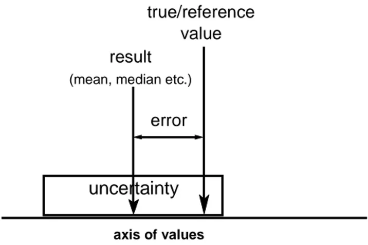
All measurements are affected by a series of nuisance effects that reduce the accuracy of the results thus introducing doubt into the values obtained. It is usually only pos-sible to give a range in which there is a certain probability of the true value being found.

Figure 1: Metrological concept of true value, uncertainty and error (Meinrath, 2000a)

The uncertainty associated with a measurement is an interval that cannot be corrected for. While the measured value is desired to be as close as possible to the true value, the uncertainty does not have an equivalent 'true' counterpart. There is nothing like 'true uncertainty'. Uncertainty is an instrument for communication between humans (commonly scientists) about the likely discrepancy between true and measured value. The importance of the communication tool 'uncertainty' must not be underestimated (Ellison, 1997). It is an essential tool in transferring information about the quality of knowledge obtained and the doubt to be reasonably associated with this knowledge. The complexity of our world and the activities taken place in it crucially depends on information with stated quality. Theoretical chemical speciation is only a minuscule element in this complexity. The decisions based in part on geochemical modelling for the performance assessment of nuclear waste repositories however have the potential to affect life on this world for some ten thousands of years.

Thermodynamic databases are often claimed to be consistent and as correct as possible. However, since stability constants generally are derived from experiment there will always be uncertainties in the determinations. The effect of these uncer-tainties on the speciation of an element in a given water may, in some cases, can be considerable (Ekberg, 1999). However, calculating such dependencies is very cumbersome to do by simple means even for a very simple case with only one ligand. Thus, for a more realistic case with several competing ligands, more elaborate methods are needed. There is also the problem of statistical sampling to make the obtained confidence interval good in a statistical sense. For these purposes the

L

LLJJJUUUNNNGGGSSSKKKIIILLLEEE program has been developed. It is an easy-to-use program with simple

menus in a WINDOWS environment.

uncertainty

result

(mean, median etc.)

axis of values

true/reference value

(12)

TheLL_LJJJUUUNNNGGGSSSKKKIIILLLEEE Code: Motivations

The abundance of fast computing power has largely simplified theoretical simulations of chemical equilibria even in rather complex solutions. A solubility is quickly calculated and a species diagram can be produced within a few minutes. Even those not well acquainted with computer programming languages may use freeware or commercial codes to produce such graphs. These graphs are, however, almost inevi-tably based in the mean values of certain thermodynamic quantities. It is not uncommon to find experimental observations interpreted within a tenth of a promille of a species read from a species distribution - based on uncertainty affected formation constants with up to a logarithmic unit of uncertainty (Ekberg, 2002).

In part, very far reaching conclusions are based on such theoretical simulations mostly without accounting for the uncertainties involved into such calculations. It has been shown elsewhere that existing thermodynamic data and data bases are neither consistent nor comparable. There is, however, no simple remedy in sight for this problem (Meinrath, 2002). The fundamental thermodynamic theory is available but our techniques are not yet powerful enough to warrant highest accuracy. If many uncertain parameters enter a calculation, the uncertainties accumulate and the calculation result will become comparatively vague. Uncertainty means doubt: the result of the calculation cannot be trusted arbitrarily. It is of outmost importance to evaluate a measure of the doubt involved. Despite this necessity, suitable tools for speciation calculations are not yet commonly applied.

A computer tool seemed appropriate that visualises the effect of the figures behind a '±' symbol on the result of a speciation calculation. There are good reasons to base such a tool on Parkhurst's PHREEQC code (Parkhurst, 1995) because PHREEQC is widely used, comparatively easy to learn, freeware, well maintained, versatile with a good manual, stable in execution and manageable in size and use of computer memory.

The LL_LJJJUUUNNNGGGSSSKKKIIILLLEEE code allows the user to select two approaches: the Monte Carlo

(MC) approach and the Latin Hypercube Sampling (LHS) (McKay 1979). Latin Hypercube sampling (LHS) allows to produce a satisfactory statistics with a minimum of CPU time. It is, in general, possible to do a simple theoretical speciation calculation within seconds. There are, admittedly, alternatives to LHS and there is criticism towards the uncritical use of LHS output because commonly correlation between some of the input variables exists. LHS, like MC, is not capable to take these correlations into account. Such a correlation can, i.e. exist between the pH of a solution and the partial pressure of CO2: higher pH solutions may absorb larger

amounts of CO2 and can reduce the CO2 partial pressure. It is therefore of advantage

to combine the both variables in a way that adequate pH/CO2 partial pressure pairs are

matched in the input vectors while LHS does not account for such correlations. Taken the generally rather poor degree of consistency, comparability and completeness in the existent thermodynamic data, however, such argumentation -justified as it is from a fundamental point of view- seems to be premature. It should be mentioned, however, that viable ways to account for correlation in input parameters have been reported in literature (Ekberg 1999 and references herein).

(13)

PROGRAM DESCRIPTION TheLL_LJJJUUUNNNGGGSSSKKKIIILLLEEECode

The LL_LJJJUUUNNNGGGSSSKKKIIILLLEEE program is written in the programming language C++ using the

Borland C++ builder (Borland). The program is divided into two major parts. One part containing the chemical calculations and one containing the statistical methods used. The basic idea is to make many runs with PHREEQC and in each run the stability constants of interest are changed slightly within their respective confidence interval according to the statistical method used (see below). Then, after each such cycle, if this option was selected, one of the factors may be changed by given increments to a given level, e.g. changing pH, and thus create a speciation diagram versus pH with uncertainty bands for each species concentration.

Chemical Calculations

The basic approach of the LL_LJJJUUUNNNGGGSSSKKKIIILLLEEE program is to use different statistical sampling

techniques to determine the effect of uncertain stability constants on a speciation calculation. The chemical speciation calculations are made by the well-known thermodynamic equilibrium program, PHREEQC. The chemical choices the user has to make are given in Figure 2: selecting species and formation constants (as a project file *.prj) whose formation constants will be varied and a database (*.dat) holding information on thermodynamic properties of other species.

(14)

Selection of project file: The project file holds all relevant information of the task to

be treated by LL_LJJJUUUNNNGGGSSSKKKIIILLLEEE code. If the project parameters are set, the water is defined,

the sampling method selected and the multiple run feature chosen or ignored, then Ljungskile is put to work by clicking "Simulation" in the menu. Before the code starts, the project file will have to be saved under a file name given by the user. If a project file is created from scratch, no name exists and a window will pop up ("Cannot create file"). The project file must be saved under a suitable name using "save as" in the File menu.

Selection of water: The user gives the chemical composition of a water together with

other quantities such as pH, pe and temperature. This information is then written in the input file to PHREEQC. Its filename is set by default to "PHREEQEC.IN" and cannot be changed. It is noteworthy that if the water is not charge balanced on input it will become so by the addition of an inert positive or inert negative element, Ip and Im, respectively. The concept of these species is briefly explained in Appendix III. Selection of database: The so-called thermodynamic databases are actually collections

of some mean values for formation constants and solubility products of a certain number of chemical compounds. The format is depending on the very program designed to read this data file. We will nevertheless stick with the common term 'database' in this manual. The choice of a certain database may influence the calculated result considerably. Hence, the user may generate his own database. As long as the database is in agreement with the PHREEQC format, the LL_LJJJUUUNNNGGGSSSKKKIIILLLEEE

output will be based on the selected database. In some cases the desired species are not present in the general database and therefore there is a possibility to change the database used. Note, that the species Im and Ip must be included into any self-created database in the way they are given in the example database.

Selection of sampling method: The sampling methods offered are the Monte Carlo

design and the Latin Hypercube design. The Latin Hypercube design is more efficient if a larger number of thermodynamic constants have been selected to vary in the project, while MC sampling is appropriate for just a handful of thermodynamic constants to vary. However, it is always helpful to have the possibility to compare different approaches and, hence, the MC approach is provided as a choice.

Selection of multiple run parameters: Sometimes it is also interesting to investigate

the evolution of a situation as a function of a parameter. The parameter, its starting and stopping value and the step width can be specified here. Note, that the multiple step feature has to be used wisely. Especially if solid phase dissolution and/or precipitation occur, the solution variations may become considerable. The

L

LLJJJUUUNNNGGGSSSKKKIIILLLEEE program accounts for charge balancing by adding 'virtual' species Im and

Ip but the result do not necessarily have to be meaningful. PHREEQC settings

As described above the water composition is given by the user together with pH, pe and temperature. If the given water composition results in an charge imbalance this is taken care of by the LL_LJJJUUUNNNGGGSSSKKKIIILLLEEE program. The method used is to use the inert

elements Ip and Im which are positive and negatively charged, respectively. This is made by first adding 1.10-6 M of Ip and then use the flag CHARGE. In case PHREEQC does not converge Im is used in the same manner and thus charge balance

(15)

is obtained. Thus it is simple to change the concentration of one of the elements present in the water without affecting the other water properties. This is a necessity since in a speciation diagram there is generally, at least, one factor changing along the x-axes.

Other settings in the PHREEQC input file is the use of the PRINT keyword. The flags used here are: -reset false, -totals true, -species. This is to make the result file clearer and more structured (interested readers are directed to the PHREEQC manual).

Some Comments on Statistical and Programming Methods

Statistics is looking for objective criteria to extract information from larger amounts of data. Data may be considered to be raw information in a qualitative or quantitative way. Data producers have the obligation to present all pertinent information that would impact on the use of it, to the extent possible. Of course, every possible use of data cannot be envisioned when it is produced, but the details of its production, its limitations and quantitative estimates of its reliability always can be presented. In an ideal situation, a reasonable measure of the doubt to be associated with given data will always be available.

There remains the task to act on basis of doubtful information. Within a computer program, handling and even creating uncertainty seems a contradiction to the fore-most abilities of a computer being a deterministic machine for invariable execution of instructions (Knuth, 1981).

However, the computer is a very helpful tool - and its helpfulness is the larger as there is no other tool to perform the task - to handle doubt and uncertainty a) because it is a deterministic machine b) because it is fast and c) because suitable algorithms exist. The use of computers for theoretical speciation calculations started rather early with the computer programs of Lars Gunnar Sillén in Sweden (Sillén, 1962; Sillén, 1964). Several major achievements have been included into Sillén's HALTAFALL model-ling codes: application of suitable minimisation routines for linear equations, suitable input formats for chemical information and programming techniques to accommodate all code in the tiny storage area of the early computers. Compared to these early applications, modern desktop machines represent the computing power of several computer centres in Sillén's time. Since then, storage capacity, CPU clock rates and algorithms have improved dramatically. The elements, however, have to be brought to work.

The sampling in the LL_LJJJUUUNNNGGGSSSKKKIIILLLEEE program is made by either simple Monte Carlo (MC)

sampling or Latin Hypercube sampling (LHS) (McKay, 1979), as described in detail in APPENDIX II. The basic step for LHS is to make a cumulative distribution function (cdf) for the sample based on the mean value and the standard deviation given for the respective variable (Meinrath, 2000a). Here the user may select how precise this cdf itself should be by selecting how many points are to be included in its construction. The samples are then drawn from this empirical cdf, as described in APPENDIX II. For the MC sampling there is no extra work since this method samples complete randomly within the given interval/distribution. Random number generators are further discussed in APPENDIX I.

(16)

In the current version of the LL_LJJJUUUNNNGGGSSSKKKIIILLLEEE program there are two distributions and two

sampling methods to select from. The distributions are the uniform distribution and the normal distribution. The sampling intervals are given slightly different for the two distributions. The uniform distribution requires a highest and a lowest value while the normal distribution uses a mean and a standard deviation.

TheLLJJUUNNGGSSKKIILLEEDisplay Program

L

LDDP is intended to graphically display the results obtained by the P LL_LJJJUUUNNNGGGSSSKKKIIILLLEEE

'multiple run' option. It is not a sophisticated graphics program but kept comparatively simple. LLDDP gets its information mainly from the respective project file in the \results\P

directory. The LL_LJJJUUUNNNGGGSSSKKKIIILLLEEE program copies these files to the results directory and

renames the project file into an *.ldp file. Thus, LLDDPP is set by default to open an *.ldp file and searches its respective input files in the same directory. From the different output files LLDDPP can create a variety of diagrams. In fact, the diagram displayed may vary considerably depending on the task given to the LL_LJJJUUUNNNGGGSSSKKKIIILLLEEE program. In

general, the user can select three different ordinate presentations: the concentration, the logarithm of the concentration and the percentual distribution.

IfLL_LJJJUUUNNNGGGSSSKKKIIILLLEEE has calculated a multiple run problem, e.g. a speciation as a function of

pH, then the output is a speciation diagram as function of pH. The uncertainties are displayed as approximate 68% confidence percentiles. The code selects the calculated value closest to the 0.68 percentile. Hence, the 0.68 percentile is the closer approxi-mated the more LHS cycles are calculated.

The concentration presentations are calculated from the *.out files saved by the

L

LLJJJUUUNNNGGGSSSKKKIIILLLEEE program in the path\results\*.prj directory. Species distribution is

calcu-lated from the phrout.* files. The program recalculates the species distribution for each run from the concentration information, evaluates the empirical distribution function and chooses the value closest to the 0.16 percentile, the median and value closest to the 0.84 percentile value as uncertainty limits and centre, respectively. It is obvious that a small number of runs provides a more variable uncertainty value than a larger number of runs. It should be kept in mind that the LLjjuunnggsskkiillee code wants to visualise the uncertainties in sets of formation constants. For several reasons these visualisations can be approximations only. The experience with LLjjuunnggsskkiille calcula-e

tions show, however, the necessity of an attitude of great carefulness that should be taken towards speciation calculations.

The diagram has two further options: The user can choose the presentation of the abscissa in logarithmic format or linearly. A logarithmic presentation does not make sense if the abscissa variable is pH. The second option allows to display the location of the points calculated in the LL_LJJJUUUNNNGGGSSSKKKIIILLLEEE run in the shape of crosses. A displayed

data set can be saved as ASCII file to be converted to a presentation graphics by a suitable graphics program (e.g. ORIGIN).

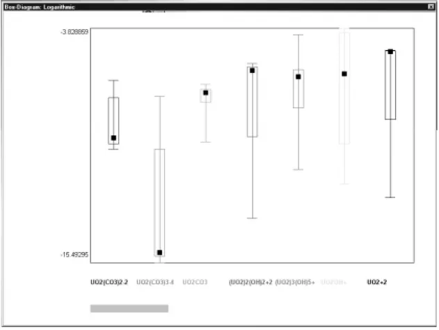
IfLL_LJJJUUUNNNGGGSSSKKKIIILLLEEE calculated a single run option, e.g. the distribution of metal ion species

at a given pH, then the results are displayed as simplified box plots. The box in the centre gives the median value while the usually wider open box indicates 0.68 percentiles. The bar line indicates the total range of the property. Note that for small number of runs it is not uncommon that some values coincide. Again the user may select different presentation types. The LDP code recognises from the *.ldp file whether the single run option has been chosen and the respective graphical

(17)

presenta-tion is displayed as shown in fig. 3. The box plot presentapresenta-tion can be saved. The five respective characteristics are saved as numerical values.

It should be mentioned that most presentation programs or statistical data evaluation programs do have a box plot option corresponding to Tukey's original definition of box plots. The user may prefer to import the data calculated from the LL_LJJJUUUNNNGGGSSSKKKIIILLLEEE

code into such a commercial program.

(18)

Installation and Description of Files

Installation: LL_LJJJUUUNNNGGGSSSKKKIIILLLEEE program and LLLJJJUUUNNNGGGSSSKKKIIILLLEEE Display Program (LLDDP)P

The LL_LJJJUUUNNNGGGSSSKKKIIILLLEEE files must be copied manually into a suitable directory. In the

following, it is assumed that the program files are copied to a directory D:\Ljungskile. A subdirectory \results has to be created before LL_LJJJUUUNNNGGGSSSKKKIIILLLEEE is executed the first time.

In the \results subdirectory, LL_LJJJUUUNNNGGGSSSKKKIIILLLEEE generates a subdirectory with the name of the

project file *.prj. Assuming a project file "Test.prj", the results calculated by

L

LLJJJUUUNNNGGGSSSKKKIIILLLEEE would be found in the directory D:\Ljungskile\results\Test.

TheLL_LJJJUUUNNNGGGSSSKKKIIILLLEEE Display Program is installed by an installation routine.

Description of Files: LL_LJJJUUUNNNGGGSSSKKKIIILLLEEE code

The files made by or needed for the LL_LJJJUUUNNNGGGSSSKKKIIILLLEEE programs are listed below.

PHREEQC.EXE The thermodynamic equilibrium program used for the chemical calculations.

LJUNGSKILE.EXE Master program which runs all screen handling and user interface. This program also manipulates the database and the input file to PHREEQC according to the selections of the user

SIMULATION.EXE Runs PHREEQC and checks its results

“project name”.PRJ Contains all information related to the selected project (created by the program).

PHROUT.# Contains raw data from each simulation cycle (#) (created by the program)

PHROUT.AVR Contains average concentrations of the selected species (created by the program)

PHROUT.SD Contains the estimated standard deviation of the selected species concentrations obtained by the setting selected for this calculation (created by the program)

The following file names are either generated or used by the programs temporarily and therefore the user must not add or delete any of them manually unless clearly aware of what one is doing.

(19)

PHREEQC.DAT (needed by the program) PHREEQC.OUT (created by the program) PHREEQE.IN (created by the program) PHREOUT.AVR (created by the program) PHROUT.SD (created by the program)

The database file “database”.dat must contain the inert elements Ip and Im as shown in APPENDIX III.

Description of Files: LL_LJJJUUUNNNGGGSSSKKKIIILLLEEEDisplay Program (LLDDP)P

After installing LLDDP, it starts by clicking the LDP.exe file in the installation directory.P

From the "File" menu, the "Open" feature has to be selected and a suitable

L

LLJJJUUUNNNGGGSSSKKKIIILLLEEE project file (*.prj) must be selected. LLDDPP reads the relevant information

from the project file and displays the 'multiple run' calculations accordingly.

Three different ordinate presentations can be selected from the "Diagram" menu: concentration, logarithmic concentration and relative distribution. In all cases, the mean values are given as solid lines while the upper and lower 0.68 percentile values are given as dashed lines. LDP uses 15 different colours to display the lines of diffe-rent species. If more than 15 species are included into the LL_LJJJUUUNNNGGGSSSKKKIIILLLEEE calculation,

then some colours will be used twice. Experience shows that diagrams with more than ten relevant species already get messy, anyway.

Graphical presentation

TheLLDDP graphical representation fits itself to the screen resolution. It is neverthelessP

possible to resize and to move the diagram. LLDDP does not create a grid to the diagram.P

Only minimum and maximum ordinate and abscissa values are given. But if the cursor moves over the diagram, its coordinates according to the diagram scale are given.

Diagram check boxes

The diagram offers two check boxes: "logarithmic abscissa" and "show data as crosses":

"Logarithmic abscissa": LL_LJJJUUUNNNGGGSSSKKKIIILLLEEE saves the abscissa values linearly. If LLLJJJUUUNNNGGGSSSKKKIIILLLEEE

's "logarithmic scale" feature is selected in the 'multiple runs' window, the value is not saved as, say, -5.5 but as 3.162278E-6. An exception is pH. Hence, checking and unchecking the box will allow to switch between the linear and the logarithmic scale. "show data as crosses": LL_LJJJUUUNNNGGGSSSKKKIIILLLEEE calculates values at fixed intervals. In generating

the diagram, LLDDPP interpolates linearly between the calculated values. By checking the box, the density of calculated points can be visualised.

(20)

Exporting diagram data

There is no "print" feature in LLDDPP. Instead, the graphical data can be exported in ASCII format by selecting "save" from the "File" menu. The data is saved with the default extension *.psa. For each abscissa value, respective ordinate values are stored in a chain consisting of the sequence "upper, lower and median value" of each species. To allow identification, the date of the generated file is added as the final datum. The *.psa file can be imported into a suitable scientific presentation program and manipulated according to the needs of the user.

File information

To allow a quick overview on some basic data from the project file, the menu feature "Information" displays a brief list.

(21)

Getting Familiar: A Step-by-Step Example

Once the LL_LJJJUUUNNNGGGSSSKKKIIILLLEEE code is installed, the directory where the code is installed

should include the files (in the following "d:\Ljungskile\" is assumed). Ljungskile.exe

Simulation.exe Phreeqc.exe example.prj example.dat

The file example.dat holds a thermodynamic data base. This data base is part of the PHREEQC package (Parkhurst 1995) and further information can be found in the PHREEQC manual (download under http://water.usgs.gov/software/phreeqc.html). Advantageously the PHREEQC database can be extended and modified with comparative ease. The user is encouraged to display this database in a text processor program like Wordperfect, Word or StarWriter and study how to modify it.

(22)

In order to run, the LL_LJJJUUUNNNGGGSSSKKKIIILLLEEE code needs information: first on the data base (several

data bases may be provided by the user) and second on the specific tasks summarised in a project file. Clicking on the project file example.prj will highlight it together with the Latin Hypercube feature in the field 'sampling method'. Clicking on "example.dat" in the right side selection box will make the project window "example.prj" available for user editing. The user is advised to examine the editing and selection windows but is recommended not to make any changes at this level of the example.

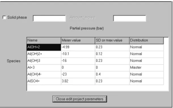
Figure 5: Speciation window of LL_LJJJUUUNNNGGGSSSKKKIIILLLEEE. The user can change the

thermodynamic parameters, the uncertainties and the distribution for each species. Species can be added and deleted. The respective window pops up on clicking the right mouse button. The species name must be present in the database (case sensitive).

The first column of the project window table gives the species names. These names have to be in agreement with the PHREEQC data base conventions (see PHREEQC manual) and to be present in the selected database. A species Al(OH)4- can appear in

the database as "AlOH4-", "Al(OH)4-" or even "O4H4Al-". The form given in the table must correspond to whatever form the database holds. In a similar way the formation constants have to comply with the PHREEQC sign conventions.

Depending on the uncertainty distribution of choice, the standard deviation (normal distribution) or a maximum value (uniform distribution) have to be specified. The distribution itself is specified in the last column.

It is possible to select a solid as solubility limiting phase in order to calculate mineral solubilities. The name of the solid phase must correspond to a mineral name in the selected database. In the amount field a value can be entered (in units of mol L-1). If no value is specified, the amount is assumed to be zero and only precipitation processes can be calculated. Otherwise, the amount specified may be dissolved and change the water composition. Solid phases often change the physicochemical proper-ties drastically. To warrant convergence in PHREEQC, the composition of the water should be close to the final composition. This can be achieved by calculating a single

(23)

step run, checking the composition of the final solution in the PHREEQC.OUT file and modifying the water composition accordingly. The 'virtual' species Ip and Im will warrant charge balance otherwise. These reactions may alter the solutions conside-rably causing non-convergence.

Species can be added or deleted upon clicking the right mouse button and making the appropriate selection from the pop-up window. An added species must occur in the database and typed correctly (case sensitive). The button 'close edit project para-meters' will close the project window.

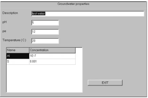
An interesting feature of any speciation program is the calculation of equilibria in complex solutions. Laboratory solutions usually strive for a simple composition - the simple composition in turn allows a theoretical speciation without complex computational tools like the LL_LJJJUUUNNNGGGSSSKKKIIILLLEEE code. However, the situation in

ground-waters is usually less straightforward. The 'edit water' button in the 'project' frame allows to specify pH, pe, temperature and total concentrations of water components to be considered in the LL_LJJJUUUNNNGGGSSSKKKIIILLLEEE speciation. The elemental composition can be

modi-fied by adding or deleting elements. Elements are added by clicking the right mouse button. Leave the water unchanged for running the example project.

Figure 6: Water window of LL_LJJJUUUNNNGGGSSSKKKIIILLLEEE. The description should be chosen to allow

clear identification of the file. The pH can be specified but it will be overridden if pH is chosen later as running variable in the 'Multiple run' window (see below).

The last window is the 'Method' window (Fig.7) where the upper left hand side box allows us to choose between a Monte Carlo method and the Latin Hypercube approach. For the present case, we will stick with the Latin Hypercube method. The

(24)

specifies the number of normally and uniformly, respectively, distributed random points used by the program in constructing a cumulative normal distribution. It is reasonable to have the '#runs' value smaller than the '#points in the cdf'. Otherwise the program issues a warning otherwise but it can be overridden.

Figure 7: Method window of LL_LJJJUUUNNNGGGSSSKKKIIILLLEEE. Method for probabilistic calculation

(Monte Carlo or Latin Hypercube Sampling), the starting value of the random number generator and some details of the cumulative distribution functions (cdf's) can be selected.

This example will follow the speciation over a certain pH range. Such a calculation will nicely illustrate what the LL_LJJJUUUNNNGGGSSSKKKIIILLLEEE code can be used for. On checking the 'use

multiple runs' box, the following window should open:

Figure 8: Multiple Runs window of LL_LJJJUUUNNNGGGSSSKKKIIILLLEEE.

The running variable can be selected from the left hand side drop-down field. The start and end values of the running variable must be specified together with an interval length. The selection field "Logarithmic scale" will be active by default as soon as a parameter other than pH or pe is selected. The user can set it inactive if he desires it for some reason. However, it would be unreasonable to vary, say, the Al total

(25)

concen-tration between 10-7 M and 10-3 M in steps of 10-6 M - ending up in several thousand steps. A typical situation for inactivating this feature is the selection of temperature as variable.

In the left hand side selection box, the variable parameters are listed. The pH should be selected. The meaning of 'Start', 'Stop' and 'Interval length' explain themselves and should be filled with the values '3', '7' and '0.1'.

Now, the procedure can be started by clicking on the 'Simulation' menu item. PHREEQC runs in a DOS box. It is possible to run the calculations in the background and to use the computer for other purposes at the same time. The simulation takes some minutes to complete. The progress bar indicates the degree of completion.

Description of Output

After completion of the calculations a new subdirectory in the LL_LJJJUUUNNNGGGSSSKKKIIILLLEEE

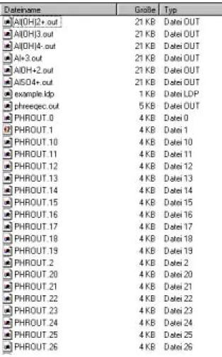
installation directory has been created: \results. The project name specifies a subdirectory in \results. Hence, in the present example, the calculated information is found in D:\Ljungskile\results\example\. The top section of this subdirectory is shown in Fig. 9.

(26)

There are 41 Phrout.xx (xx = 1 to 41) files, one Phrout.avr and one Phrout.sd file. For each of the six species X.out files are available (X = Al(OH)4-, Al+3, AlSO4+, Al(OH)2+, Al(OH)3, AlOH+2). These files can be inspected with a word processor and it is recommended to do so for illustrative purposes.

In the present situation, the files Phrout.avr and Phrout.sd are of major interest because they hold the mean values (Phrout.avr) and the standard deviations (Phrout.sd) of the calculated species concentrations:

The Phrout.avr file for the Al speciation example

pH 3.00000e+00 3.10000e+00 3.20000e+00 3.30000e+00 3.40000e+00 3.50000e+00 3.60000e+00 3.70000e+00 3.80000e+00 3.90000e+00 4.00000e+00 4.10000e+00 4.20000e+00 4.30000e+00 4.40000e+00 4.50000e+00 4.60000e+00 4.70000e+00 4.80000e+00 4.90000e+00 5.00000e+00 5.10000e+00 5.20000e+00 5.30000e+00 5.40000e+00 5.50000e+00 5.60000e+00 5.70000e+00 5.80000e+00 5.90000e+00 6.00000e+00 6.10000e+00 6.20000e+00 6.30000e+00 6.40000e+00 6.50000e+00 6.60000e+00 6.70000e+00 6.80000e+00 6.90000e+00 7.00000e+00

AlOH+2 1.37451e-09 1.55039e-09 1.75745e-09 1.99996e-09 2.28252e-09 2.60777e-09 2.97640e-09 3.38607e-09 3.83251e-09 4.30682e-09 4.79862e-09 5.29357e-09 5.77717e-09 6.23552e-09 6.65509e-09 7.02376e-6.65509e-09 7.33232e-6.65509e-09 7.57352e-6.65509e-09 7.74210e-6.65509e-09 7.83411e-6.65509e-09 7.84555e-6.65509e-09 7.77333e-6.65509e-09 7.61357e-09 7.36324e-09 7.02051e-09 6.58635e-09 6.06730e-09 5.47719e-09 4.83857e-09 4.18147e-09 3.53948e-4.18147e-09 2.94454e-4.18147e-09 2.41993e-4.18147e-09 1.97790e-4.18147e-09 1.61884e-4.18147e-09 1.33368e-4.18147e-09 1.10761e-4.18147e-09 9.23557e-10 7.65781e-10 6.22782e-10 4.89240e-10

Al(OH)2+ 6.81271e-13 1.09048e-12 1.73253e-12 2.73038e-12 4.26559e-12 6.60065e-12 1.01082e-11 1.53089e-11 2.29050e-11 3.38504e-11 4.93769e-11 7.10836e-11 1.00985e-10 1.41683e-10 1.96382e-10 2.68909e-1.96382e-10 3.63663e-1.96382e-10 4.85250e-1.96382e-10 6.37578e-1.96382e-10 8.22895e-1.96382e-10 1.04086e-09 1.28900e-09 1.56331e-09 1.85882e-09 2.16903e-09 2.48293e-09 2.78453e-09 3.05224e-09 3.26141e-09 3.38853e-09 3.41744e-3.38853e-09 3.34310e-3.38853e-09 3.17329e-3.38853e-09 2.92613e-3.38853e-09 2.62620e-3.38853e-09 2.29953e-3.38853e-09 1.96929e-3.38853e-09 1.65369e-09 1.36470e-09 1.10882e-09 8.88210e-10

Al(OH)3 5.98660e-16 1.21069e-15 2.42869e-15 4.83085e-15 9.51976e-15 1.85708e-14 3.58336e-14 6.83294e-14 1.28670e-13 2.39092e-13 4.38178e-13 7.91818e-13 1.41083e-12 2.47971e-12 4.30151e-12 7.36521e-4.30151e-12 1.24501e-11 2.07690e-11 3.4164.30151e-12e-11 5.53159e-11 8.80574e-11 1.37667e-10

The .avr and .sd files provided by LDP can be used for getting a quick survey on the results using a short program in the style given in Appendix IV. The generated ASCII files may subsequently be imported into a presentation graphic program like SigmaPlot or ORIGIN.

(27)

TheLL_LJJJUUUNNNGGGSSSKKKIIILLLEEE Display Program (LDP)

A convenient way to display the output of a LL_LJJJUUUNNNGGGSSSKKKIIILLLEEE run is provided by a

supplement, the LL_LJJJUUUNNNGGGSSSKKKIIILLLEEEDisplay Program (LLDDP). If LDP has been installed inP

the same directory as the Ljungskile.exe, LLDDP can be started from the P LL_LJJJUUUNNNGGGSSSKKKIIILLLEEE

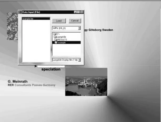
screen by clicking the 'Display' menu item. Start LLDDP and select the example.ldp fileP

in the subdirectory \results\example by selecting 'Open' from the file menu.

Figure 10: select 'example.ldp' from the respective \results\ subdirectory

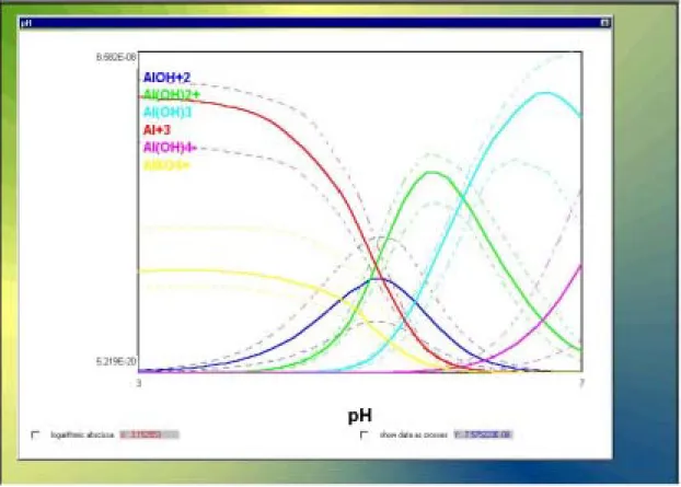
Figure 10 shows the resulting screen. In the diagram constructed by LLDDP (Fig. 11) theP

names of the species are listed and the colour of the species name corresponds to the respective colour of the calculated curve. The upper and lower .68 percentiles are shown as dashed lines. The diagram may be resized and moved around.

The x and y coordinates under the cursor are numerically given in two fields below the diagram. Click on the respective field to make LLDDP show the actually measuredP

points.

Select 'distribution' from the 'Diagram' menu and see the changes. Select 'Save' from the file menu and save the data as ASCII files under the extension *.psa for postprocessing by a graphics program.

(28)

Figure 11: Species concentrations as a function of pH calculated for example.prj

conditions.

Figure 12: The 'example' results in an ORIGIN presentation format

3 4 5 6 7 0 25 50 75 100 total Al3+ : 1.10-7 mol L-1 AlSO+₄ Al(OH)-₄ Al3+ Al(OH)°₃ Al(OH)+₂ AlOH2+ re la ti v e a m oun t / [% ] pH

(29)

References

http:\\www.borland.de

Box G.E.P, Muller M.E. (1958) A Note on the Generation of Random Normal Deviates. Ann. Math. Stat 29: 610 - 611

Ekberg C., Emrén A.T. (1993) Finding and Correcting Calculation Errors in PHREEQE. Proc. Int. Conf. Migration 93 Charleston/USA. Oldenbourg Verlag München/FRG.

Ekberg C. (1999) Uncertainty in Actinide Solubility Calculations Illustrated Using the Th-OH-PO4 System. Thesis. Chalmers University of Technology.

Ekberg C., Emrén A.T. (2001) Uncertainties in Solubility Calculations. Monatshefte Chemie 132: 1171

Ekberg C. (2002) Uncertainties Connected with Geochemical Modelling of Waste Disposal in Mines. Mine Water Environ 21: 45 - 51

Ellison S., Wegscheider W. and Williams A. (1997) Measurement Uncertainty. Anal Chem 69: 607A - 613A

Knuth D.E. (1981) The Art of Computer Programming 2nd ed.. Vol II: Seminume-rical Algorithms. Addisson-Wessley, Reading/USA

McKay M.D., Conover W.J., Beckman R.J. (1979) A Comparison of Three Methods for Selecting Values of Input Variables in the Analysis of Output of a Computer Code. Technometrics 21: 239 - 245

Meinrath G., Ekberg C., Landgren A., Liljenzin JO (2000) Assessment of Uncertainty in Parameter Evaluation and Prediction. Talanta 51: 231 - 246

Meinrath G (2000a) Comparability of Thermodynamic Data - A Metrological Point of View. Fresenius J Anal Chem 368: 574 - 584

Meinrath G, Hurst S, Gatzweiler R (2000b) Aggravation of Licensing Procedures by Doubtful Thermodynamic Data. Fresenius J Anal Chem 368: 561 - 566

Meinrath G (2001) Measurement Uncertainty of Thermodynamic Data. Fresenius J Anal Chem 369: 690 - 697

Meinrath G, May PM (2002) Thermodynamic Prediction in the Mine Water Environment. Mine Water Environ. 21: 24 - 35

Parkhurst D.L. (1995) Users Guide to PHREEQC - A Computer Program for Speciation, Reaction-Path, Advective-Transport, and Inverse Geochemical Calculations. Water-Resources Investigations Report 95-4227. U.S. Geological Survey Lakewood, Colorado/USA.

(30)

Sillén L.G. (1962) Acta Chem Scand 16: 159

Sillén L.G. (1964) High-Speed Computers as a Supplement to Graphical Methods. III. Twist-Matrix Methods for Minimizing the Error-square Sum in Problems with Many Unknown Constants. Acta Chem Scand 18: 1085 - 1098

Wolery T.J. (1992) EQ3/6, A Software Package for Geochemical Modeling of Aqueous Solutions: Package Overview and Installation Guide (Version 7.0). REPORT UCRL-MA-110662 PT 1, LLNL, Livermore CA/USA

(31)

APPENDIX I

Random Numbers

Computer-generated random numbers are not truly random because they result from deterministic process. Theoretically and despite the seemingly perfect randomness of generated random numbers, the deterministic law behind a computer-generated sequence of 'random numbers' can be resolved provided enough resources will be invested. However, by combining two random processes such efforts will be in vain even for very long sequences of random numbers and thus the differences between truly random processes and computer-simulated random processes becomes academic. The following procedures describe the random number generators used in the present implementation of LL_LJJJUUUNNNGGGSSSKKKIIILLLEEE code. The algorithms are well known in

literature on algorithms and are mostly summarised by Knuth (1981). Additional sources will be occasionally given below in order to direct the reader to further information of interest.

Linear random number generator

A linear random generator returns a number from a specified range (commonly 0 and 1) where one number is equally likely to occur. The linear random number generator thus returns uniform random deviates (to be distinguished from the normally distributed random deviates discussed later). The algorithm of a linear random generator calculates an integer number Ik+1from a previous number Ik by

Ik+1 = a Ik + b (mod c) (1)

where I gives a random number, k the running index, a the multipliers, b the increment and c the modulus. The numbers a, b, and c are positive integer numbers. The modulus c gives the length of the chain after which the process (1) repeats itself. Therefore, the larger c the longer the chain. A random number between 0 and 1 is obtained by dividing Ik+1/c. The recurrence formula (1) requires a starting value, also

termed 'seed'. The seed is allowed to be user-specified in LL_LJJJUUUNNNGGGSSSKKKIIILLLEEE code.

Since the random number generator of type (1) may have many deficiencies (i.e. serial correlation and bad selection of the value for a, b and c), additional shuffling is done: the random number generator is used to fill an array of, say, 100 figures with random numbers. After this preparation, a random number is chosen based on a first random number generated (converted into an index of the array) and is replaced by a second random number. By coupling two suspicious processes of 'insufficient randomness', an almost perfect random number can be generated.

Normally distributed random deviates

Normally distributed random deviates with a mean of 0 and a standard deviation of 1 can be efficiently obtained by an algorithm of Box and Muller (1958) from a linear random generator.

(32)

On basis of two values LRG1 and LRG2 v1 = 2 * LRG1 - 1

v2 = 2 * LRG2 - 1

and the acceptance condition q = v12 + v22

0 < q < 1

the normal deviates NRD are calculated by

NRD1 = f . v1

NRD2 = f . v2

A cumulative normal distribution can be approximated by generating a larger series of N normally distributed random deviates, sorting them with increasing magnitude and putting a weight of 1/N on each value. Intermediate values of the thus generated cumulative normal distribution can be obtained by interpolation (Meinrath, Ekberg et al., 2000).

There are, admittedly, alternative and probably computationally more efficient ways in obtaining a normally distributed random deviate with defined uncertainty by using Chebyshev approximations of a scaled cumulative Gaussian distribution. In the pre-sent case, however, the computational burden imposed by the method selected for implementation in the LL_LJJJUUUNNNGGGSSSKKKIIILLLEEE code is almost irrelevant compared to the CPU

time required for the PHREEQC speciation calculations that further optimisations seem irrelevant under the overall aspect.

q ) q ln( 2 f = − ⋅

(33)

APPENDIX II

Latin Hypercube Sampling

Computer models are in common instruments for simulation of complex models in many areas of industry and science. Models allow to investigate intricate relationships on a broad level. Models summarise information obtained from data and may forward knowledge of highest complexity. Since each input variable is affected by uncertainty, the predictive power of a computer model is influenced by the evolvement of these uncertainties during a simulation run.

It is always possible to choose a Monte Carlo design for a study of the influence of input variable uncertainties on simulation output. There are, however, many input variables in even a simple theoretical speciation calculation and the Monte Carlo study consequently must involve a large number of runs. It must be ensured that for each input variable the probability distribution is sufficiently represented in the Monte Carlo runs. This representation is almost warranted for input values close to the mean value. But with larger distance from the mean value, inclusion becomes less and less likely. Consequently, the more uncertain input variables are to be considered, the larger the number of Monte Carlo runs has to be.

There is no need to delve into the question how to estimate the necessary number of runs conditional on the number of input variables. There are more efficient strategies. An especially clever and simple strategy has been suggested by McKay, Conover and Beckman (1979).

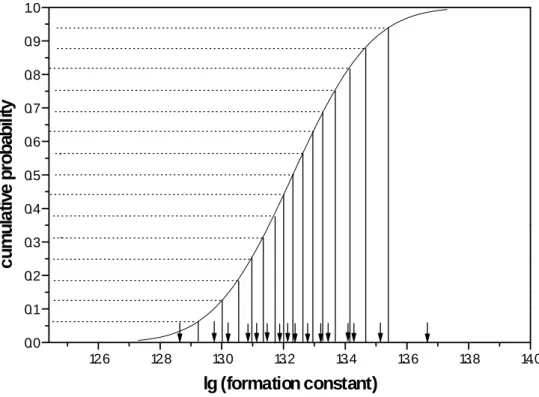
Figure A1: A cumulative normal distribution stratified into 16 strata of equal

probability. The bottom arrows indicate the randomly drawn representatives for each

12.6 12.8 13.0 13.2 13.4 13.6 13.8 14.0 0.0 0.1 0.2 0.3 0.4 0.5 0.6 0.7 0.8 0.9 1.0 c u m u la ti v e pr oba bi lit y lg (formation constant)

(34)

Latin Hypercube Sampling (LHS) requires a division of the cumulative probability distribution of each of n input variables to be divided into n bins of equal probability 1/n. Such a case is shown in Fig.1 for a cumulative normal distribution of mean 13.23 and ±.68 percentiles of 0.2. The distribution is divided into 16 sections of equal probability 1/16. The bottom arrows indicate a randomly chosen value from within the interval to represent the interval in the LHS procedure. In generating the intervals of equal probability, an arbitrary choice has to be made with respect to the position of the lower and upper boundary that is set in the present example to four times a .68 percentile. The probability of an event with a value larger than 14.03 is below 0.00001 and can safely be neglected in a LHS design on basis of 16 events. For very large designs it may be considered to set the lower/upper limit to ±4 .68 percentiles but the likely variation most probably will be almost probably negligible.

In an LHS design, the number of strata is given by the total number of uncertainty affected input variables to be included into a simulation run. Thus, for each of the n input variables n values are selected that represent all parts of a distribution with the adequate probability. Hence, the risk to either ever-present or underrepresented certain sections of a distribution is greatly reduced.

From the n × n input variable (representatives of n strata for n variables), input vectors into the computer simulation have to be constructed. An obvious choice is to randomly chose one representative for each variable, to run the simulation and the repeat the random selection until all representatives have been exhausted in n simulations. But even so an obvious option, random sampling is not optimal.

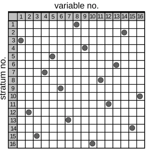
There is a more clever way to construct input vectors. This method is shown in fig. A2. Please note that in each row only one representative is to be found. It is not possible, for example, to have several representatives of the stratum 3 in one input vector while other strata are not considered in a certain input vector. Such a vector may occur in random sampling but not in Latin Hypercube Sampling. It is necessary to generate the remaining 15 input vectors in accordance with the same construction principle.

Form the n runs, n realisations of the simulation output are obtained, from which mean values and standard deviations may be estimated according to the well known statistical formula on basis of a normal distribution assumption. In case of larger samples, an alternative is to generate the empirical probability densities and to evaluate median and upper and lower percentiles (Meinrath, Ekberg et al. 2000). The

L

(35)

Figure A2: Example of one of 16 input vectors created from 16 strata of 16 input

variables according to the LHS strategy.

1 2 3 4 5 6 7 8 9 10 11 12 13 14 15 16

1

2

3

4

5

6

7

8

9

10

11

12

13

14

15

16 variable no.

stratum no.

(36)

APPENDIX III

The Virtual Species Im and Ip

In many cases in geochemical modelling it may be desired to keep the water parameters pH and pe constant during a calculation. One such example is the solubility of some mineral at a given pH and pe. Without precautions, dissolution and/or precipitation may change the solution composition that drastically, that a fixed value for pH and/or pe cannot be reached by the PHREEQC code. The solution parameters may change due to the dissolution or the precipitation and thus the solution obtained is not any longer similar to the starting solution.

PHREEQC is designed to solve a precipitation/dissolution reaction and to print out composition of the equilibrium solution. Thus PHREEQC is capable of describing the process of putting a piece of mineral in a certain water and then calculate what has happened. But in the LL_LJJJUUUNNNGGGSSSKKKIIILLLEEE program's "multiple run" feature, the goal is a

different one. We would like to know what the solubility would be in a water at a given pH and pe. To facilitate this the inert elements Ip (inert positive) and Im (inert negative) have been introduced into the PHREEQC database. Im and Ip enter the calculation of ionic strength, but do not react, e.g. by forming complexes. The entry in the PHREEQC database is shown below:

a) add in the database head:

and in the species definition section:

It should be noted that the numbers assigned here does not have to be the ones used in any given situation. With this modification it is possible with the aid of the keyword CHARGE to fulfil the charge balance condition, and thus keeping the pH or pe constant during dissolution or precipitation by addition of either Ip or Im. The same features could, naturally have been accomplished by addition of some other element but then the complexing behaviour of the solution would have changed.

The case of redox instabilities it has been described elsewhere (Ekberg 1993) for the older FORTRAN PHREEQE but the adoption to PHREEQC format is straight forward.

(37)

APPENDIX IV

A Rough and Dirty Way to Use LL_LJJJUUUNNNGGGSSSKKKIIILLLEEE Output

The Ljungskile output can also be used without the Ljungskile Display Program. For that purpose, its needs to be extracted from the respective output files. An example is given in the following. The user has to specify the necessary information, e.g. the number of steps and the number of LHS samples used in the calculations. Depending on the program used to cast the numerical information into a graphical form, some rearrangement of the data may be necessary. The final graphical result is shown in fig. A3.

Figure A3: Distribution of Al(III) species in an aqueous solution of low

mineralisation as a function of pH. Solid lines give mean concentrations while the dashed lines gives 1σ upper and lower standard deviations. Note the negative concentrations for the Al(OH)2+ species. LDP is using the empirical distributions and

will not result in negative concentrations.

It is also possible to calculate the information given in files Phrout.avr and Phrout.sd directly from the results in each of the files X.out. Depending on the post processing purpose this way may be even more convenient (the computer does the number crunching e.g. via a short QBasic program).

The code below opens the file X.out (the species specific part is given by the variable d$), evaluates the mean and the standard deviation and writes the lower boundary (mean-sd), the mean and the upper boundary (mean+sd) to a X.dat file. Please note that the names of the PHREEQC output files cannot be read directly by QBasic and the non-ANSI characters (generally '+' characters in file names) must be eliminated.

3 4 5 6 7 0 2x10-8 4x10-8 6x10-8 8x10-8 1x10-7 AlSO+₄ Al(OH)-₄ Al(OH)°₃ Al(OH)+₂ AlOH2+ Al3+

[c

o

n

c

e

n

tr

a

tio

n

]

pH

(38)

Note that the upper and lower confidence limits are symmetric with respect to the mean value curves. This behaviour is caused by the simplified calculation in the Qbasic code based on the assumption of identically and independently distributed residuals with zero mean. The calculation of the calculated data however shows that in most cases the distributions are skewed. In the simplified form it may even be observed that lower uncertainties are below zero. LDP analyses the distributions and evaluates approximations to the .68 percentiles about the median. These percentiles take skewness into account and present asymmetric upper and lower confidence bands.

'************ Ljungskile Evaluation **************************************** SCREEN 12

CLS

d$ = "alSO4": REM "Al3", "AlOH2", "Al(OH)2+", "Al(OH)3", "Al(OH)4" dname$ = "d:\eigene~1\" + d$ + ".out"

dout$ = "d:\eigene~1\" + d$ + ".dat" OPEN dname$ FOR INPUT AS #1

OPEN dout$ FOR OUTPUT AS #2

test$ = "element species": REM input of text headers in the .out files WHILE a$ <> test$ LINE INPUT #1, a$ WEND LINE INPUT #1, a$ i = 0 a = 0 INPUT #1, pH WHILE NOT EOF(1)

b = a INPUT #1, a IF a < 3 OR a > 7 THEN i = i + 1 sum1 = sum1 + a sum2 = sum2 + a * a ELSE IF a >= 3 AND a <= 7 THEN sum1 = sum1 - b sum2 = sum2 - (b * b) i = i - 1 sum1 = sum1 / i sum2 = sum2 / i

sd = SQR(ABS(sum2 - (sum1 * sum1))) WRITE #2, pH, sum1, sum1 - sd, sum1 + sd

i = 0 pH = a sum1 = 0 sum2 = 0 sd = 0 END IF END IF WEND sum1 = sum1 - b sum2 = sum2 - (b * b) i = i - 1 sum1 = sum1 / i sum2 = sum2 / i

sd = SQR(ABS(sum2 - (sum1 * sum1))) WRITE #2, pH, sum1, sum1 - sd, sum1 + sd CLOSE #1

CLOSE #2 END

2003:03 LJUNGSKILE 1.0

SKI Report 2003:03

Research

LJUNGSKILE 1.0

A Computer Program for Investigation of

Uncertainties in Chemical Speciation

Christian Ekberg

Arvid Ödegaard-Jensen

Günter Meinrath

SKI perspective

SKI Report 2003:03

Research

LJUNGSKILE 1.0

A Computer Program for Investigation of

Uncertainties in Chemical Speciation

Christian Ekberg¹

Arvid Ödegaard-Jensen¹

Günter Meinrath²

³

¹Department of Nuclear Chemistry

Chalmers University of Technology

SE-412 96 Göteborg, Sweden

²RER Consultants Passau

Schiesstattweg 3a

D-94032 Passau, Germany

³University Mining Academy Freiberg

Institute of Geology, D-09596 Freiberg, Germany

November 2002

Preface

Förord

Table of contents

References

APPENDIX I

APPENDIX II

1 2 3 4 5 6 7 8 9 10 11 12 13 14 15 16

1

2

3

4

5

6

7

8

9

10

11

12

13

14

15

16

variable no.

stratum no.

APPENDIX III

APPENDIX IV

[c

o

n

c

e

n

tr

a

tio

n

]

pH