Improving sales forecast accuracy for restaurants

(1)

Linköpings universitet SE–581 83 Linköping

Linköping University | Department of Computer and Information Science

Bachelor’s thesis, 16 ECTS | Computer Engineering

2019 | LIU-IDA/LITH-EX-G--19/055--SE

Improving sales forecast

accuracy for restaurants

Förbättrad träﬀsäkerhet i försäljningsprognoser

för restauranger

Rickard Adolfsson

Eric Andersson

Supervisor : George Osipov Examiner : Ola Leiﬂer

(2)

Upphovsrätt

Detta dokument hålls tillgängligt på Internet - eller dess framtida ersättare - under 25 år från publicer-ingsdatum under förutsättning att inga extraordinära omständigheter uppstår.

Tillgång till dokumentet innebär tillstånd för var och en att läsa, ladda ner, skriva ut enstaka ko-pior för enskilt bruk och att använda det oförändrat för ickekommersiell forskning och för undervis-ning. Överföring av upphovsrätten vid en senare tidpunkt kan inte upphäva detta tillstånd. All annan användning av dokumentet kräver upphovsmannens medgivande. För att garantera äktheten, säker-heten och tillgängligsäker-heten ﬁnns lösningar av teknisk och administrativ art.

Upphovsmannens ideella rätt innefattar rätt att bli nämnd som upphovsman i den omfattning som god sed kräver vid användning av dokumentet på ovan beskrivna sätt samt skydd mot att dokumentet ändras eller presenteras i sådan form eller i sådant sammanhang som är kränkande för upphovsman-nens litterära eller konstnärliga anseende eller egenart.

För ytterligare information om Linköping University Electronic Press se förlagets hemsida http://www.ep.liu.se/.

Copyright

The publishers will keep this document online on the Internet - or its possible replacement - for a period of 25 years starting from the date of publication barring exceptional circumstances.

The online availability of the document implies permanent permission for anyone to read, to down-load, or to print out single copies for his/hers own use and to use it unchanged for non-commercial research and educational purpose. Subsequent transfers of copyright cannot revoke this permission. All other uses of the document are conditional upon the consent of the copyright owner. The publisher has taken technical and administrative measures to assure authenticity, security and accessibility.

According to intellectual property law the author has the right to be mentioned when his/her work is accessed as described above and to be protected against infringement.

For additional information about the Linköping University Electronic Press and its procedures for publication and for assurance of document integrity, please refer to its www home page: http://www.ep.liu.se/.

(3)

Abstract

Data mining and machine learning techniques are becoming more popular in helping companies with decision-making, due to these processes’ ability to automatically search through very large amounts of data and discover patterns that can be hard to see with human eyes.

Onslip is one of the companies looking to achieve more value from its data. They pro-vide a cloud-based cash register to small businesses, with a primary focus on restaurants. Restaurants are heavily affected by variations in sales. They sell products with short ex-piration dates, low profit margins and much of their expenses are tied to personnel. By predicting future demand, it is possible to plan inventory levels and make more effective employee schedules, thus reducing food waste and putting less stress on workers.

The project described in this report, examines how sales forecasts can be improved by incorporating factors known to affect sales in the training of machine learning models. Several different models are trained to predict the future sales of 130 different restaurants, using varying amounts of additional information. The accuracy of the predictions are then compared against each other. Factors known to impact sales have been chosen and catego-rized into restaurant information, sales history, calendar data and weather information.

The results show that, by providing additional information, the vast majority of fore-casts could be improved significantly. In 7 of 8 examined cases, the addition of more sales factors had an average positive effect on the predictions. The average improvement was 6.88% for product sales predictions, and 26.62% for total sales. The sales history infor-mation was most important to the models’ decisions, followed by the calendar category. It also became evident that not every factor that impacts sales had been captured, and further improvement is possible by examining each company individually.

(4)

List of Figures

2.1 Selected steps in the creation of a decision tree, and its corresponding partitioning

of the training set . . . 4

2.2 Boosting example . . . 6

3.1 Flow diagram of the process to find the closest station . . . 14

3.2 Flow diagram of the process to fetch weather data for the given station . . . 14

3.3 Examples of companies with different sales patterns . . . 18

3.4 Total number of products sold per day from January 2015 to May 2019 . . . 18

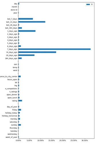
4.1 Average feature importance for the researched variables . . . 23

5.1 Feature importance for the collectively trained model . . . 26

5.2 Product sales for the two companies whose forecasts were affected worst by adding more information, with 156.6% and 69.71% decreases in prediction accu-racy as compared to using only receipt information . . . 27

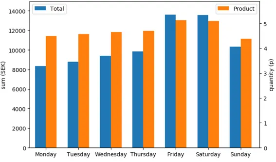
5.3 Average sales per weekday . . . 29

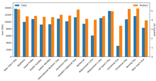
5.4 Average sales on Swedish national holidays . . . 30

5.5 Relationship between the maximum distance to a selected weather station and the forecast improvement from adding weather factors . . . 32

(7)

List of Tables

3.1 Receipt variables . . . 12

3.2 Sales history variables . . . 12

3.3 Selected SMHI parameters . . . 13

3.4 Weather variables . . . 15

3.5 Restaurant variables . . . 16

3.6 Calendar variables . . . 17

3.7 Company reduction . . . 17

3.8 Data set reduction . . . 19

4.1 Comparison of individual and collective training . . . 21

4.2 Average improvement of model sales forecast for all selected companies . . . 22

4.3 The 5 most over- and under-performing variables in the product sales data set . . . 24

4.4 The 5 most over- and under-performing variables in the total sales data set . . . 24

5.1 Effects of adding information on product sales forecasts . . . 27

5.2 Effects of adding information on total sales forecasts . . . 27

5.3 The 5 most and least improved total sales predictions with the addition of weather information . . . 31

A.1 SMHI’s avaliable forecast parameters . . . 39

A.2 SMHI’s avaliable historical parameters . . . 40

A.3 Variables in the product sales data set . . . 41

A.4 Variables in the total sales data set . . . 42

A.5 MAE comparison between individually and collectively trained models for the total sales data set (1/3) . . . 43

A.8 Effects of adding extra information on product sales forecast MAE (1/3) . . . 46

A.11 Effects of adding extra information on total sales forecast MAE (1/3) . . . 49

A.14 Feature importance and Pearson correlation coefficient for the variables in the product sales data set . . . 52

A.15 Feature importance and Pearson correlation coefficients for the variables in the total sales data set . . . 53

(8)

1 Introduction

This report describes an undergraduate thesis project for a Bachelor’s of Science degree in Computer Engineering at Linköping University. The thesis covers 16 ECTS and has been carried out in cooperation with the company Onslip in Linköping, Sweden.

1.1 Motivation

The Internet keeps growing and gains more users every year. In 2017, 49% of the worlds population was connected to the Internet [1]. One effect of this growth is that an increasing amount of data is generated in almost every field. In 2017, an average of 2.5 exabytes(1018) of data was created every day [2], and if current growth continues it is estimated that by 2020, for every person on earth, 1.7 MB of new data will be created every second [3]. According to the International Data Corporation (IDC) the amount of data stored globally is expected to increase from 33 zettabytes (ZB = 1021_{) in 2018 to 175 ZB by 2025 [4].}

Many businesses are now trying to take advantage of this data, with 53% of the nearly 4000 companies asked in a 2017 survey reporting that they are using data analysis tools to affect decision-making, and another 20% expecting to begin in the next two years [5]. In a recent survey of 63 global companies, 62% of respondents answered that they had seen ”measurable results” from investing in ways to analyze their data [6].

Data analysis can be applied to many different areas of business, for example to improve customer experience, forecast demand and streamline operations. According to a survey by Bloomberg Businessweek Research Services, some of the goals for companies that are implementing data analysis tools are to reduce costs, increase profitability, manage risks, optimize internal operations and improve decision-making [7].

There have been several studies performed on the value created by using data for business analytics. According to Chen et. al. [8], using data analysis tools can lead to "unprecedented intelligence on consumer opinion, customer needs, and recognizing new business opportu-nities". A literature review by Wamba et. al. [9], found that data analysis has improved busi-ness performance in several ways, including reduced processing time and improved quality in manufacturing, better insights into consumer needs, customized products and services, improved decision-making, and greater innovation. A case study by Popovic et. al. [10] found that ”when firms utilize more big data analytics, they better forecast previously unpre-dictable outcomes, and improve process performance. As a result, firms realize operational

(9)

1.2. Onslip

process benefits in the form of cost reductions, better operations planning, lower inventory levels, better organization of the labor force and elimination of waste, while they leverage improvements in operations effectiveness and customer service.”

One important source of data is from customer transactions, since this type of data directly reflects customer actions. In 2015, 227.1 billion card transactions were made globally [11], which creates an enormous amount of interesting data for analysis. According to the Swedish Law of Accounting (Bokföringslagen 7 kap. 1-2 §) [12], receipts of every transaction must be kept by the business for at least 7 years, stored in the form, physical or digital, that the business obtained them in. Not having to store physical copies is an advantage for businesses in terms of space and convenience, and the digital copies also give them the opportunity to use data science tools to analyze their activities and improve their results.

1.2 Onslip

Onslip is a Swedish company that sells a cloud-based cash register solution to small compa-nies that run some kind of physical trading, regardless of industry. Onslip offers its own cash register, but it is also possible to use their software on several different platforms. Onslip has customers worldwide who use their product every day. With their solution, customers’ data on completed transactions are automatically saved in the cloud. According to Swedish law, they are obligated to save data on transactions for at least 7 years and therefore have a database with large amounts of data. Currently, Onslip has more than 4 years of data saved that can be accessed by a customer for statistics, but is otherwise not used to provide addi-tional services. They would like to offer more value to their customers by using the saved data.

1.3 Purpose

The purpose of this thesis is to evaluate how predictive machine learning algorithms can be improved, and thereby developing a method for Onslip to analyze large amounts of data automatically. At the end of our work, Onslip will have insights into how they can search for patterns in their stored transactions, and use these to predict the future sales of a product. Onslip will then, for example, be able to provide more accurate sales forecasts or suggest to their customers products that are suitable for promotions.

1.4 Research questions

• How can machine learning algorithms be utilized to predict future sales? • Which factors affecting sales have an impact on the accuracy of predictions?

1.5 Limitations

• This work will focus on producing a solution for one specific area of business, restau-rants, and not one general solution for all of Onslip’s customers.

• This work will not analyze algorithms or frameworks in depth, but will simply choose existing solutions based on previous research.

(10)

2 Theory

2.1 Automated forecasting

There are many applications for predicting future demand of the products and services that a business is supplying. Forecasts are used throughout most industries for planning produc-tion and business operaproduc-tions, purchasing materials, managing inventory, scheduling work hours, advertising, and much more [13]. Traditional forecast methods have mostly been based on opinions of experienced employees or on statistical analysis of previous history, but in recent years machine learning algorithms have been applied to this area with much suc-cess [14]. Using machine learning techniques instead of relying on human expertise means that a business can spread and hold on to knowledge that only some employees have, and by automating the process it is possible to apply forecasting methods on a much larger scale.

2.2 Data mining and machine learning

Data mining is the process of discovering patterns in data, by using methods and techniques from machine learning and statistics [15]. This process is usually automated and performed on databases. Much of data mining involves the application of machine learning tools to extract information from the data and find underlying structures. The goal is to find gen-eral patterns that explain something about the data, and use these to guide future decision making.

In the context of data mining, machine learning can be explained as creating structured descriptions of data [15]. The form of these descriptions depend on the algorithm used to create them, and can consist of, for example, mathematical functions, rule sets or decision trees. The descriptions represent what has been learned from the data, and are used to make assumptions about new and previously unseen data. By looking at what attributes of the data had the biggest impact in the creation of the descriptions, it is also possible to verify suspected relationships, or see other patterns that may have been unknown earlier.

The most common way of acquiring these descriptions is by looking at examples [15]. The machine learning model is provided with input data, and the objective is to find the best transformation of input data into corresponding output data. In unsupervised machine learning, the model does not know the output in advance, while supervised learning models are given examples in pairs of inputs and correct outputs. Compared to unsupervised

(11)

learn-2.3. Decision trees

ing, a supervised model needs to receive feedback about how close its assumptions are to the real answers, and it learns by trying to minimize the error produced by the feedback. A classification model attempts to predict output data ranging over a discrete interval, while a regression model makes predictions for continuous data.

2.3 Decision trees

A decision tree is a data structure commonly used to represent a machine learning model’s knowledge. At each internal node of the tree, the data set is split in two parts based on the values of one input variable [16]. Growing the tree involves deciding which variable to use for the split, and what value of the variable to split the data on. This is done through exhaustive search of the different variables, meaning that all possible splits are considered, and the split that produces the lowest error is chosen. The amount of splits to be considered can be reduced by using heuristic search and function optimization techniques.

The leaves of the tree contain the model’s prediction. In a classification model the values in the leaves are different categories, and in a regression model a leaf’s value is the mean of every data point in the training set that leads to this leaf. A few of the steps involved in creating a decision tree from a data set with two-dimensional input can be seen in Figure 2.1.

Figure 2.1: Selected steps in the creation of a decision tree, and its corresponding partitioning of the training set

Decision trees with many variables can grow very complex and often have problems with over-fitting: when the model is too specialized to the training set that it looses accuracy when applied to other, more general problems [16]. One way to avoid this is to keep the tree as simple as possible. Typical criteria of when to stop growing the tree are when it has reached a maximum depth, when there are a certain number of leaves, or when the error reduction is less than a threshold value. It is also possible to prune the tree afterwards, a process that removes a split node from the tree. A node is removed if its elimination either reduces the error, or does not increase the error too much while reducing the size of the tree sufficiently.

(12)

2.4. Decision forests

2.4 Decision forests

The process of applying several machine learning models to the same problem and combining their results is called ensembling [16]. This approach is based on an idea from probability theory in mathematics, that, if some independent predictors are correct with a probability higher than 50%, the combined prediction has a higher probability of being correct than any single predictor. If the ensemble consists of decision trees, it is called a forest.

There are two different ways of creating forests, bagging and boosting. Bagging involves sampling subsets of the training data and creating new independent trees for each subset, so that they hopefully reflect different aspects of the data. These trees are usually grown from small subsets to reduce their similarity, but allowed to grow deeper to be able to discover more complex patterns. The final prediction is decided using all of the models, for example by taking the most common, mean or median value.

In boosting, the trees are not independent but are instead created sequentially based on the error of the previous trees [16]. By removing the already captured patterns, the following tree can focus more on finding new aspects of the data that are harder to discover. One issue with this approach is that, because the trees do not train on the whole training set, they are more likely to find patterns that do not reflect the actual data. Therefore, the trees are usually not allowed to grow too deep, and are sometimes even kept to only one split.

The boosting algorithm starts by creating an initial model that roughly approximates the training data, usually by simply using the minimum or mean value [17]. The next step is to calculate how much the approximation differs from what is expected. The result is a set of vectors, one for every point in the training data, called the residual vectors, that describe in which direction and how far off each estimate is from its target. A second model is then trained to approximate these residuals. The new model’s estimate of the residuals is added to the first model. The differences from the expected results are once again calculated, and another set of residual vectors are produced. This continues until a certain number of models have been trained, or the algorithm stops making sufficient progress.

The combined prediction ˆy of a boosted model can be represented as the sum of all indi-vidual model’s predictions fi(x).

ˆy=

N ÿ i=1

fi(x) =F(x) (2.1)

The current boosted model at step i can therefore be described as the previous boosted model combined with the current individual model.

Fi(x) =Fi´1(x) + fi(x) (2.2) We can show the usefulness of boosting machine learning models with a simplified exam-ple using the function y=5+x+sin(x), seen in figure 2.2a. The first model looks at where the curve intercepts with the y-axis at(0, 5), and so approximates the function as f1(x) =5, shown together with the original function in figure 2.2b. The errors produced after the first model’s predictions are shown in figure 2.2d. The second model receives this curve as its in-put and sees that it can be represented quite well with a simple linear function, matching com-pletely at every „ 3.14 steps. It therefore approximates the curve as f2(x) =x, which is added to the previous function, as can be seen in the figure 2.2c. The third model, again, is trained on the aggregated error produced by the predictions from the previous models, shown in figure 2.2e. The model recognizes the patterns of a sine wave and adds f3(x) =sin(x)to the approximation, which eliminates the error completely, as the boosted models have found the correct function. In real use cases the input is not a single variable, the function is often much more complex, requires many more models to solve, and can not be exactly approximated, but the process remains the same.

(13)

2.5. Gradient boosting

(a)y=5+x+sin(x) (b)y=5+x+sin(x), ˆy=5 (c)y=5+x+sin(x), ˆy=5+x

(d) Difference between the two functions above

(e) Difference between the two functions above Figure 2.2: Boosting example

2.5 Gradient boosting

Gradient descent is an optimization technique used to minimize functions by taking small steps in the direction where the slope of the function is steepest [17]. This is done by first calculating the gradient∇of the function f at the current point using its partial derivatives.

∇f(x) =    B f (x1) Bx1 ¨ ¨ ¨ B f (xN) BxN  

 wherexis a vector with N dimensions (2.3) The gradient represents a vector with the direction of the steepest slope, and a length propor-tional to the steepness of the slope.

The second step of gradient descent uses the gradient to calculate the next point to inves-tigate. To avoid going too far and missing the actual minimum, only a part of the gradient is applied. How much is controlled with the learning rate factor γ.

xi+1=xi´ γ ¨∇f(xi) (2.4)

This concept is used in the gradient boosting machine learning algorithm to minimize the error function in a similar way; by calculating the negative gradients and using them to train the next model.

ˆyi+1= ˆyi+γ(´∇e(y, ˆyi)) (2.5)

2.6 XGBoost

In 2016, Tianqi and Carlos [18] published their study of a tree boosting system called eX-treme Gradient Boosting, or XGBoost (XGB). XGBoost is an effective implementation of the gradient boosted decision trees algorithm. The framework is fast and has both CPU and GPU implementations. It also supports multi-thread parallelism, which makes it even faster.

(14)

2.7. Related work

XGBoost has two types of split decision algorithms, a pre-sort-based algorithm called Exact Greedy, which is used by default, and a histogram-based algorithm. Exact Greedy first sorts each feature before enumerating over all the possible splits and calculating the gradients. Each tree that is created is given a score that will represent how good it is. The trees are built sequentially so that the result of the previous tree can be used to help build the next tree.

A common problem that can occur when using machine learning techniques on large data sets is that all the values may not fit in the CPU cache, which can greatly increase computation times. XGBoost has solved this problem with a cache-aware algorithm and therefore achieves better performance than similar machine learning frameworks when applied to large data sets. This makes XGBoost a great tool when computation resources are limited.

Another advantage of XGBoost is that it has implemented a way to handle missing values, which is another common problem in machine learning. XGBoost solves this by using a default direction in each split, which will be selected if values are missing for this feature.

2.7 Related work

Predicting future sales of food with machine learning is not a new subject, however much of the research in this area has focused on forecasting for retail grocery stores.

A survey by Tsoumakas [19] reviewed 13 research papers on machine learning in food sales predictions. Only in one of these articles had a restaurant been researched. The author found that most forecasts made daily predictions, while some used longer time spans up to weeks and even per quarter. The most commonly predicted output variable was amount sold in piece or weight, followed by monetary amount. According to the survey, the most common input variables to the machine learning algorithms are historical sales figures for different intervals. These can be, for example, the amount sold on this day last week or year, and average sales for the last week or month. Other usual inputs are characteristics of the date and time, such as the day of the week, month of the year, and if the date is a holiday. Some inputs that occur less often in these papers are external factors that would require collecting data from outside the company, for example financial, social and weather factors, and different types of events occurring in the vicinity of the business. According to the author, there exists an unexplored opportunity to make use of product information as input variables to predict demand for multiple products with the same model.

Doganis et. al. [20] combined a neural network with a genetic variable selection algorithm and tried to predict the daily sales of fresh milk for a dairy producer in Greece. They created additional input variables from the provided sales data, similar to what was used in current forecast methods. The examined variables were sales figures from the previous week of the current year, the previous week of last year, the corresponding day of last year, and the per-centile change in sales from the previous year. The authors compared the forecast accuracy of the neural network to other linear regression algorithms, and found that the neural network, which was the only model provided with the additional variables, had an average error of less than 5% compared to 7-10% for the other models. The most useful input variables identi-fied by the variable selection algorithm were the sales on the previous day and the same day last week.

Žliobait ˙e et. al. [21] predict the weekly sales of products for a food wholesaler in the Netherlands. They start by categorizing products into predictable and random sales patterns. This is performed by creating variables from the products’ sales history, including variations of the mean and median values, quartiles, and standard deviation, and feeding these to an ensemble of classification models that decide the product category by majority vote. Fore-casts are then made for the products with predictable sales patterns, using an ensemble of predictive algorithms. The input variables provided to the predictors in this study were daily product sales, average weekly product sales, daily total sales, product promotions, holidays,

(15)

2.7. Related work

season, temperature, air pressure and rain. The most used variables were the product related variables, the season, the temperature and one of the included holidays. The results show that the presented solution outperformed the baseline moving average forecast method, and by reducing the threshold of which products were categorized as predictable, the accuracy could be improved further. They also discuss the possibility that the classification model can be excluded and its input variables incorporated directly into the prediction model.

˙I¸slek and Ö˘güdücü [22] developed a forecasting method for a Turkish distributor of dried nuts and fruits. The company has almost 100 main distribution warehouses, which have their own sub-distribution warehouses. The input data included warehouse related attributes, for example location, size, number of sub-warehouses and transportation vehicles, selling area in square meter, number of employees and amount of products sold weekly, as well as product information such as price and product categories. Their solution first used a bipartite graph clustering algorithm to group warehouses with similar sales patterns, and then a moving average and Bayesian network combination model to predict the weekly sales of individual products at each warehouse. The authors evaluated the forecast accuracy for three differ-ently trained models. One handled all of the warehouses grouped together, one used clusters of main warehouses, and the last was given sub-warehouse clusters. The clustering algo-rithm generated 29 different main warehouse clusters, and 97 clusters for the sub-distribution warehouses. The results showed that the error rate of the model dropped from 49% without clustering, to 24% with main distribution warehouse clusters, and 17% with sub-distribution warehouse clusters.

Liu and Ichise [23] performed a case study of a Japanese supermarket chain, in which they implemented a long short-term memory neural network machine learning model with weather data as input parameters to predict the sales of weather-sensitive products. They used six different weather factors: solar radiation, rainfall precipitation, relative humidity, temperature, and north and east wind velocity. Their results show that their model’s predic-tions had an accuracy of 61,94%. The authors mention plans to improve their work in the future by adding other factors known to affect sales, such as area population, nearby com-petitors, price strategy and campaigns.

An early research paper that focused on restaurants was written by Takenaka et. al. [24], who developed a forecasting method for service industry businesses based on the factors that interviewed managers took into account when forecasting manually. The examined fac-tors include the weekday, rain, temperature and holidays. They found that their regression model could provide more accurate predictions for a restaurant in Tokyo than the restaurant manager.

In a study from 2017, Bujisic et. al. [25] researched 17 different weather factors and their effects on restaurant sales. They analyzed a data set consisting of every meal sold at a restau-rant in southern Florida during 47 weeks, from March 2010 to March 2011. Their results showed that weather factors can have a significant effect on sales of individual products, however not all products are affected by the weather, and the same weather factor has differ-ent effects on differdiffer-ent products. They also found that the most important weather factor was the temperature, followed by wind speed and air pressure.

Xinliang and Dandan [26] used a neural network to forecast daily sales of four restaurants located at a university campus in Shanghai. The input variables provided to their model were the restaurant’s name, the date, the teaching week, the week of the year, if the date was a holiday, temperature, precipitation, maximum wind speed, and 4 different search metrics from Baidu, China’s largest search engine. The authors found that the name of the restaurant was the most important variable, followed by the teaching week, holiday, and one of the Baidu variables. The weather factors were shown to have low importance to the model, with temperature slightly above the other two.

Ma et. al. [27] predicted future visitors to restaurants using a mix of K-nearest-neighbour, Random forests and XGBoost. Their data was obtained from large restaurant ordering sites, and included 150 different restaurants. To compare different restaurants, the authors

(16)

con-2.8. Forecast accuracy metrics

structed several input variables from restaurant attributes such as a unique ID, latitude, lon-gitude, genre, and location area. The results showed that XGBoost was the best individual model, and that the most important variables were the week of year, mean visitors, restaurant ID and maximum visitors.

Holmberg and Halldén [28] researched how to implement machine learning algorithms for restaurant sales forecasts. To improve the accuracy of the predictions, they included vari-ables based on sales history, date characteristics and weather factors. The weather factors used for their model were temperature, average temperature of the last 7 days, rainfall, min-utes of sunshine, wind speed, cloud cover, and snow depth. They examined two different ma-chine learning algorithms and found that the XGBoost algorithm was more accurate than the long short-term memory neural network. The date variables were the most significant and the weather factors had the least impact. They also found that the daily sales were weather de-pendent for all of the researched restaurants, and that introducing weather factors improved their models’ performance by 2-4 percentage points. They suggest that continued work could be to create more general models that can make predictions for multiple restaurants, possibly by categorizing different restaurants based on features such as latitude/longitude, inhabi-tants, size of restaurants, and opening hours.

From these studies a few key facts can be extracted. While models that perform time series forecasting by default have access to previous sales figures, results can be improved by emphasizing certain patterns with their own input variables. Which input variables prove to be most important seems to be different in every study, and depend on the variables included, and the behaviour of each restaurant’s customers. Some variables are however more likely to have a greater effect, with variables related to date and sales figures more often represented in the lists of most important variables. Almost all of the early studies make use of some kind of neural network architecture, but in more recent papers the use of XGBoost becomes more popular, and it has been shown to be one of the best performing algorithms for prediction and forecasting problems [19, 27–33].

2.7.1 Weather’s effects on sales

Several studies have shown that the weather can have a significant effect on business, both seasonal and day-to-day. Murray et. al. [34] mention three key factors as the most important reasons. Firstly, the weather impacts an individual’s will to go outside, and thereby that per-son’s opportunity to make a purchase. If it is cold, or it rains or snows heavily, you are much more likely to stay home. Additionally, some weather factors and seasonal changes have ef-fects on people’s mood, which in turn afef-fects their willingness to spend money. The lower levels of sunlight during the winter months can lead to Seasonal Affective Disorder [35], es-pecially in the northern parts of the world [36]. Lastly, some products are very dependant on the season and can experience huge variations in sales over the year. Drinks, for example, sell much more during the summer.

2.8 Forecast accuracy metrics

There are a wide range of available methods for how to statistically evaluate the accuracy of a forecast. These all have different complexity and advantages, and usually there is no metric that is best in every case [37]. The most appropriate measurement depends on the attributes of the input data and the predicted values, and should be chosen based on each individual situation. Some metrics are more sensitive to outliers in the data, where one bad prediction can have a significant impact on the overall performance. Others are based on the scale of the predicted values, and can not be easily compared against each other. Some do not have meaningful interpretations, and it can be hard to understand what they are meant to show.

A relative accuracy metric first uses one baseline forecast method, and then compares other predictions against the performance of the baseline. This metric has the advantage of

(17)

2.8. Forecast accuracy metrics

being independent of the scale of the predicted values, and only measures the difference in prediction accuracy.

2.8.1 Mean absolute error

The mean absolute error (MAE) is a popular accuracy metric because it is easy to under-stand. It simply measures the absolute difference between the real and predicted values. It is calculated using the formula below.

1 N¨ N ÿ i=1 |yi´ˆyi| (2.6)

(18)

3 Method

3.1 Raw data

For this study, Onslip provided a snapshot of one of their production databases, with data of every transaction processed from 2015-01-01 to 2019-05-07. Because Onslip’s customers operate in various industries, it was discussed that focusing on one type of business could make it easier to achieve results. If this project was successful, the insights gained could then be applied to more businesses. The restaurant category was chosen as it was the one with the most customers, and the most data.

The data used is obtained from the receipts of transactions in a business category that On-slip calls "Small ticket Food&Beverage". This group contains restaurants that receive orders of on average 5 products, and includes for example pizzerias, thai- and sushi-restaurants. These are Onslip’s main target group and constitutes most of their customers.

The data included 11 481 129 individual transactions, of in total 34 163 817 items, for a total amount of 1 854 132 529.49 SEK. 374 unique companies and 59 076 different products were identified.

3.2 Receipt data

One data point for a transaction contains all the information printed on the receipt at the time of sale. Some of these fields are required by Swedish law, such as the date, time, items, monetary amount and tax rate of the purchase, and the organization number and address of the selling business. Other fields contain information included by the business, as Onslip allow their customers to add their own custom information to the receipts.

From the raw data, the name and address of the business was extracted and, for every purchase, the date and time, and individual items, quantities and prices. Each company’s extracted data is then arranged by a combination of item, price and date, and added together in one data set that shows the quantity of each product sold per day per price. An addi-tional data set is created by summing up the sales for all products using the product, price and quantity variables, to show the total monetary amount sold at each restaurant per day. Because all predictions are made on a per day basis, the time stamps are not included in any of the data sets. Table 3.1 shows all variables that were extracted from the receipt data.

(19)

3.3. Sales history data

Table 3.1: Receipt variables

Variable Description Type Data set

day The day of the month of the date of sale Integer Both

id The ID of a product Integer Product sales

month The month of the year of the date of sale Integer Both

price The sale price of a product Float Product sales

quantity The total amount of a product sold on this date Integer Product sales store-address The address of the restaurant String Both

store-name The name of the restaurant String Both

sum The total amount in SEK sold on this date Float Total sales

time The time of day of the sale Time stamp None

year The year of the date of sale Integer Both

3.3 Sales history data

Information about previous sales were calculated from the extracted receipt data. These vari-ables were constructed based on results from previous research by Doganis et.al. [20].

The data sets are first separated by either unique product and price combinations in the product data set, or by store-name in the other case. The calculations are performed with the operations shift, which shifts all data points the specified number of times, rolling, which creates fixed-size rolling windows, and mean, which calculates the mean value in the given range. For data points where the values were shifted out, the first occurring value was used to fill the range backwards. When there was not sufficient data for the rolling operations, the mean value of the entire data set was used instead. The sales history data consisted of 14 additional variables, seen in Table 3.2 below.

Table 3.2: Sales history variables

Variable Description Type

1_days_ago The amount sold 1 day before the date of sale Float/Integer 2_days_ago The amount sold 2 days before the date of sale Float/Integer 3_days_ago The amount sold 3 days before the date of sale Float/Integer 4_days_ago The amount sold 4 days before the date of sale Float/Integer 5_days_ago The amount sold 5 days before the date of sale Float/Integer 6_days_ago The amount sold 6 days before the date of sale Float/Integer 7_days_ago The amount sold 7 days before the date of sale Float/Integer 14_days_ago The amount sold 14 days before the date of sale Float/Integer 28_days_ago The amount sold 28 days before the date of sale Float/Integer 364_days_ago The amount sold 364 days before the date of sale Float/Integer mean_last_7_days The mean amount sold in the 7 days before the date of sale Float/Integer mean_last_14_days The mean amount sold in the 14 days before the date of sale Float/Integer mean_last_28_days The mean amount sold in the 28 days before the date of sale Float/Integer mean_last_364_days The mean amount sold in the 364 days before the date of sale Float/Integer

3.4 External data collection

Three different key categories of external data have been identified as being of interest in earlier research: weather factors [21, 23, 24, 26, 28, 29, 31], attributes of the restaurants or products [22, 26, 27, 29, 33], and date characteristics [21, 23, 24, 26–31, 33]. This information is gathered from different publicly available sources, in the ways described in the following sections.

(20)

3.4. External data collection

3.4.1 Weather data

To obtain the weather information, the Swedish Meteorological and Hydrological Institute (SMHI) was chosen as the source. They offer daily statistics about the weather, such as pre-cipitation, temperature, wind speed, and more. SMHI offers both historical weather infor-mation several years back as well as forecasts for the next ten days. With the help of SMHI’s Application Programming Interface (API), that information can be retrieved easily. To fetch weather information for a specific area a position is needed.

Which weather factors to use was decided by comparing the list of available parameters for historical data to the parameters in forecasts1_{. The historical parameters were obtained} from an API call while the forecast parameters were taken from SMHI’s API documentation. Get all weather types available in the historical data:

https://opendata-download-metobs.smhi.se/api/version/latest/ parameter.json

Get all weather types available in the forecasts:

https://opendata.smhi.se/apidocs/metfcst/parameters.html

Eight parameters that belonged to both sets were identified: air pressure, air temperature, rainfall, relative humidity, visibility, wind direction, wind gust, and wind speed. Rainfall was not found directly in the forecast parameter list, but could be calculated by checking if the precipitation category was rain and then multiplying the mean precipitation by 24. Unfortunately, data could not be obtained for all the requested parameters and intervals and were therefore not used. The remaining weather factors selected for this work are displayed in Table 3.3.

Table 3.3: Selected SMHI parameters

Parameter Weather type Attribute Measured Interval

2 Air Temperature Average 1 time/day

4 Wind Speed Average 1 time/hour

5 Rainfall Sum 1 time/day

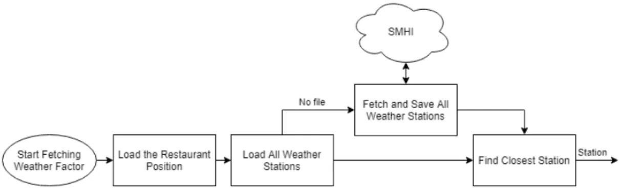
SMHI has two different APIs, one for retrieving older weather data and one for current and future weather data. To retrieve older weather data, a weather station must be specified as an argument when using the API. The other only needs a position in longitude and lat-itude. The process to retrieve old weather data is divided into two parts. First, a list of all stations that have data for the chosen weather factor is fetched and saved. If there is a file containing all the weather stations for the selected weather factor, it is loaded instead. This list is searched through and the distance to each station is calculated to find the one that is nearest to the restaurant’s location. Figure 3.1 shows a flow diagram of how the first part is done. The call that is used to fetch all stations is shown below, where {parameter} is replaced with a parameter from Table 3.3.

Get all stations’ positions and IDs:

https://opendata-download-metobs.smhi.se/api/version/latest/ parameter/{parameter}.json

In the second step, the weather station is used as a parameter to call SMHI’s API and request the data. The data is received as a Comma Separated Values (CSV) file. Some rows and columns only contain comments or unnecessary information and are therefore removed.

1_{The complete lists of SMHI parameters can be found in the Appendix, in Table A.1 on page 39 and Table A.2 on}

(21)

Figure 3.1: Flow diagram of the process to find the closest station

Figure 3.2 shows how this is done. Also shown below is the call that is used to fetch historical weather data, where {station} is the ID of the chosen station.

Fetch historical weather data from a specific station:

https://opendata-download-metobs.smhi.se/api/version/latest/

parameter/{parameter}/station/{station}/period/corrected-archive/data.csv

Figure 3.2: Flow diagram of the process to fetch weather data for the given station The historical weather data is obtained in two different time periods: corrected archive, which contains data from the beginning of collection until about three months before the current date, and latest months, which has data for the latest four months. This caused some overlap in the data, so because, according to SMHI, the corrected archive is more accurate, when there were multiple data points for the same day, the ones obtained from the archive were selected.

When obtaining the weather information, several problems arose with how the stations had saved their data, for example that many stations:

• Did not save weather history at all.

• Had stopped saving data several decades ago. • Had not saved data continuously.

• Had saved data with different time intervals.

To solve these problems, it was first checked whether the nearest station to the position had any weather data available. Instead of excluding the restaurant if the weather station had no information, the next nearest weather station was examined until a weather station which had weather history was found. The station must also have data for the dates in the requested interval. If the station did not have weather history for those dates, then the next weather station was searched. This was done because it was believed that slightly higher distances

(22)

would not affect the weather too much. This is analyzed further in the discussion chapter. Once a station had been found with weather history for the dates sought, the downloaded weather information was processed. For parameters that provided more than one data point per day, the mean value of all points was calculated and used instead.

The final weather variables used in this project are shown in Table 3.4. Table 3.4: Weather variables

rain The total amount of rainfall in millimeters on the date of sale Float temp The average air temperature in degrees Celsius on the date of sale Float wind The average wind speed in meters per second on the date of sale Float

3.4.2 Google Maps data

Initially, the plan was to include as much business information as possible about the restau-rants, in order for the model to be able to distinguish their unique sales patterns. This hy-pothesis was supported in previous research [21, 22, 27]. However, because Onslip do not require their customers to fill in any information specific to their business except for what is demanded by law, there was no information that was available for every company used in this study.

Instead, since there had been some success in using information obtained from Internet search engines as business indicators [26], and because use of public information would in-crease replicability, the option of using Google Maps as an external information source was explored. Variables were constructed based on the information available from Google, which was retrieved through their Web Services API using the Python library googlemaps2.

In the first step of the retrieval process, one API call for every address found in the receipt data is made to the Geocode service, with the address and name of the restaurant. This returns a list of locations that match all or parts of the search string. To filter out irrelevant results such as the street, city block and municipality, which would always be found as long as the address is legitimate, search results that only have the types ’street address’, ’premise’ or ’political’ are removed. Because all of the companies included are located in Sweden, any results found outside of Sweden are also discarded. After the filtering, the PlaceID of the location is extracted from the search result. This is an ID internal to Google Maps that uniquely identifies the specific location.

In the second step this PlaceID is used in a call to the Place service, which returns the public information stored for this location. From this information a few fields are extracted directly, including its latitude and longitude, star rating and number of ratings, while other fields go through more processing. Some calculations are performed on the opening hours of the business, and the number of hours open each day of the week is saved, along with if the restaurant was open during lunch (defined as 11:00-13:00) or dinner (17:00-19:00).

The latitude and longitude values, and the city where the business is located are used in an additional API call to the Directions service, to calculate the walking distance from the location to the city center, which is also saved.

Lastly, an API call to the Places service is made to find the number of nearby competitors. After removing too general types such as ’store’ and ’establishment’, a search is done with the types of the location, and its latitude and longitude values. Google does not currently support only including results within a certain radius, so an additional filtering of the results is therefore done to calculate the number of competitors within 1000 m.

The restaurant’s information is saved in JSON format for easy access and later added into the data set by using the address of the restaurant where the sale was made to find the correct

(23)

3.5. The combined data sets

file and adding it to the saved information for each sale. When merged with the sales data, there are in total 9 additional variables related to the business taken from the Google Maps API, as can be seen in Table 3.5.

Table 3.5: Restaurant variables

distance_to Walking distance in meters from the restaurant’s location to the Integer _city_center geographical center of the city

hours_open The number of hours the restaurant was open on the date of sale Float

lat Latitude value of the restaurant’s location Float

lng Longitude value of the restaurant’s location Float

open_lunch If the restaurant was open during lunch (11-13) on the date of sale Boolean open_dinner If the restaurant was open during dinner (17-19) on the date of sale Boolean n_competitors The number of restaurants with the same types within 1000 meters of Integer

the restaurants’s location

n_ratings The number of ratings received on Google Maps Integer

rating Average rating received on Google Maps Float

3.4.3 Product data

As with the business information, adding any information about specific products, for exam-ple their purchase cost, ingredients or sale price, is entirely optional for Onslip’s customers, and was missing for almost every company. Information of this kind is also not publicly available, and would involve crawling each individual company’s website, in the case that they have one, hoping that every product is listed. It was therefore not feasible to add any additional product variables to the data sets.

3.4.4 Calendar data

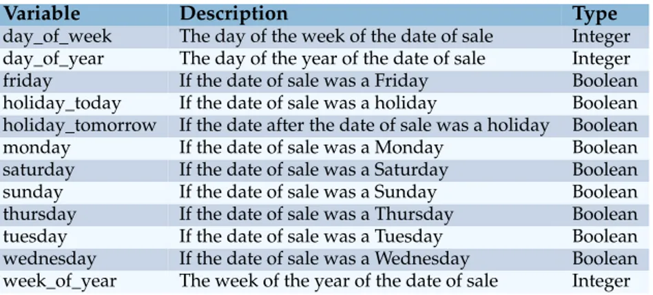
The date from the receipt was used to add more variables related to the date of sale. The date is first converted to a Datetime object in Python with the datetime module3. With this, several variables are created, such as the weekday, the day of the year, and the week of the year. Because it was believed that the weekday variable would have a significant impact, each weekday was also represented with individual variables.

The Datetime object is also used together with the holidays library4to create additional variables representing if the current or following date is a holiday. As every Sunday is a holiday (or ”red day”) in Sweden, and the library methods reflect this behavior, the name of each holiday had to be checked, and any dates that were only tagged with ’Sunday’ were not counted as holidays. There were 11 calendar variables added, shown in Table 3.6.

3.5 The combined data sets

The weather, calendar, restaurant and sales history data were combined with the receipt data to create one large data set with all the examined variables. The sales history data was merged on the date of sale and either product ID and price in the product data set, or the restaurant’s address in the total sales data set. Weather data was added using the date of sale and the ad-dress of the restaurant, while calendar and restaurant data were simply merged on the date of sale and restaurant address respectively. Any data for dates that did not have corresponding dates in the receipt data was not included. If any external data could not be found for a com-pany, regardless of the reason, this company was not included. The combined product sales data set contains 45 variables, and the total sales data set has 43. A list of all the variables is

3_{https://docs.python.org/2/library/datetime.html} 4_{https://pypi.org/project/holidays/}

(24)

3.6. Company selection

Table 3.6: Calendar variables

day_of_week The day of the week of the date of sale Integer day_of_year The day of the year of the date of sale Integer

friday If the date of sale was a Friday Boolean

holiday_today If the date of sale was a holiday Boolean holiday_tomorrow If the date after the date of sale was a holiday Boolean

monday If the date of sale was a Monday Boolean

saturday If the date of sale was a Saturday Boolean

sunday If the date of sale was a Sunday Boolean

thursday If the date of sale was a Thursday Boolean tuesday If the date of sale was a Tuesday Boolean wednesday If the date of sale was a Wednesday Boolean week_of_year The week of the year of the date of sale Integer

attached in the Appendix, and can be found in Table A.3 on page 41, and Table A.4 on page 42.

3.6 Company selection

Not all the companies in the data that was provided by Onslip could be included in this study, mostly due to missing or incorrectly filled out fields in the information printed on the receipts. Some companies had names or addresses with spelling errors, and others had addresses that did not match the location of the restaurant. Because it would take a long time to individually inspect all transactions for spelling mistakes or manually search for the restaurant’s location, it was decided to discard these companies. There were also several fabricated companies, that are used internally by Onslip during testing. Of the initial 374 companies, 116 did not have a legitimate address, and their positions could not be confirmed. This meant that there was nothing that could be used when fetching weather data from SMHI and restaurant data from Google Maps. Their transactions were therefore not included when training the models, and no forecasts were made for these companies.

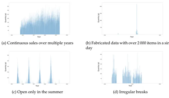
After the data extraction and external data collection processes, 258 companies remained. In an effort to improve the predictions of the model trained with every company’s data, these companies were analyzed by plotting their sales over time and categorized as shown in Table 3.7. In previous papers on this topic, it is mentioned that grouping data sources with similar sales patterns is believed to improve the model’s performance [22, 28].

Table 3.7: Company reduction

Description Companies

Missing data 116 Very few days 22

Only summer 18

Less than one year 57 Irregular breaks 31

Selected 130

Total 374

Figure 3.3 shows examples of different identified sales patterns. First, any companies that did not have sales for more than 10 days were identified. Because they would not have enough data to find meaningful patterns, they were removed from the data sets. Then, it was discussed that companies that are open for just a few weeks during summer should be trained together in a separate data set, since they only had small amounts of data and some of the examined parameters, such as month, temperature, and holidays, did not show much variance. Companies that did not have one full year of sales were also not included, as it was

(25)

3.6. Company selection

(a) Continuous sales over multiple years (b) Fabricated data with over 2 000 items in a single day

(c) Open only in the summer (d) Irregular breaks Figure 3.3: Examples of companies with different sales patterns

believed that if a date had not occurred twice it would be difficult to compare any seasonal impact of the examined parameters. Lastly, companies that had large gaps in their data with irregular intervals were filtered out. This did not include companies that were closed on the same days every year, for example during Christmas and New Year, or a few weeks of summer vacation.

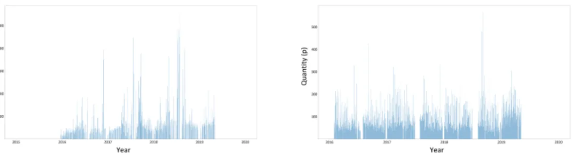
Figure 3.4a shows the product sales quantities over time for all 374 companies that were initially extracted from the receipt data. It shows that the sales are increasing over the years and have peaks in the middle of each year. The increasing sales are due to the increasing number of Onslip´s customers, and the peaks are mostly from restaurants that are only open during the summer. Figure 3.4b shows the same graph for the 130 companies remaining after the selection process. When comparing this figure to Figure 3.4a, the new data set has a much more even distribution, and the peaks in the middle of each year are almost gone.

(a) All 374 companies provided (b) The selected 130 companies Figure 3.4: Total number of products sold per day from January 2015 to May 2019 At the end of the selection process, 130 companies had been identified that had mostly continuous sales over more than one year. Although this meant that only about 35% of the initial companies remained, they still accounted for almost 70% of the transactions, as shown in Table 3.8.

(26)

3.7. Model implementation

Table 3.8: Data set reduction

All Selected

Transactions 11 481 129 7 955 897 Items 34 163 817 17 659 400

Products 59 076 29 210

Amount 1 854 MSEK 1 125 MSEK

3.7 Model implementation

The combined data sets were split into training and test sets. The test set, which consisted of the last 28 days of the data set, was saved for evaluation. The other days were used to train an XGB regression model. In order to use the regressor, all variables must be converted to either integers, floating point numbers or Boolean values. The name and address of the restaurant were therefore replaced with a unique ID. The prediction target was also separated from the other variables.

The regressor is initialized with parameters that decide how the training will be per-formed. In this implementation, the maximum allowed number of trees, the maximum al-lowed depth of a tree, and the learning rate were changed from the default values. The values used instead were found by creating several models with different parameter settings and comparing their performance. The values that occurred most often in the top perform-ing models were selected. Findperform-ing the best parameter settperform-ings took more than one day per company. Due to the large number of companies it would be too time-consuming to find the optimal parameters for every company and therefore the same parameter settings were used to train every model.

To avoid overfitting, the early-stopping functionality of XGB was used. This lets the model evaluate its progress after each successively generated tree, and stop the training if there is no improvement. In order to use early-stopping, a validation set needs to be provided, which is used to measure the accuracy of the current model. 10% of the training set was randomly chosen and set aside for validation. The training was stopped if a better tree could not be generated for 100 iterations.

When a model has been created it can be saved to a file, and later loaded to continue training or make predictions. An extract of the code to implement the model can be seen in Listing 3.1.

x_train, x_val, y_train, y_val = train_test_split(x, y, test_size = 0.1)

model = xgb.XGBRegressor( max_depth = 3,

learning_rate = 0.01, n_estimators = 6000, booster = ’gbtree’, objective = ’reg:squarederror’) model.fit( X = x_train, y = y_train, early_stopping_rounds = 100, eval_metric = [’mae’], eval_set = [(x_val, y_val)])

(27)

3.8. Evaluation

3.8 Evaluation

To evaluate the performance of a model, its sales forecast was compared to the actual sales values that had been extracted from the receipt data. The model’s accuracy was measured using the MAE metric, which was chosen because it could be easily interpreted and explained to a person without knowledge of statistical analysis methods. Since the different forecasts are only compared against each other to measure their relative performance, the main concern was to obtain the results in a way that would enable good visualization for Onslip and its customers.

For each product or restaurant, the latest 28 days were withheld from the model during training and used as a test data set. It was discussed that 28 days would be a good time frame to visualize the forecast for Onslip and its customers. When using the combined data sets to evaluate the model for specific companies, only the last 28 days of sales for that company was put aside. Before producing any forecasts, the prediction target column (quantity in the product set and sum in the total sales set) was removed from the test data. The model was then given the reduced data points to make individual predictions on how much would be sold on each day with the given parameters. No predictions were made for days in the test set that did not have any sales, since a restaurant would not try to forecast their sales on a day when they would not be open. The forecast was then compared to the real values, and the MAE for the whole test set was calculated.

One initial evaluation was performed to determine if it was better to train a model on all the available data, or only use data generated by each company. Because of the amount of time it would require to compare every company with both data sets, only the total sales set was used. First, for every company, the combined data set, excluding that company’s last 28 days of sales, was used to train individual XGB regression models. The models then tried to forecast the total sales amounts for the company on those days, and their predictions were saved and evaluated. Then, also for every company, additional regressors were trained using only that company’s data, except for the last 28 days. New forecasts were made for the total sales amounts, which were also saved and evaluated. The two forecasts were then compared and the relative difference in MAE was calculated for every company. Lastly, the mean difference for all companies was calculated.

To evaluate the impact that the different parameters had on the predictions, a similar procedure as the one just described was used to train several regression models. Both data sets were used in this evaluation. For each company, for both the product and total sales data sets, a model was first trained without any additional variables added. The only available input parameters for these models were the dates and the restaurant’s ID, and either the product ID, price and quantity, or the total sales amount. The predictions made by the first models were saved and the MAE was calculated, so it could be used as a baseline to compare against later models that would be given more variables.

Because there were too many variables to examine them all individually5_{, the parameters} were evaluated in the groups described earlier in this chapter. One data set was created for each of the examined parameter groups and one with all the groups together. One model was trained per data set. Every model then made predictions for the same days of the test data, with only the input variables from its corresponding parameter group. The predictions were saved, evaluated and their accuracy was compared against the baseline model to deter-mine which parameters contribute the most to a better sales forecast. For each company, the forecasts using more information were compared against the forecast made with only receipt information, and then the mean difference in MAE for all included companies was calculated.

(28)

4 Results

4.1 Model training

Table 4.1 shows the results of comparing individually and collectively trained models for all the examined companies. For the majority of the companies, the model did not perform better when being provided with all the available data, and instead showed lower MAE scores for the forecasts when the training was done with only that companies’ sales data. 75 of the 130 companies had better prediction accuracy when training on their own sales data and 55 companies showed better results when training on all the data.

For the companies where the model performed better with individual training, the pre-diction accuracy was on average 14.37% worse when using all the available data, while the MAE scores improved by 14.22% for the companies that preferred collective training. Over all the examined companies, individual training showed an average improvement of 2.17%. The full comparisons between individual and collective training for all companies can be found in Tables A.5-A.7 starting on page 43.

Because more companies benefited from individual training, this method was used for the remainder of the project.

Table 4.1: Comparison of individual and collective training

Preferred method Companies Average difference

Individual 75 14.37%

Collective 55 14.22%

4.2 Forecast accuracy

To study how additional information affects the accuracy of a sales forecast, each category was examined separately. This was done by comparing the predictions of a model trained with the variables from each category as input parameters, to those of the baseline model. The results of these comparisons can be seen in Table 4.2, which shows a summary of individual training sessions for all the examined parameter groups and companies. The full comparisons can be found in Tables A.8-A.10 beginning on page 46, and Tables A.11-A.13 beginning on page 49.

Improving sales forecast accuracy for restaurants

Linköping University | Department of Computer and Information Science

Bachelor’s thesis, 16 ECTS | Computer Engineering

2019 | LIU-IDA/LITH-EX-G--19/055--SE

Improving sales forecast

accuracy for restaurants

Förbättrad träﬀsäkerhet i försäljningsprognoser

för restauranger

Rickard Adolfsson

Eric Andersson

Upphovsrätt

Copyright

Contents

List of Figures

List of Tables

1

Introduction

1.1

Motivation

1.2

Onslip

1.3

Purpose

1.4

Research questions

1.5

Limitations

2

Theory

2.1

Automated forecasting

2.2

Data mining and machine learning

2.3

Decision trees

2.4

Decision forests

2.5

Gradient boosting

2.6

XGBoost

2.7

Related work

2.7.1

Weather’s effects on sales

2.8

Forecast accuracy metrics

2.8.1

Mean absolute error

3

Method

3.1

Raw data

3.2

Receipt data

3.3

Sales history data

3.4

External data collection

3.4.1

Weather data

3.4.2

Google Maps data

3.4.3

Product data

3.4.4

Calendar data

3.5

The combined data sets

3.6

Company selection

3.7

Model implementation

3.8

Evaluation

4

Results

4.1

Model training

4.2