2011 field crew sampling protocols

(1)

Shortgrass Steppe Long Term Ecological Research Project 2011

Field Crew Sampling Protocols

(2)

Table of Contents

2011 Field Crew Phone List………7

House Rules………8

SGS/LTER Field Crew Work Guidelines……….9

Guidelines for Field Safety and Courtesy……….10

Road Policies for CPER and Pawnee Nat’l Grassland………11

Long-Term Sampling Field Study Information………..11

STUDIES CONDUCTED ON THE CENTRAL PLAINS EXPERIMENTAL RANGE Phenology………...12

Principal Investigator: Bill Lauenroth, wlauenro@uwyo.edu Study Objectives What to know before you start sampling Study Area Location and Design Sampling Protocol QAQC Instructions Data Sheet(s) ARS #03 Vegetation Sampling Ecosystem Stress Area (ESA)………….15

Principal Investigator: Dan Milchunas, Daniel.Milchunas@colostate.edu Study Objectives Study Area Location and Design Equipment Density Sampling Protocol Point Frame Protocol for Basal Cover Sampling QAQC Instructions Density Data Sheet Point Frame Data Sheet Check off sheet for yearly sampling of control plots Check off sheet for all sampling every 5 years ARS #03 Vegetation Sampling for Humus Experiment (Overlaid on Ecosystem Stress Area, ESA)………19

Principal Investigator: Indy Burke, iburke@uwyo.edu Study Objectives

Study Area Location and Design Equipment

Density Sampling Protocol Basal Cover Sampling Protocol Canopy Cover Sampling Protocol Biomass Sampling Protocol QAQC Instructions

(3)

ARS #06 Long Term Net Primary Production………25 Principal Investigator: Dan Milchunas, Daniel.Milchunas@colostate.edu

Study Objectives

What to know before you start sampling Study Area Locations and Design Clipping Protocol

Example Label QAQC Instructions

Sample Check-off and Delivery Instructions

ARS #28 Chart/Oppo Project……….32 Principal Investigator: Bill Lauenroth, wlauenro@uwyo.edu

Study Objectives

What to know before you start sampling Study Area Locations

Equipment Sampling Protocol Data Sheet

ARS #32 Grazing and Soil Texture (GZTX)………32 Principal Investigator: Dan Milchunas, Daniel.Milchunas@colostate.edu

Study Objectives

What to know before you start sampling Study Area Locations and Design Basal and Canopy Cover Protocol QAQC Instructions

Data Sheet

2010 Random Plots and Check-off Sheet Clipping Protocol

Example Label QAQC Instructions

2010 Random Plots and Check-off Sheet

Aboveground Clipped Vegetation Samples - Delivery Instructions New OPPO Study - see Dan for protocol

ARS #98 Scat Count………46 Principal Investigator: Paul Stapp, pstapp@fullerton.edu

Study Objectives

What to know before you start sampling Study Area Locations and Design Sampling Protocol

QAQC Instructions Data Sheet

ARS #99 Lagomorph Count……….48 Principal Investigator: Paul Stapp, pstapp@fullerton.edu

Study Objectives

(4)

ARS #118 SPTR Trapping………50 Principal Investigator: Paul Stapp, pstapp@fullerton.edu

Study Objectives

Additional SPTR trapping for LTER VI (2008-2014)

ARS #118 Grasshopper Hoops on the Small Mammal Trapping

Webs………..53 Principal Investigator: Paul Stapp, pstapp@fullerton.edu

Study Objectives

Grasshopper Hoop Survey Instructions and Data Sheet

ARS #118 Vegetation on the Small Mammal Trapping Webs………….57 Principal Investigator: Paul Stapp, pstapp@fullerton.edu

Study Objectives

ARS #143 Cross Site Study……….…62 Principal Investigator: Bill Lauenroth, wlauenro@uwyo.edu Study Objectives

What to know before you start sampling Study Area Locations and Design Density and Cover Protocol QAQC Instructions

2011 Random Coordinates and Check-off Sheet

Probe sampling (check w/ Sarah Evans, evanssar@gmail.com, grad student) ARS #156 Rainout Shelter………65

Principal Investigator: Indy Burke, iburke@uwyo.edu Study Objectives

What to know before you start sampling Study Area Locations and Design Maintenance

Field procedures for digital photography Density and Basal Cover Protocol QAQC Instructions

(5)

ARS #200 Vegetation on Plover-Grazing Study Plots………...70 Principal Investigator: Justin.Derner@ars.usda.gov

Study Objectives

Sampling Protocol QAQC Instructions Data Sheet

ARS #200 Vegetation Structure for small animals on Plover-Grazing Study Plots………..72

Principal Investigator: Paul Stapp, pstapp@fullerton.edu Study Objectives

Sampling Protocol Data Sheet

ARS #243 Fire Ecology Studies – Patch Study Burns………..74 Principal Investigator: Justin.Derner@ars.usda.gov

Study Objectives

What to know before you start sampling Study Area Locations and Design Density and Basal Cover Protocol QAQC Instructions

Data Sheet Clipping Protocol

Example Label

Patch Burn SPTR Trapping (see Mark and refer to protocol for ARS#118 SPTR Trapping) Grasshopper Hoop Survey (see Mark and refer ARS#118 Arthropod protocols)

ARS #243 Fire Ecology Studies – Small Plot Study Burns……….77 Principal Investigator: Justin.Derner@ars.usda.gov

Study Objectives

What to know before you start sampling Study Area Locations and Design Density and Basal Cover Protocol QAQC Instructions

Data Sheet Clipping Protocol

Example Label

NutNet ...………79

Principal Investigators: julia.klein@colostate.edu, cynthia.s.brown@colostate.edu (Cini),

Dana.Blumenthal@ars.usda.gov, alan.knapp@colostate.edu

Study Objectives

What you should know before you start sampling Study Area Location

(6)

Grazing of CRP...84

Principal Investigators: Dan Milchunas, Daniel.Milchunas@colostate.edu and Mark Vandever, vandeverm@usgs.gov

Tasks

Experimental Design Canopy and Basal Cover ANPP Clipping

Utilization Root Ingrowth Root Biomass

Root Ingrowth Donuts……….86

Principal Investigators: Dan Milchunas, Daniel.Milchunas@colostate.edu, Mark Vandever, vandeverm@usgs.gov, and Cynthia Brown, cynthia.s.brown@colostate.edu (Cini)

ARS #210 Trace Gas Sampling on the CPER………88 Principal Investigator: Joe von Fischer, jcvf@lamar.colostate.edu

Materials list Overview Study Areas Detailed Methods

Chamber Installation Taking Gas Samples Things to watch for Ancillary Measurements Field Standards

Data Sheet

Shrub Density and Size Sampling (GZTX/CPER Exclosures)…………..93

Principal Investigators: Dan Milchunas,Daniel.Milchunas@colostate.edu David Augustine, David.Augustine@ARS.USDA.GOV, and Paul Stapp, pstapp@fullerton.edu

Objective

Equipment Needed Locations

Procedures Quality Control

(7)

SGS/LTER Field Staff & Research Assistants 2011

CSU SGS/LTER Field Station Address:

14791 Weld County Road 114

Nunn, Colorado 80648

SGS/LTER Field Research Staff

Site Manager: Mark Lindquist

(970) 897-2210,

mark.lindquist@colostate.edu

Field Crew Leader: Kevin Meierbachtol

Assistant Crew Leader: Trace Martyn

SGS/LTER Research Assistants

(May 16 to August 22)

Melissa Perkins

Brian Gley

Keith Porter

Amy Kousch

ARS

*For Emergency use

Site Manager: Mary Ashby

(970) 897-2226

(8)

SGS-LTER HOUSE RULES Kitchen:

Immediately wash dishes, cooking pots, pans and utensils after each use. Immediately dry and put dishes, cooking pots, pans and utensils away. Keep counters, stove, microwave, refrigerator, and toaster clean. Sweep and mop floors when necessary.

Frequently take the trash out to the dumpster. Keep kitchen door locked over night.

There is no recycling service on-site, bring recyclables back to town once per week! Field Station Conference, Laboratory, and Bathrooms:

Sweep and mop floors once per week on Fridays and before meetings. Trash removal once per week on Fridays and before meetings.

Wipe off counter and tops of tables once per week on Fridays and before meetings

Clean bathrooms and re-stock with paper goods once per week Fridays, when necessary or before meetings. NO PETS ALLOWED!

Dormitory Rooms:

Keep the bathroom clean and stock with paper goods once per week on Fridays. Remove trash once per week on Fridays.

Make sure door is completely closed at night or when the room is unoccupied. Sweep and mop floors once per week on Fridays.

Quiet time at the station will be from 10 pm to 7 am. NO PETS ALLOWED!

Computer and Office Space:

Respect the working space of the SGS-LTER field crew, graduate students and PIs. They have priority over use of the computers and any reference materials.

Always check out books, field guides, or publications with the Site Manager. Take turns using the computer and limit yourself to fifteen minutes.

Do not download any material under any circumstances without permission. To log on to the computer:

User: sgslter, Password: pawnee

Instructions for Hardwire Connections

1. Open your local area network settings as follows:

Click Start>Control Panel>Network Settings

Double Click Local Area Connections

2. Click the General Tab and Double Click Internet Protocol (TCP/IP)

3. In the properties dialog click these options

Obtain an IP Address Automatically

Obtain DNS server automatically

Instructions for Wireless Connections

1. Open your wireless network settings as follows:

Click Start>Control Panel>Network Settings

Double Click Wireless Network Connections

2. Click View Wireless Networks

3. Double Click sgslter network box

(9)

SGS/LTER Field Crew Guidelines Work Schedule

Meet North of Jack Christiansen Track east of railroad tracks in Z-zone, Parking Lot # 440 at 0645 Leave for SGS/LTER at 0700 in van that is provided

The SGS-LTER research site is about 25 miles south of Cheyenne, WY and 25 miles north of Ault, Colorado to the east of highway 85. Research is conducted on both the CPER and PNG.

Upon arrival the crew has 15 minutes to stow lunches etc. The work day is from 0800-1700

The crew has 30 minutes for lunch and two 15 minute breaks

o Usually one break in the morning and one break in the afternoon The crew will work 5 day a week, Monday-Friday

The crew does not get paid for travel time.

Please note some work needs to be performed at odd hours during dawn, dusk, and night Duties

Assorted duties which are all important and which are to be carried out with equal attention to detail. Read protocol before workday.

Field Work: Vegetation Sampling (clipping, estimation), soil coring, root washing, arthropod identification, coyote and swift fox scat count, squirrel trapping, lagomorph count, fencing, animal surveys, reptile and amphibian identification, ocular estimates of prairie dog numbers

Building Maintenance: sweeping, mopping, cleaning, mowing, watering weekly Lab Work as Directed by Judy Hendryks.

Driving Rules

Need Valid License and background clearance from CSU

Driving duties will be shared and rotated at the discretion of crew leader.

The State Vehicle will need to be gassed every 2 to 3 days; this will be done at the motor pool on campus, upon returning in the afternoon so it is ready to go in the morning at the discretion of the crew leader.

While at the field site speeds will not exceed 45 m.p.h. on main county roads or what is safe for conditions.

While on arterial roads the State Vehicle will be driven at a comfortable speed for the occupants and a speed which is not destructive to the vehicle.

There will be no driving off of existing roads, see road policy for central plains experimental range (on the following pages).

Personal Equipment

Extra Clothing: Shell/Windbreaker (Preferably Waterproof) Sweater Warm Hat Sun Hat Work Gloves Long Pants Sunglasses Sunscreen

Personal Water Bottles Cactus Proof Footwear

The weather can change drastically in minutes and will differ greatly from the weather in Fort Collins, so it is recommended that you have these items with you at all times.

(10)

SGS-LTER Guidelines for Field Safety and Courtesy NO PETS ALLOWED!

Roadways:

Observe CPER and USFS road signs and signs on private property. Stay on roads and don‘t drive on the range.

Be very careful of soft shoulders.

45 mph is the recommended speed, 20 mph on 2 tracks Don‘t park on blind hills or curves.

Leave gates the way you found them (open/closed). Medical Dangers and Precautions

911 works out here!!!! Make sure to know your location so you can give it to the dispatcher if need be. The location of the field station is 14791 Weld County Road 114 (on the eastern side of the junction of Hwy 85 and WCR 114). The phone number is 970-897-2210. A basic First Aid kit is available at the SGS-LTER Field Station.

Prairie rattlesnakes are abundant. Watch where you walk and listen for the characteristic rattle. Poisonous spiders include the Black Widow (identified by a red hour-glass shape on a shiny black body)

and the Brown Recluse (identified by a brown fiddle shape on a lighter brown body). Do not reach into small and/or dark spaces (ex. pitfall traps) without protective tools or gloves.

Heat exhaustion/stroke can be prevented by drinking plenty of water, wearing light-colored clothing, and wearing a hat.

Sun burns are common. Bring sunscreen and a hat for yourself.

Infected wounds can occur from abrasions, lacerations, and punctures that go untreated. Barbed wire cuts can easily become infected even when the wound seems small and insignificant. A first aid kit is provided. You may want to consider getting a tetanus shot if you haven‘t had one recently (consult physician).

Rapidly Changing Weather – Lightening, hail, snowstorms, and tornados are all possible.

Hanta Virus can be carried by the deer mouse and can be transmitted to humans who come in contact with deer mouse feces. If you will be working with deer mice or in areas where feces may be present (garages, barns), you may want to take precautions recommended by CDC.

Bubonic Plague can be carried by prairie dogs and fleas. If you will be working with p-dogs, you may want to take precautions recommended by CDC.

(11)

ROAD POLICY FOR CENTRAL PLAINS EXPERIMENTAL RANGE (CPER)

The USDA-Agricultural Research Service (ARS) Central Plains Experimental Range

(CPER) has an extensive 67-year history of rangeland research directed at understanding how land management and grazing practices affect plant and animal responses in the shortgrass steppe. Currently, there are over 60 ongoing experiments at the CPER. This number of studies, coupled with the need to protect the integrity of the CPER land area for current and future research needs, necessitates that all persons utilizing CPER assist in efforts to protect the rangeland resource at CPER. Therefore, we are requesting that all persons utilizing CPER 1) refrain from driving any vehicle off of established roads and 2) adhere to the gate policy of closing a gate behind you if it was closed when you arrived; open gates can remain open.

Established roads are characterized by the complete lack of vegetation in the wheel tracks. A current map of the established roads can be found at the following website:

http://limberpine.cnr.colostate.edu/About/SiteLocatorMap/SiteLocatorMap.htm. When working in an area, vehicles should be parked immediately adjacent and parallel to the established road to facilitate travel on the road by other personnel. When turning a vehicle around, please back up until perpendicular to the road and then proceed forward to the road. In all cases, please minimize the area that is disturbed when turning vehicles around.

To prevent degradation of established roads during wet conditions, please refrain from driving on roads unless travel is deemed absolutely necessary; if travel is warranted under these conditions, please use slow speeds to prevent splashing from puddles in the road. Roads with vegetation in the wheel tracks are defined as 1) those that have been abandoned and are in the process of healing or 2) those which have been created without authorization; please refrain from driving a vehicle on these roads. If off-road travel is truly warranted for one-time sampling or other endeavors, the person(s) must request permission from Mary Ashby (Station Manager, CPER, 970-897-2226, or Mary.Ashby@ars.usda.gov) prior to any off-road driving. Failure to adhere to this policy will result in a written warning to the person(s) and his/her supervisor(s) for first time violation, and subsequent violations may result in the loss of use of CPER for the person(s). If you have any questions pertaining to this road policy at CPER, please contact the Scientist-in-Charge of CPER, Justin Derner, at 307-772-2433 x. 113, or

Justin.Derner@ars.usda.gov.

TRAVEL ON THE PAWNEE GRASSLAND

The Pawnee National Grassland has established motor vehicle travel controls in order to enable safe motorized travel while also protecting natural resources and minimizing conflicts with nonmotorized uses. Specific rules are implemented by order of the Forest Supervisor and are available at the District Ranger‘s Office. A network of numbered roads will take you within easy walking distance to almost all parts of the Grassland. Travel by motorized vehicles is authorized only on constructed roads, two-track roads, and specific areas designated for travel. These vehicles must comply with State law. Open roads are shown on this map and are marked by a sign with a Forest Service shield and road number. To protect prairie vegetation and avoid soil erosion, motorized travel cross-country is generally prohibited, except for over-snow travel by snowmobile. Cross country hiking and horse travel is permitted and is an excellent way to enjoy the prairie. Direct motorized vehicle access is authorized to suitable parking sites within 300 feet of an open road for recreation activities such as camping, picnicking, bird-watching, or hunting.

(12)

Phenology

Principal Investigator(s): Bill Lauenroth (and Lynn Moore, Graduate Student)

Study Objectives: to study the life stages of 22 individuals of different species of plants through the growing season.

What to know before you start sampling:

 You are able to identify the species of plants correctly  You understand the life stages of different types of plants

 You have trained the crew on identifying species and life stages correctly

 You are aware of which species of annuals may not be measured if it is a dry year

Study Area Location: The site is located in 27NE, the meteorological station exclosure. For this reason, it is extremely important that you CLOSE THE GATE. Most labeled plants are labeled to the east of and around the standard meteorological equipment; however individuals of SETR and barrel cacti are north and west in the enclosure.

Experimental Design: 22 species of plants 10 reps of each plant

Sampled April – September, approximately 24 dates Individual sample size is individual plant

Sampling Protocol:

You will need the phenology data sheet, pencils, plant guide or reference, alternate between marking plots with or without pin flags (>144 tall, recycled pin flags).

At the beginning of each field season, remark the individual plants with new small pin flags and ring shank nails. Around each nail secure an aluminum tag with the species code and individual plant number. Check to see that 10 individuals are marked for each species listed on the data sheet. Please note that BRTE, VUOC, LEDE, PLPA, and SAIB are only sampled in wet years. Please check with Mark whether to mark and sample these species.

Return to each of the ten marked individuals for each species every other week during the field season. One week, place a large, recycled pin flag next to the individual as you record the data. It is best to work with one other person. One person should record, while the other examines the plant and leaves behind the marker or pin flag. The next time you return to the site, remove the flags. Consider the absence of a flag to be the indication that the individual was examined and the data were recorded.

Use the phenology codes on the bottom of the data sheet to qualify the growth stage of each individual of each plant. Record the code in the correct species row under the correct number column for that individual of that species. Note that some life forms may range across codes. For example, consider whether a plant had grown more than its first green visible leaves, it is still early in the season, but the individual is not as tall or lush as that species can get. You may record the species code as a 4.

Record any plant deaths, disturbances, etc. in the notes area on the data sheet. QAQC Instructions:

It is a good idea to check on the plants and re-label the individuals at the beginning of each sampling season. Be certain that you do not measure a plant twice and that you are not observing a plant that has died. If you need to replace an individual, be sure to label it correctly in the field and make a note on the data sheet.

(13)

Phenological Stage Descriptions. * Denotes stages that are recoded once during a growing season.

Code Stage Description Special Case

1 Winter Dormancy Beginning of year stage in which no green leaves are apparent. May be used more than once.

2* First Green Leaf First sign of a green leaf at the base of the plants. Can only be used once in a growing season. 3 Spring Biomass Early growth in which the green

leaves are below the height of the previous years growth. May be used more than once.

Cactus observations begin at this stage.

4 Early Green Biomass Growth in which new leaves equal the height of the previous years growth and leaf branching occurs. May be used more than once. 5 Sumer Green Biomass Growth in which leaves extend

beyond the previous years growth and secondary leaf branching occurs. May be used more than once.

6 Late Summer Biomass Full growth, plant is fully leafed out but no reproductive structures. May be used more than once.

7* First Bud First floral buds for forbs, cactus, and shrubs. In the boot for grasses. Can only be used once in a growing season.

Annual Grasses begin at this stage

8 Persistent Floral Buds Persistent floral buds, May be used more than once.

9* First Flower Open flowers, may have buds

present, but this is the first sign of open flowers. Can only be used once in a growing season. 10 Flowering and Fruiting Continual open flowers, may still

have buds, and may have some fruiting, indicates a full reproductive status, may be persistent for several weeks. May be used more than once.

11 End of Flowering-No

fruits Indicator of end of flowering for plants which do not produce fruits. May also indicate aborted flowers. May be used more than once.

Eg. Common starlily

12 End of flowering-with fruits

End of flowering, no open flowers. Persistent fruiting and seed dispersal. May be used more than once.

13 Late Season Declining

Growth Plants that have stopped flowering or fruiting. Also used for plants with missing fruiting or flowering

structures. The individual is still green. May be used more than once.

Can only be used for plants that have been reproductive at some stage during the growing season.

(14)

Datasheet:

PHENOLOGY STUDY

Date: Location: Recorder:

GRASSES AND GRASSLIKES

SPECIES 1 2 3 4 5 6 7 8 9 10 Notes Pasm Arlo Bogr Brte* Cael Sihy Stco Vuoc*

*only sample in wet years

FORBS AND SHRUBS

SPECIES 1 2 3 4 5 6 7 8 9 10 Notes Arfr C. villosa Chvi Covi Ecvi Eref Gusa Lede* Lemo Oppo Plpa* Saib* Setr Spco PHENOLOGY CODE:

1: Winter Dormancy 8, 9: Floral Buds Open Flower (Anthesia in Grasses) 2: First Visible Leaves 10, 11, 12, 13: Green & Ripe Fruit & Dispersing Seeds

3, 4, 5, 6: Peak Green Biomass (Possible Multiple Dates) 14: Dispersing Seeds and Senescence

(15)

ARS #03 Ecosystem Stress Area (ESA)

Principal Investigator:

Daniel.Milchunas@colostate.edu

Study Objectives: to conduct long-term monitoring of the vegetative characteristics of an area that was nutrient stressed during the International Biome Project. Sampling is conducted once a year in the two control plots (D1 and D2 on the map). All treatments and reps as well as the grub kill plots are sampled every five years (2007, 2012, 2017, 2022…).

Study Area Location and Design

Blocks – There are 2 blocks, one to the east and one to the west. Data need to be collected in a total of 9 areas every five years and only in control plots every year (D1 and D2). 2 reps repeat the same treatment (D1 control, D2 control, E1 irrigation, E2 irrigation, F1 fertilization, F2 fertilization, G1 irrigation and fertilization, G2 irrigation and fertilization). In addition, there is a part of D2 that contains the grub kill. The area that contains the grub kill should be recorded as D2-G on all data sheets. The grub kill plots are marked with tent stakes rather than rebar and need to be identified with unique flagging.

Transects 1-5 – see transect lines below. The transects in the grub kill area of D2 are recorded as ―G‖. Plot numbers range from 1-50 in the grub kill area of D2 only. Note the fifty plots in the D2 grub kill area do not follow the standard design below. Please follow the attached map for the D2 and grub kill plots.

Plots 1-10 – see plots below. Permanent plots were established by installing transects marked with rebar. Each rebar should have a blaze orange plastic cap. The transect and plot numbers need to be re-written on each cap with sharpie prior to sampling.

Important: these are permanent plots, so it is very important that plot numbers and transects are always recorded correctly. *Please note that the Humus Experimental plots are also located within seven of the eight ESA blocks. Be careful not to tread across the Humus Plots. See Mark, Nicole, or Indy (PI) to find out how the humus plots are set up.

North

T

4 T

3 T

2 T

1 T5

_{See map for D2}

control and

grub kill plots

P

1 P1

0 T5,

P1-5

T5, P6-10

(16)

Equipment

Circular ¼ m2 quadrat frame Ten point frame

Datasheets

Maps of ESA treatment, and grub kill area Check off sheet for QAQC

Density Sampling Protocol

A 0.25 m2 circular quadrat with four quarter plots is placed with the cross bars in the northeast corner. Collect data starting in the northeast quarter plot (1) and work your way around clockwise to #4. Count all of the

individuals of each species rooted within each quarter plot and record the data under the appropriate quarter plot number. Use the species column to record the correct species code. If a species is not found in a quarter plot, then enter a ―0‖ in that cell on the data sheet. We do not count the number of individuals of Bogr or Buda (they are sampled by point frame method below). OPPO is counted as the number of live cladodes, bunch grasses as the number of clumps, and all individual tiller/shoot species as the number of stems emerging from the ground (at ground-surface level).

Point Frame Sampling for Basal Cover Protocol

Use the ten point frame to estimate cover at each plot location. The point frame should be placed where the rebar is near the middle of the frame, and the points fall across the middle of the circular quadrat location (the points span the middle of the quadrat). This will provide a total of 10 points of contact for each plot. The categories to record are plant species code, litter (code = litt), bare ground (code = bare), and lichen (code = pach). Be very critical about what the contact really is. If the tip intercepts old dead crown and cladodes record it as litter. Recent dead is considered live that year and is not litter. If the tip intercepts live crown of a plant, record the species code. The accuracy of the method is determined by how carefully contacts are identified. Record only what the exact tip of the point touches at the soil surface. Ignore hits on leaves as point move through the frame to touch what occurs at the basal level. Do not start work until you have been shown how to classify BOGR crowns versus BARE and LITT.

QAQC Instructions

There are a few sampling procedures that must be followed in order to assure consistency through years, and to make certain that all plots have been sampled. These are permanent plots. It does matter how they are coded each year on the data sheet with correct block, treatments codes, as well as transect and plot numbers (plot number 1, 2, 3,… has to always be the same number each year. Check to see that you have collected density and point-frame data from all 50 plots from the treatment/replicate on which you are working before moving to the next (last team (2 people) leaving the treatment/rep should be handed everyone‘s data sheets to be checked. There should be 5 transects each with 10 quadrats (plots), and each frame with 10 points, Do not have two teams working along one transect in leap-frog pattern as plot numbers can get confused.. CAN OTHER PEOPLE UNDERSTAND YOUR WRITING ??? Complete the check-off sheet at end of collecting all data even though it was checked in the field before leaving a treatment/rep.

(17)

Data Sheets

ARS Study #3 (ESA)

PI – Dan Milchunas

Recorder___________

Page _of_

Data Entered By________

Date of Collection_____

Density

Sit

e

Da

ta Ty

pe

Mont

h

Ye

ar

Tr

ea

tm

ent

R

ep

_Tr

ansec

t

Plot

Spe

cies

Quarter Plot

1 2 3 4 Note

s

(18)

ARS Study #3 (ESA)

PI – Dan Milchunas

Recorder___________

Page _of_

Data Entered By________

Date of Collection______

Point Frame

Sit

e

Da

ta Ty

pe

Mont

h

Ye

ar

Tr

ea

tm

ent

R

ep

_Tr

anse

ct

Plot

Spe

cies

_Basal

Dots

Cover

Count

Note

(19)

ARS #03 Vegetation Sampling for Humus Experiment (Overlaid on Ecosystem Stress Area, ESA)

Principal Investigator: Indy Burke

Study Objective: to collect plant species composition and above ground NPP for the humus project.

Study Area Location (please see following page): This sampling is conducted on transects overlaid onto the historical ESA plot treatments to the west of the LTER Headquarter Buildings and to the north of WCR 114. It is important to record both the historical treatment and recent humus treatment on each data sheet when sampling. Experimental Design:

2 blocks (east and west)

4 historical treatments in each block 3 transects in each treatment

6 plots with new sub-treatments in each transect Sample once per year at end of growing season Individual sample size is 1 m2

3.536 m

Rebar at ea

corner of 4x4

area

1 m

2

VEG

PLOT

(20)

Humus Plot Layout

2 reps (blocks) E = East, W= West (historic ESA treated plots) 3 transects in each block  1,2,3

6 sub-plots within each transect 1,2,3,4,5,6 sub-plots are marked in the field with an engraved orange cap on the sw corner rebar of 3 m2_{area sub-plot.}

R

O

A

D

E Nitrogen 3/5/4/2/6/1 1 4/5/3/6/1/2 2 1/2/6/3/4/5 3 This area not used for study.

Humus treatments codes for sub-plots 1=Control 2=Sugar 3=Lignin 4=Sawdust 5=Lignin + Sugar 6=Sawdust + Sugar E Water 3/5/4/2/6/1 1 2/1/6/3/5/4 2 5/4/3/6/2/1 3

N

W Water + Nitrogen 3/5/4/2/6/1 1 4/5/3/6/1/2 2 5/4/3/6/2/1 3 W Nitrogen 3/5/4/2/6/1 1 4/5/3/6/1/2 2 5/4/3/6/2/1 3

This area not used for study W Control W Water 3/5/4/2/6/1 1 4/5/3/6/1/2 2 4/5/3/6/2/1 3 3/5/4/2/6/1 1 4/5/1/3/6/2 2 5/4/3/6/2/1 3 E Control 3/5/4/2/6/1 1 4/5/3/6/1/2 2 5/4/3/6/2/1 3 E Water + Nitrogen 3/5/4/2/6/1 1 4/1/3/6/5/2 2 5/4/3/6/2/1 3

Plot nomenclature example: EN11

(21)

Equipment:

Meter square quadrat frame Point frame

Data sheets (one for density and basal cover; one for canopy cover) Plant ID reference material

Digital camera Nails for plot markers Meter tape

Density sampling (number of individuals of each species/m2):

Count all the individuals for each species in a 1 m2 quadrat in the center of each of the 144 – 4 x 4 m plot. The corners of the center of the plot are marked by 4 nails. If a nail is missing or out of place, use the measurements along the diagonals to locate the corner of the plot and re-install the nail.

For bunchgrass (i.e. STCO) count the individual plants, not the tillers. For single stemmed grasses (i.e. AGSM), count each tiller. For all dicots and sedges, count individuals. Count by 1‘s up to 30. After 30, begin counting by 10‘s. Use a string or wire to divide the quadrat into quarters, which will make counting more manageable.

Basal Cover Sampling (m2/m2):

Use a 10 point frame to estimate cover in each 1 m2 _{quadrat in which density was estimated. The point} frame should be placed in 4 different locations, along each diagonal, as shown in the diagram, in each quadrat. Flip a coin to decide which direction the points should face. You may use the same directions for every diagonal in every quadrat. This will provide a total of 40 point contacts for each quadrat. The categories to records are plant species (use codes), litter, bare ground, and rocks. Be very critical about what the contact is. The accuracy of the methods is determined by how carefully contacts are made. Record only what the exact tip of the point touches at the soil surface. You may need to ignore a hit on a leaf to reach the soil surface. Do not penetrate the soil surface. All points must hit inside the quadrat.

Density and Point Frame Datasheet:

Place pt frame

at ½ half the

diagonal

distance, at

each diagonal

(22)

HUMUS EXPERIMENT DATA

SHEET

Date Recorder(s):___________________

Block:(E or W) Treatment:__(W, N, W+N, or C)

Transect:_(1, 2, or 3) Plot: ______(1, 2, 3, 4, 5, or 6) Dig Image

File:________________

Density Data:

Point of Intercept:

Species (count)

# of Individuals

Hit

Notes

1 2 3 4 5 6 7 8 9 10 11 12 13 14 15 16 17 18 19 20 21 22 23 24 25 26 27 28 29 30 31 32 33 34 35 36 37 38

(23)

Daubenmire

Quadrat

39

40

Canopy Cover Sampling (Daubenmire cover classes, note added 2007):

Cover Classes: T=Trace (1%),1=1-5%, 2=6-15%, 3=16-25%, 4=26-40% 5=41-60%, 6=>60%

Canopy Cover Data Sheet:

Humus Experiment Canopy Cover

Date: Recorder:

Daubenmire Cover Classes: T=Trace (<1%),1=1-5%, 2=6-15%, 3=16-25%, 4=26-40%, 5=41-60%, 6=>60% Block (E, W) ESA Treatment (W, N, C, W/N) Transect # (1-3) Sub-Plot # (1-6) Daub Quadrat # (1-4) Species Canopy Class Code (1-6)

Biomass Sampling (using digital photography) (g/m2):

Take an image of each of the 144 quadrats as nearly vertical as possible. Use a ladder to get high enough to get the entire 1 m2 quadrat from a bird‘s eye view in the image. Record the image number on the datasheet for that plot. Record image numbers and memory cards number(s) that contain the images for this project in the orange digital camera log book. Label the memory card with Humus, Year, along with other project titles for which data are on that memory card.

QAQC Instructions:

IMPORTANT –When starting a block-treatment, one person will be in charge of checking off plots as the data are collected from each transect. Make sure all 6 quadrats from each combination of treatments are

Locate each of 4 quadrats centered on a diagonal

of the 1 m

2

_{plot half way between the center and a}

corner of the plot (see figure). In each quadrat,

estimate canopy cover (the projection of the canopy

of all the individuals of each species onto the soil

surface) using the following set of cover classes

record the projected canopy cover. For each

Daubenmire quadrat you will record on the Canopy

Cover datasheet the cover class (1, 2, 3, 4, 5, or 6)

for each group of species.

(24)

sampled and labeled corrected, then move onto the next transect for sampling. Also be sure to record the block and historical treatment, as well as the image number on each data sheet. Collate the data sheets by transect and then block. Make sure everything is there before leaving the block. When all the sampling is done, there should be 8 different packets of data sheets, each clipped together and containing 18 datasheet (3 transects x 6 quadrats per block).

(25)

ARS #06 A -- Herbaceous Long Term Net Primary Production Principal Investigator(s): Daniel Milchunas and Bill Lauenroth

Study Objectives: Monitor long-term above ground net primary production at sites with different soil textures and topographic positions.

 You have been shown the locations of the six sampling sites

 You have been instructed how to layout transects and plots in the ungrazed areas in Owl Creek

and ESA

 **Note that 2 different sized frames will be used for clipping**  a smaller 0.10 m2

Daubenmire (20x50 cm) frame will be sampled in the center of a larger 0.25 m2 circular frame

 You have noted what to clip and what not to clip

 clip live plus recent dead (one sample of current-year’s growth) by functional group as defined below

separate bags must be labeled for both quadrate sizes, the 0.10 m2

Daubenmire frame and the 0.25 m2_{circular frame}

 old standing dead (last year‟s growth, usually grey) will be collected and placed in a

separately labeled bag (all groups combined in on bag)

 no litter, no lichen, no OPPO, no ATCA and no CHNA is collected

 clip only current year’s growth, on shrubs this is green material plus new stem growth  You have been trained to identify old versus new growth of shrub and grass/forb groups  You have been provided labels and various sample bags

 Cages are moved the following spring not the current year.

 You have been instructed on how to inventory and deliver bags to the sample prep lab at CSU  You have the sample check-off sheet

 You have been instructed on what to do if you see a grub-kill or any other disturbances (ant

mound, etc.)

 IF YOU HAVE NOT RECEIVED INSTRUCTIONS ON IDENTIFICATION AND COLLECTION OF 1) live, 2) recent dead, 3) old standing dead, 4) litter (not collected for biomass), 5) lichen (not collected for biomass), 6) shrub recent year growth THEN STOP AND DO NOT CLIP.

Study Area Locations: There are 6 sites: ridgetop (ridge), midslope (mid), swale, ESA (replicate 1 not 2; see 1D ARS #3 ESA map), Section 25 (SEC 25), and owl-creek (OC). Each location has 15 plots. There are 3 transects with 5 plots in each transect. Plots in the grazed locations are protected by cages. The entire 50 m transect for LTNPP should be relocated 1m north or south perpendicular to the transect every new LTER iteration (i.e. every 6 years to lessen the effects of long term destructive sampling while keeping soils, habitat, etc. the same.) The cages are moved to new random locations every year. In the spring of 2010 move the cages to random locations (random numbers generated by Excel) for the clipping this August and re-stake the cages. New plot locations are chosen randomly each year. If a random number for the new placement hits on the present location of a cage, then pick a new random number. The 3 transects are marked by rebar or plates. Measure the distance to the random location of the five plots along each transect. The next transect move was scheduled for 2014 and each will be moved 1m perpendicular north or east depending on site layout, and in 2020 would be moved perpendicular 1m south or west depending on site layout. See appendix for “Directions for CPER Study Sites

Map” ARS #6 sampling locations.

Experimental Design: 6 sites

3 transects at each site 5 plots on each transect

Sample once per year at end of growing season

Individual sample size is 0.25 m2 circle frame with a 0.10 m2 Daubenmire frame clipped out of the center

(26)

Clipping Protocol:

Clip just above crown-level for all individuals, except for shrubs. Clip only current year growth of shrubs, usually grows from an older woodier branch (see Mark/Kevin for description). DO NOT clip cactus, ATCA, CHNA or collect lichen (see separate cactus protocol below). All live plus recent dead material needs to be harvested from each plot by functional group and all old-standing-dead is combined in one bag for each plot. Old-standing-dead is "standing", NOT the LITTER that is lying on the surface of the ground. Both recent dead and old standing-dead are standing and both are dead, but they are not the same, and need to be collected differently. Recent dead and green are combined for each functional group, because they were both produced in the current year. You can brush the basal old-dead material away from the clipped material with your fingers into a standing dead bag. Check your plot for unclipped plants along the edge of the quadrat and for material that should be collected that may have been left on the ground before moving to next one.

Function group classifications for ANPP (see additional plant species list on the next pages for group they are in): BOBU= Bouteloua gracilisand Buchloe dactyloides combined

WSPG= Warm season perennial grass other than BOGR and BUDA (includes SPCR, ARLO, MUTO, DISP, etc) CSPG= Cools season perennial graminoids (includes CAEL, PASM, SIHY, STCO, ORHY, etc)

CSAG= Cool season annual grass (includes VUOC, BRTE. etc) FORB= All forbs

SS= Subshrubs (includes ARFR, EREF, CELA, etc **Do Not Collect ATCA, CHNA, or YUGL**) OSD= Old Standing Dead, previous years growth, grayish material

DO NOT CLIP ANY CACTUS or COLLECT LICHEN.

Do not clip on an ant mound or large disturbance (select new random number for placement if this occurs). Note other more minor small mammal, ant, and other disturbances on the bag. Place all envelopes or small bags from each plot into the largest sample bag from that plot, keeping the 0.10 m2 Daubenmire frame separate from the 0.25 m2 circular frame. This is usually, but not always, the BOGR bag. If there happens to be two or more large bags from one plot, try to keep them together. If there are, for example, two or three bags for one species, label the bags "1 of 2 or 3, 2 of 2 or 3, and 3 of 3".

CAN OTHER PEOPLE UNDERSTAND YOUR WRITING??? Example Label for LTNPP (Labels will be provided):

STUDY LTNPP

DATE (month, day, yr) 08 01 93

SITE SWALE

TRANSECT #-PLOT # T-2 P-3

Functional Group CODE FORB, SHRB, CSAG, CSPG, WSPG, BOBU, SD QAQC Instructions:

IMPORTANT: In the field at the end of each site, gather all bags together and sort by transect. Then check that all plots are there for each transect, and they are labeled correctly and accounted for. **Make sure there are bags for both quadrat sizes (0.10 m2 & 0.25 m2)**.This entails more than just counting that there are 5 plots for each of the 3 transects---are there two labeled the same? ---are all envelopes in the large bag labeled with the same site and transect-plot numbers? * The check off sheet MUST be filled out.

IMPORTANT: When drying bags in the oven, temperature must be 55oC--not more and not less. Arrange bags by date placed in oven. Be careful not to rip bags on metal shelves.

IMPORTANT: During the first week of September (at the least) Kevin, Judy, David, and Mary will go into the field to discuss the current year‘s growth situation. For example: PLPA could look black but is current year‘s growth, CAHE can re-green so can have dead brittle CAHE and fresh green (both being current), etc… This will assure that sorting done by both LTER and ARS in the lab are set to similar levels.

(27)

Sample Check Off and Delivery Instructions:

IMPORTANT: Organize the samples bags by project and then location and then put them in a larger bag to be transported to the SGS-LTER Sample Prep Lab. Double check that all of the transects and plots sampled from one location are being transported to the SGS-LTER Sample Prep Lab together. Label the larger bags with the year the samples were collected, the name of the project, and the plot numbers from which the samples were collected. Make sure that the larger bags are tied down in the back of the pick-up truck when they are being transported to CSU campus. Keep an inventory of what bags have been brought to campus and what bags remain in the drying oven.

(28)

Grasses

Acronym Common Name Scientific Name

Habit (P=Perennial, A=Annual, Bi=Biennial; Growth Form (G=Grass, F=Forb, SS=Sub Shrub) (C=cool, W=Warm Season)

Functional

Group Code

(FORB, SS=

sub-shrub,

CSAG= cool

season (CS)

annual grass,

CSPG = cool

season (CS)

perennial grass,

WSPG=warm

season (WS)

perennial grass)

CSAG

Forbs and Shrubs

(Full shrubs are not clipped)

Arfr

fringed sagewort Artimisia frigida PSS CS

SS

Asbi

two-grooved

milkvetch Astragalus bisulcatus PF CS

FORB

Cela

common winter fat Ceratoides lanata PSS CS

SS

Chin

ragleaf goosefoot Chenopodium incanum AF WS

Full shrub

N/A

mountain lily Leucocrinum montanum PF CS

FORB

Lipu

dotted gayfeather Liatris punctata PF WS

FORB

Liin

narrowleaf gromwell Lithosperma incisum PF CS

FORB

Lupu

rusty lupine Lupinus pusillus AF CS

FORB

Lyju

rush skeletonweed Lygodesmia juncea PF WS

FORB

FORB

greenthread Thelesperma filifolium PF CS

FORB

Thme

rayless greenthread Thelesperma megapotamicum PF CS

FORB

Togr

largeflower

townsendia Townsendia grandiflora PF CS

FORB

Troc

prairie sipderwort Tradescantia occidenalis PF CS

FORB

Vebr

bigbract verbena Verbena bracteata PF WS

FORB

(31)

Check-off Sheet: Ridge 0.10 m2 Ridge 0.25 m2 Mid-slope 0.10 m2 Mid-slope 0.25 m2 Swale 0.10 m2 Swale 0.25 m2 Sec 25 0.10 m2 Sec 25 0.25 m2 Owl Creek 0.10 m2 Owl Creek 0.25 m2 ESA 0.10 m2 ESA 0.25 m2 T-1, P-1 T-1, P-1 T-1, P-1 T-1, P-1 T-1, P-1 T-1, P-1 T-1, P-1 T-1, P-1 T-1, P-1 T-1, P-1 T-1, P-1 T-1, P-1 T-1, P-2 T-1, P-2 T-1, P-2 T-1, P-2 T-1, P-2 T-1, P-2 T-1, P-2 T-1, P-2 T-1, P-2 T-1, P-2 T-1, P-2 T-1, P-2 T-1, P-3 T-1, P-3 T-1, P-3 T-1, P-3 T-1, P-3 T-1, P-3 T-1, P-3 T-1, P-3 T-1, P-3 T-1, P-3 T-1, P-3 T-1, P-3 T-1, P-4 T-1, P-4 T-1, P-4 T-1, P-4 T-1, P-4 T-1, P-4 T-1, P-4 T-1, P-4 T-1, P-4 T-1, P-4 T-1, P-4 T-1, P-4 T-1, P-5 T-1, P-5 T-1, P-5 T-1, P-5 T-1, P-5 T-1, P-5 T-1, P-5 T-1, P-5 T-1, P-5 T-1, P-5 T-1, P-5 T-1, P-5 T-2, P-1 T-2, P-1 T-2, P-1 T-2, P-1 T-2, P-1 T-2, P-1 T-2, P-1 T-2, P-1 T-2, P-1 T-2, P-1 T-2, P-1 T-2, P-1 T-2, P-2 T-2, P-2 T-2, P-2 T-2, P-2 T-2, P-2 T-2, P-2 T-2, P-2 T-2, P-2 T-2, P-2 T-2, P-2 T-2, P-2 T-2, P-2 T-2, P-3 T-2, P-3 T-2, P-3 T-2, P-3 T-2, P-3 T-2, P-3 T-2, P-3 T-2, P-3 T-2, P-3 T-2, P-3 T-2, P-3 T-2, P-3 T-2, P-4 T-2, P-4 T-2, P-4 T-2, P-4 T-2, P-4 T-2, P-4 T-2, P-4 T-2, P-4 T-2, P-4 T-2, P-4 T-2, P-4 T-2, P-4 T-2, P-5 T-2, P-5 T-2, P-5 T-2, P-5 T-2, P-5 T-2, P-5 T-2, P-5 T-2, P-5 T-2, P-5 T-2, P-5 T-2, P-5 T-2, P-5 T-3, P-1 T-3, P-1 T-3, P-1 T-3, P-1 T-3, P-1 T-3, P-1 T-3, P-1 T-3, P-1 T-3, P-1 T-3, P-1 T-3, P-1 T-3, P-1 T-3, P-2 T-3, P-2 T-3, P-2 T-3, P-2 T-3, P-2 T-3, P-2 T-3, P-2 T-3, P-2 T-3, P-2 T-3, P-2 T-3, P-2 T-3, P-2 T-3, P-3 T-3, P-3 T-3, P-3 T-3, P-3 T-3, P-3 T-3, P-3 T-3, P-3 T-3, P-3 T-3, P-3 T-3, P-3 T-3, P-3 T-3, P-3 T-3, P-4 T-3, P-4 T-3, P-4 T-3, P-4 T-3, P-4 T-3, P-4 T-3, P-4 T-3, P-4 T-3, P-4 T-3, P-4 T-3, P-4 T-3, P-4 T-3, P-5 T-3, P-5 T-3, P-5 T-3, P-5 T-3, P-5 T-3, P-5 T-3, P-5 T-3, P-5 T-3, P-5 T-3, P-5 T-3, P-5 T-3, P-5

(32)

ARS #28 Chart/Oppo Project

Principal Investigator: Bill Lauenroth

Study Objectives: to follow the long-term growth patterns of individual plants under different grazing regimes. ***Pictures only for the 2011 field season*** To be done by Lynn Moore.

ARS #32 Grazing and Soil Texture (GZTX) Principal Investigator(s): Dan Milchunas

Study Objectives: To evaluate the plant community species composition, and aboveground net primary production (ANPP) in response to long-term grazing by cattle.

 Have you visited each GZTX site and are the treatment areas clear

 Have you been instructed by ARS or an SGS-LTER PI on Daubenmire‟s method and class codes

for sampling canopy and basal cover (note- all species, litter, bare, lichen, etc are sampled by this method)

 You have been instructed on Robel Pole

 You have been instructed on how to clip biomass  clip live and recent dead by species

 collect „old‟ standing dead (biomass NOT produced in the current year)  no lichen, no cactus, no litter

 no old growth on shrubs, only new growth (**Do NOT Clip ATCA, CHNA, YUGL**)  You have been provided the cover datasheets

 You have been provided labels and various sample bags for clipped samples

 You have been instructed on how to inventory and deliver bags to the sample prep lab at CSU  You have the sample check-off sheet

 You have been instructed on what to do if you see grub-kill and/or other disturbances

 IF YOU HAVE NOT RECEIVED INSTRUCTION ON IDENTIFICATION AND COLLECTION OF 1) live, 2) recent dead, 3) old standing dead, 4) litter, and 5) shrub recent year growth THEN STOP AND DO NOT CLIP.

Study Area Locations:

There are 4 treatments at 3 of the 6 sites (24, 19, 11) including grazed/grazed, grazed/ungrazed,

ungrazed/grazed, and ungrazed/ungrazed. There are 5 treatments of the remaining 3 sites (7C, 5W, and 5E) including an additional rodent/ungrazed treatment. The codes are GZ/GZ, GZ/UN, UN/GZ, UN/UN, and RO/UN (rodent ungrazed). It is important to code the treatments correctly – remember, treatment codes are ―what grazing used to be, then what grazing is now‖, (for example, the GZ/UN used to be grazed until 1991, after which and now it is ungrazed and has a barbed wire fence around it to exclude the cattle). Be sure you know what site and treatment you are working in –check your maps and look to see if you are in a fenced or unfenced treatment, and a caged or uncaged plot. See appendix for “Directions for CPER Study Sites Map” ARS #32 sampling

locations. All six treatment maps are on the following pages.

Experimental Design for Vegetation Structure and Composition (revised to drop density and add canopy cover in 2009, added Robel Pole 2011):

6 sites

3 sites with 4 treatments, 3 sites with 5 treatments 36 plots per each treatment at each site

Each plot includes basal and canopy cover estimates along with Robel Pole measurements Plot are measured once per year, mid-season

(33)

Experimental Design for Clipping (**UTIL PLOTS DROPPED 2011**: 6 sites (24, 11, 19, 7, 5W, and 5E)

3 sites with 4 treatments (24, 19, 11), 3 sites with 5 treatments (7, 5W and 5E) Site 24 & 11

o 6 NPP plots in UU o 6 NPP plots in GU o 6 NPP plots under cages o 6 NPP plots under cages Site 19

o 6 NPP plots in UU o 6 NPP plots in GU o 6 NPP plots under cages o 10 NPP plots under cages Site 7, 5W, and 5E

o 6 NPP plots in the UU o 6 NPP plots under cages o 10 NPP plots in RU o 10 NPP plots in GU o 10 NPP plots under cages

Plots are sampled once per year at the end of the growing season Individual plots are 0.25 m2

Vegetation Structure and Composition Sampling Protocol: Related Documents: ‗Robel_Pole_Method_HighvsLow.ppt;

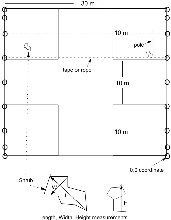
Equipment needed: GPS and metal detector for locating 30 x 30 m plot corner plates; tape measures; Pin flagging; 50 x 20 cm Daubenmire quadrats, robel poles, data recording supplies

Procedure: For each 30 x 30 m plot, find the corner plats and mark with pin flags. From each corner plate, measure 2.5 m into the plot in each direction (e.g. from SW corner, measure 2.5 m east and 2.5 m north) and place pin flag (red points). These 4 pin flags mark the corners of a 6 x 6 grid of points for daubenmire/robel pole measurements. Pace from one corner flag to another, placing a pin flag every ~5 m (blue points). Once the edges are flagged, fill in the rest of the grid with a pin flag every 5 m based on pacing (green points). Grids should be laid out quickly without need to roll out tapes.

(34)

Each grid is referenced by the pasture letter/number combination, and then by whether its in an exclosure (UU) or grazed plot (GG). Sites in GZTX study will have up to 5 treatments (GG, UU, GU, UG, R). Eg, 10SW-GG refers to the grid in pasture 10SW that is the grazed control plot paired to the exclosure.

At each grid point, we sample veg composition using a 50 x 20 cm quadrat centered over the point, with visual estimation of basal and canopy cover for each species plus basal cover of bare soil, litter, lichen and dung. The basal cover of plants plus bare/litt/lich/dung should sum to approximately 100.

The Daubenmire cover classes are as follows: T= Trace (<1%), 1 = 1-5%; 2 = 5-14%; 3 = 15-24%; 4 = 25-39%, 5 = 40-59%, 6 = 60-100%. The code for bare ground is BARE, litter is LITT, and lichen is LICH. Scat, including rabbit, pronghorn, and cow should be considered as part of the litter cover. We identify only one Astragalus/Oxytropus to species—the vine like one is ASGR (with thinner leaves and small purple flowers). All others are lumped under the code ASOX. The two Orabanche species are coded OROB.

The canopy cover may be less or more than 100% as much of the plot may be litter or bare ground or the canopy may be layered and each species overhanging in the plot must be recorded. Basal cover should

theoretically add to 100%, but because you are doing classes and not actual percentages the midpoint of the classes will only approximately add to 100%.

Unknowns should be labeled as forb, grass or shrub with the codes UNFB, UNGR, or UNSH. If an unknown is encountered several times it should be given a number or name, and identified at a later date, and the data sheets recoded with the correct four-letter species code. Daubenmire cover classes should be used for recording basal cover of each species rooted in the plot, bareground and litter, and canopy cover of each species.

At each location, we also sample veg structure using a robel pole with 1 cm increments, taking an observation on the pole in each of the 4 cardinal directions. We record both the number of intervals completely obscured by vegetation, and the highest interval with some kind of obstruction, with the pole constructed and sighting height and distance according to Robel (1970), but with the modification of using 1 cm increments. See the file ―‗Robel_Pole_Method_HighvsLow.ppt‖ for instructions on how to read the low and high values from the pole. In addition, record the species that is responsible for causing the obstruction associated with the

LOW reading; if more than one species is involved, record the tallest species associated with the LOW reading. Only one species code is recorded for each robel reading – there will be no species recorded in association with the HIGH reading. See example file.

(35)

Root Ingrowth Donut Procedure:

See the “Root Ingrowth Donut Protocol” below in this manual for sampling method details. Below is only the information concerning the numbers and locations of samples specific to GZTX.

There are two (2) root ingrowth donuts at each treatment within each site. Only the GZGZ and UNUN treatments are sampled and only five of the six sites (5 west, 5 east, 7, 11, 24 – 19 is not sampled for roots). Therefore, there are 5 sites X 2 treatments X 2 locations = 20 donuts. There are two depths sampled at this study (0-10 and 10-40cm), except that two of the donuts are not beveled and the 0-10cm depth must be cut without the PVC guide (bring a ruler with cm to measure this).

Use check-off sheet to account for all samples at end. Bag label example:

GZTX donuts Date (mo/day/yr)

Site (5 west, 5 east, 7, 11, 24) Treatment (GZGZ or UNUN) Plot (plot 1 or plot 2) Depth (0-10 or 10-40)

Bag number (1 of 2or3.., 2 of 2or3, …. QAQC Instructions for cover:

CAN OTHER PEOPLE UNDERSTAND YOUR WRITING???

IMPORTANT – Double check-off procedure (use the correct check-off sheet for that site and treatment). When starting a site-treatment, one person will be in charge of checking off plots on the master check-off sheet as the flags are inserted. As each team collects data from a plot they must pull the flag, unless it is a CLIP plot in the ungrazed treatments. The plot number should have a C, indicating CLIP, if the flag should stay. Each team will call the plots from where they have collected data to the person with the check-off sheet. The person with the check-off sheet and the team member will double check the plot numbers. The team member will make sure that this information is complete and correct on the data sheet. The person with the check-off sheet will double check

2011 field crew sampling protocols

SGS/LTER Field Staff & Research Assistants 2011

CSU SGS/LTER Field Station Address:

14791 Weld County Road 114

Nunn, Colorado 80648

SGS/LTER Field Research Staff

Site Manager: Mark Lindquist

(970) 897-2210,

mark.lindquist@colostate.edu

Field Crew Leader: Kevin Meierbachtol

Assistant Crew Leader: Trace Martyn

SGS/LTER Research Assistants

(May 16 to August 22)

Melissa Perkins

Brian Gley

Keith Porter

Amy Kousch

ARS

*For Emergency use

Site Manager: Mary Ashby

(970) 897-2226

Instructions for Hardwire Connections

1. Open your local area network settings as follows:

Click Start>Control Panel>Network Settings

Double Click Local Area Connections

2.

Click the General Tab and Double Click Internet Protocol (TCP/IP)

3. In the properties dialog click these options

Obtain an IP Address Automatically

Obtain DNS server automatically

Instructions for Wireless Connections

1. Open your wireless network settings as follows:

Click Start>Control Panel>Network Settings

Double Click Wireless Network Connections

2. Click View Wireless Networks

3. Double Click sgslter network box

ARS #03 Ecosystem Stress Area (ESA)

Principal Investigator:

Daniel.Milchunas@colostate.edu

North

T

4

T

3

T

2

T

1

T5

See map for D2

control and

grub kill plots

P

1

P1

0

T5,

P1-5

T5, P6-10

ARS Study #3 (ESA)

PI – Dan Milchunas

Recorder___________

Page ___of___

Data Entered By________

Date of Collection_____

Density

Sit

e

Da

ta Ty

pe

Mont

h

Ye

ar

Tr

ea

tm

ent

R

_{See map for D2}

Page _of_

_Tr

Page _of_

_Tr

_Basal

Date Recorder(s):___________________

Block:(E or W) Treatment:__(W, N, W+N, or C)

Transect:_(1, 2, or 3) Plot: ______(1, 2, 3, 4, 5, or 6) Dig Image