ADVANCING INTERNAL EROSION MONITORING USING SEISMIC METHODS IN FIELD AND
LABORATORY STUDIES
by Minal L. Parekh
© Minal L. Parekh 2016 All Rights Reserved
ii
A thesis submitted to the Faculty and the Board of Trustees of the Colorado School of Mines in partial fulfillment of the requirements for the degree of Doctor of Philosophy (Civil Engineering). Golden, Colorado Date ____________________________ Signed:____________________________ Minal L. Parekh Signed:____________________________ Dr. Michael A. Mooney Thesis Advisor Golden, Colorado Date ____________________________ Signed:____________________________ Dr. John McCray Department Head and Professor College of Engineering and Computational Science
iii ABSTRACT
This dissertation presents research involving laboratory and field investigation of passive and active methods for monitoring and assessing earthen embankment infrastructure such as dams and levees. Internal erosion occurs as soil particles in an earthen structure migrate to an exit point under seepage forces. This process is a primary failure mode for dams and levees. Current dam and levee monitoring practices are not able to identify early stages of internal erosion, and often the result is loss of structure utility and costly repairs. This research contributes to innovations for detection and monitoring by studying internal erosion and monitoring through field experiments, laboratory experiments, and social and political framing
The field research in this dissertation included two studies (2009 and 2012) of a full-scale earthen embankment at the IJkdijk in the Netherlands. In both of these tests, internal erosion occurred as evidenced by seepage followed by sand traces and boils, and in 2009, eventual failure. With the benefit of arrays of closely spaced piezometers, pore pressure trends indicated internal erosion near the initiation time. Temporally and spatially dense pore water pressure measurements detected two pore water pressure transitions characteristic to the development of internal erosion, even in piezometers located away from the backward erosion activity. At the first transition, the backward erosion caused anomalous pressure decrease in piezometers, even under constant or increasing upstream water level. At the second transition, measurements stabilized as backward erosion extended further upstream of the piezometers, as shown in the 2009 test. The transitions provide an indication of the temporal development and the spatial extent of backward erosion.
The 2012 IJkdijk test also included passive acoustic emissions (AE) monitoring. This study analyzed AE activity over the course of the 7-day test using a grid of geophones installed on the embankment surface. Analysis of root mean squared amplitude and AE threshold counts indicated activity focused at the toe in locations matching the sand boils. This analysis also compared the various detection methods employed at the 2012 test to discuss a timeline of detection related to observable behaviors of the structure.
The second area of research included designing and fabricating an instrumented laboratory apparatus for investigating active seismic wave propagation through soil samples. This dissertation includes a description of the rigid wall permeameter, instrumentation, control,
iv
and acquisitions systems along with descriptions of the custom-fabricated seismic sensors. A series of experiments (saturated sand, saturated sand with a known static anomaly placed near the center of the sample, and saturated sand with a diminishing anomaly near the center of the sample) indicated that shear wave velocity changes reflected changes in the state of stress of the soil. The mean effective stress was influenced by the applied vertical axial load, the frictional interaction between the soil and permeameter wall, and the degree of preloading. The frictional resistance was sizeable at the sidewall of the permeameter and decreased the mean effective stress with depth. This study also included flow tests to monitor changes in shear wave velocities as the internal erosion process started and developed. Shear wave velocity decreased at voids or lower density zones in the sample and increased as arching redistributes loads, though the two conditions compete.
Finally, the social and political contexts surrounding nondestructive inspection were considered. An analogous approach utilized by the aerospace industry was introduced: a case study comparing the path toward adopting nondestructive tools as standard practices in monitoring aircraft safety. Additional lessons for dam and levee safety management were discussed from a Science, Technology, Engineering, and Policy (STEP) perspective.
v
TABLE OF CONTENTS
ABSTRACT ... iii
LIST OF FIGURES ... viii
LIST OF TABLES ... xvi
LIST OF SYMBOLS AND ABBREVIATIONS ... xvii
ACKNOWLEDGMENTS ...xx
INTRODUCTION ...1
CHAPTER 1 1.1 Introduction and Motivation ... 1
1.2 Background: Knowns and Needs ... 3
1.2.1 Internal Erosion ... 3
1.2.2 Critical Vertical Exit Gradient-Effective Stress Approach ... 5
1.2.3 Laboratory and Numeric Characterization of Internal Erosion ... 5
1.2.4 Field Characterization of Internal Erosion ... 11
1.2.5 Geophysical Techniques ... 14
1.3 Social and Political Context for Research ... 17
1.4 Structure of dissertation ... 17
IJKDIJK INTERNAL EROSION EXPERIMENT: BACKWARD CHAPTER 2 EROSION MONITORED BY PORE PRESSURES ...20
2.1 Description of IJkdijk ... 20
2.2 Analysis of groundwater contours ... 30
2.3 PWP transitions characteristic of backward erosion ... 31
2.4 Conclusions ... 42
2.5 Acknowledgements ... 43
NON-DESTRUCTIVE ACOUSTIC EMISSIONS MONITORING AT CHAPTER 3 IJKDIJK ...44
3.1 Introduction ... 44
3.2 Baseline Characterization ... 45
3.2.1 Electrical resistivity, seismic refraction, self-potential ... 45
3.2.2 Terrestrial Remote Sensing ... 47
3.3 Acoustic Emissions ... 48
3.3.1 Test Details ... 48
3.3.2 AE RMS amplitude and counts... 52
vi
3.4.1 AE localization... 64
3.4.2 Passive seismic interferometry ... 64
3.4.3 Terrestrial Remote Sensing ... 64
3.4.4 Self-Potential... 65
3.4.5 Fiber Optic Temperature and Strain Monitoring ... 65
3.5 Discussion ... 66
3.5.1 Integration of all instrumentation... 67
LABORATORY PERMEAMETER APPARATUS AND ACTIVE CHAPTER 4 SEISMIC WAVE MEASUREMENT SYSTEM ...70
4.1 Rigid Wall Permeameter ... 70
4.2 Instrumentation ... 70
4.3 Compressional and Shear Wave Speed Measurements ... 74
4.4 Data Acquisition ... 78
4.5 Pressure and Flow System Control ... 80
LABORATORY TIME-LAPSE ACTIVE SEISMIC MONITORING OF CHAPTER 5 LOCALIZED EFFECTIVE STRESS CHANGES ...81
5.1 Test Summary ... 81
5.2 Specimen Placement ... 84
5.3 Baseline characterization of Vs velocities in saturated sand ... 86
5.4 Static Anomaly Testing... 96
5.5 Diminished Anomaly Testing ... 100
5.5.1 D4A: salt pellets ... 100
5.5.2 D5A: Water filled latex balloon ... 105
5.6 Vs Change During Flow ... 108
5.6.1 Flow test: F6 ... 110
5.6.2 Flow test: F7 ... 114
5.7 Conclusions ... 119
5.8 Recommendations for improvements ... 120
FROM RUNWAYS TO SPILLWAYS: A CASE STUDY FROM THE CHAPTER 6 AEROSPACE INDUSTRY ON ADOPTION OF NON-DESTRUCTIVE INSPECTION TOOLS WITH LESSONS FOR DAM SAFETY ...121
6.1 Abstract ... 121
vii
6.2.1 The need ... 123
6.2.2 Case study ... 124
6.3 Social and Political Framing ... 125
6.4 Evolution and Innovation of ND Technology and Policy in Aerospace 129 6.4.1 1950s-70s: Emergence of materials science and safety research (PROBLEM) ... 131
6.4.2 1980s: Materials Research (SOLUTION) ... 135
6.4.3 1990s: Agency partnerships (POLITICAL STRUCTURE) ... 135
6.4.4 2000s: Damage Tolerance Requirement (WIDESPREAD SOLUTION) ... 136
6.5 Evolution of policy in levees and dams ... 137
6.5.1 1960s-mid 1970s: Focus on Inspection and Cataloging (PROBLEM) ... 138
6.5.2 Late 1970s-1990s: Development of Federal Programming (POLITICAL STRUCTURE) ... 140
6.5.3 2000s: Attention on Levees and Risk-Based Decision Making (PROBLEM and POLITICAL STRUCTURE) ... 142
6.6 Contextual Comparison ... 143
6.6.1 Obstructions to the Comparison... 143
6.6.2 The Common Ground ... 145
6.7 Conclusion: Lessons and Recommendations ... 153
CONCLUSIONS AND RECOMMENDATIONS FOR FUTURE RESEARCH .156 CHAPTER 7 7.1 Field Experiments ... 156
7.2 Laboratory experiments ... 157
7.3 Science and technology innovation ... 159
REFERENCES CITED ...160
APPENDIX A GEOPHYSCIAL TECHNIQUES TO MONITOR EMBANKMENT DAM FILTER CRACKING AT THE LABORATORY SCALE ...171
APPENDIX B COORDINATING INTELLIGENT AND CONTINOUS PERFORMANCE MONITORING WITH DAM AND LEVEE SAFETY MANAGEMENT POLICY ...184
viii
LIST OF FIGURES
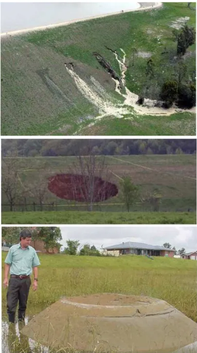
Fig. 1.1 Internal erosion through an embankment dam (top), sinkhole likely resulting from concentrated leak erosion below an embankment dam (middle) and sand
boil downstream of an earthen levee (bottom). ...2
Fig. 1.2 Cross section (top), elevation (middle), oblique photograph during testing (bottom) of Internal Erosion Embankment Testing, Norway (Hanson, 2007). ...12
Fig. 2.1 IJkdijk location in the northeast area of The Netherlands. ...21
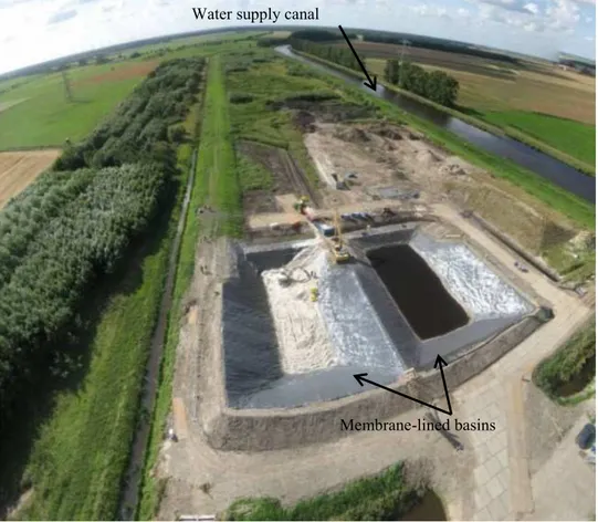
Fig. 2.2 Aerial view of IJdijk site during a typical test preparation. Two membrane-lined basins (before embankment placement), and water supply canal are shown. ...22
Fig. 2.3 View of upstream embankment slope (a) before reservoir raise, view of downstream embankment slope from right abutment (b) prior to instrument placement. ...26
Fig. 2.4 Foundation sand during compaction and placement of geotextile. ...27
Fig. 2.5 T2009 embankment and piezometer locations. ...27
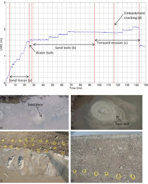
Fig. 2.6 T2009 loading and observations (van Beek et al. 2009) Wiring is visible in (c) and (d) as yellow circles but had minimal effect on the seepage and internal erosion process. ...28
Fig. 2.7 Foundation sand with vertical geotextile and fiber optics. ...29
Fig. 2.8 T2012 embankment and piezometer locations. ...29
Fig. 2.9 T2012 loading and visual observations. ...32
Fig. 2.10 Sand boils approximate locations and sand production for (a) T2009 and (b) T2012. For T2009, the plot qualitatively presents two stages of sand boil activity as different line thicknesses: 1) thin lines indicate the appearance of discrete sand traces or localized preferential flow, and 2) thicker lines indicate growing sand boils depositing sand material in a crater around a hole. For T2012, the plot provides a quantitative cumulative summary, with line thickness varying based on relative cumulative mass removed based on field measurements. ...33
ix
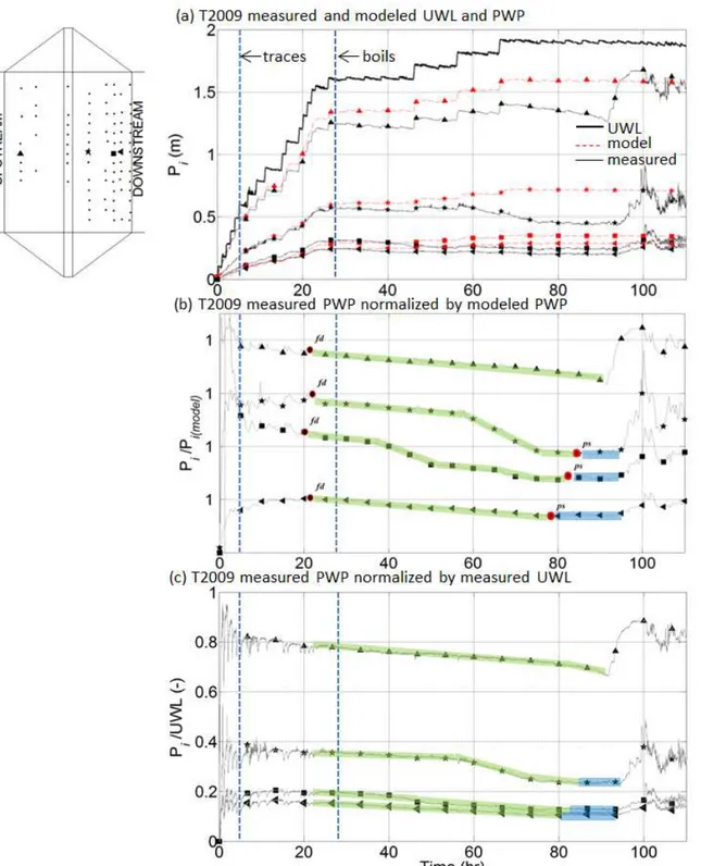
Fig. 2.12 T2009 select piezometer locations along a center transect showing (a) absolute PWP and modeled PWP, (b) PWP normalized by model results (Pi/Pi(model)), and (c) PWP normalized by UWL (Pi/UWL) for results truncated at 110 hrs.
Measurements and model results plotted ~every minute, but markers are shown at wider intervals purely for identifying piezometer location. ...36 Fig. 2.13 T2009 temporal transition points ps mapped over the shaded footprint (a). The
difference between fd and ps (b) provides an approximate time for internal erosion to propagate from the toe backwards to piezometer locations in the
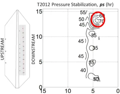
foundation. ...38 Fig. 2.14 T2012 piezometer locations along a center transect showing (a) absolute PWP
(Pi) and modeled PWP, (b) PWP normalized by model results (Pi/Pi(model)), and (c) PWP normalized by UWL (Pi/UWL) for test truncated at 110 hrs.
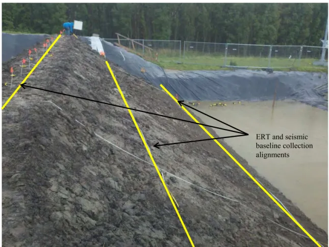
Measurements and model results plotted ~every minute, but markers are shown at wider intervals purely for identifying piezometer location. ...40 Fig. 2.15 T2012 temporal transition points ps mapped over the shaded footprint. ...41 Fig. 3.1 Baseline data collection alignments for both ERT and active seismic data
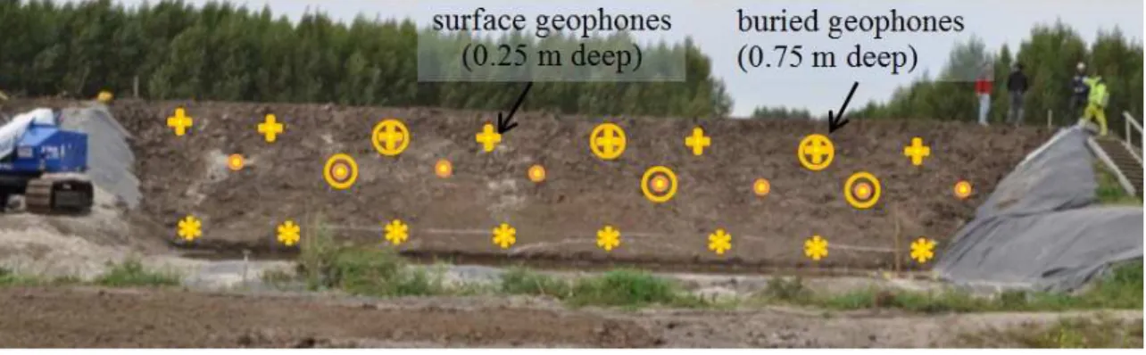
collection. ...47 Fig. 3.2 LIDAR (TLS) and radar (TRS) locations downstream of embankment. ...48 Fig. 3.3 Approximate locations of geophones embedded on downstream slope (elevation
view). Circled geophones were buried 0.75 m deep; the remaining were buried 0.25 m deep. ...49 Fig. 3.4 Plan view layout of geophones on downstream slope of embankment showing
channel numbering scheme. Circled geophones were buried 0.75 m deep; the
remainder 0.25 m deep. ...49 Fig. 3.5 Geophone before embedding. ...50 Fig. 3.6 Sum of all channels, raw (unfiltered) signals (a). Example single channel plots of
frequency content from row of geophones at toe to demonstrate variability in unfiltered frequency content in various channels (b). Geophone locations shown (left). ...51 Fig. 3.7 Average FFT of filtered signals from active and inactive time periods (10-min)
x
Fig. 3.8 Approximate locations of sand boils and sand production .The plot provides a quantitative cumulative summary, with line thickness varying based on relative
cumulative mass removed based on field measurements. ...53
Fig. 3.9 UWL (top) compared to total sand produced by sand boils and cumulative AE counts from all channels (bottom). ...54
Fig. 3.10 UWL (top) and total sand boil accumulation shown with three individual sand boils (bottom). The locations at the downstream toe for the three chosen sand boils are shown on the left in plan view. ...55
Fig. 3.11 UWL (top) and culmulative AE counts (threshold =10*RMS baseline) from all channels (bottom). CH8, CH9, and CH24 in transect the along left abutment are highighlighted ...57
Fig. 3.12 Normalized RMS amplitude for three channels as examples. ...58
Fig. 3.13 Normalized RMS amplitudes with time for all channels in three rows, windowed (15 min) moving maxima and minima shown in gray, average during nighttime plotted in red. ...59
Fig. 3.14 AE counts of peaks exceeding threshold =10 from three channels with nighttime measurements plotted in red. ...60
Fig. 3.15 AE counts exceeding threshold 10 (windowed moving average) plotted for all channels with time, with nighttime measurements plotted in red. ...62
Fig. 3.16 Spatial distribution of RMS amplitude (left column) and AE counts (right column) from 16-sec record at times shown (not cumulative). Cumulative sand production indicated by black circles at the toe of the embankment with diameter of circle proportional to mass of sand removed...63
Fig. 3.17 Annotated detection timeline integrating all monitoring and observations ...69
Fig. 4.1 Rigid wall permeameter installed in load frame. ...71
Fig. 4.2 Top view of bottom platen. ...71
Fig. 4.3 Experimental apparatus schematic (a) and physical arrangement (b) including: 1. Deaired water tank, 2. Upstream pressurized tank, 3. Rigid cell permeameter, 4. Downstream constant head tank. Pressure control panel shown in the photo was not used in these experiments. ...73
xi
Fig. 4.4 PP transducer mounting and spacing. ...75 Fig. 4.5 PP measurement locations. ...75 Fig. 4.6 Pore pressure measurements for air pressure set at top of water-filled
permeameter with PP sensors mounted in wall. For this calibration test, PPu and PPd were placed on the benchtop near the permeameter base. Sensor locations labeled (top) and line color (bottom) correlates to sensor location. ...76 Fig. 4.7 Load calibration verification between top and bottom load cells raw (a) and
linear relation (b) with 1:1 line plotted as reference. Steel spacers were used to transfer load between top and bottom. ...77 Fig. 4.8. P wave piezoelectric pad painted with insulating polyurethane (a), S wave bender
element painted with insulating polyurethane (b). ...79 Fig. 4.9 Typical piezoelectric sensor locations in permeameter without soil sample (a).
Sensors mounted on blocks (b) and placed within permeameter (c) as viewed
from above. ...79 Fig. 5.1 Typical seismic sensor locations in permeameter (shown without sand specimen).
Direct travel paths between aligned pairs (S1, S2, S3, S4) shown with scheme
used to describe sensor locations (color, line style, label). ...82 Fig. 5.2 Sand characteristics (Sakaki and Illangasekare 2007; Unamin Corporation 2007) ...83 Fig. 5.3 Top lift during flow testing showing clay cap and gravel leveling course below
top platen. ...86 Fig. 5.4 Baseline test N1. Axial vertical stress at specimen top and bottom (a) and top
plate ∆ and strain (b) Received waves shown with P arrival times (filled
circles) and S arrival times (diamonds) for sensor pairs 1 (c) and 4 (d). Values for ’v at sensor depths calculated based on the exponential interpolation between top and bottom load cell measurements. ...89 Fig. 5.5 Schematic of slice located at depth z between ’v,top and ’v,bottom for calculation
of ’v(z). ...90 Fig. 5.6 For test N1, ’v,top plotted with ’v,bottom (top plot) and ’v,top plotted with strain
(bottom plot) for load and unload. Neither ’v,bottom nor strain is fully recovered upon unload. ...92
xii
Fig. 5.7 Vs for various vertical axial loads applied at the top of the sample for baseline tests N1, N2 during load and unload. Vs is higher during the unload cycle,
reflecting a higher ’m at the sensor depths after preloading. ...94 Fig. 5.8 Vs for various vertical axial loads applied at the top of the sample for baseline
tests F6, F7 during load and unload. Vs is higher during the unload cycle,
reflecting a higher ’m at the sensor depths after preloading. ...95 Fig. 5.9 NI power fit rule relationship between Vs and �′ (Cha et al. 2014). ...97 Fig. 5.10 Power rule α(’m)β fit parameters α and β for four baseline tests (N1, N2, F6, F7)
at S1, S2, S3, S4 during loading and unloading. ...98 Fig. 5.11 N1 Vs calculated based on the relationship to �′ summarized in Ishihara (1996)
based on typical values for parameters A and n during load and unload. The
change in e as a result of preloading has minimal effect on Vs. ...99 Fig. 5.12 N3A Static anomaly (balloon) shown from side during specimen placement with
sensor pairs (a) and from top (b). Dimensions and balloon location with respect to sensors shown schematically. ...99 Fig. 5.13 Test N3A Vs at various vertical axial loads applied at the top of the sample. ...100 Fig. 5.14 N3A power fit during load and unload. ...101 Fig. 5.15 Power rule fit parameters for N3A (vertical limits of balloon denoted by green
horizontal lines). ...102 Fig. 5.16 D4A Salt pellets before placement (a). Salt anomaly shown in schematically in
relation to sensor locations (b) and in permeameter during placement, from above (c). ...103 Fig. 5.17 Test N4A Vs at various vertical axial loads applied at the top of the sample. ...105 Fig. 5.18 N4A power fit during load and unload. ...106 Fig. 5.19 D4A Power rule fit parameters (vertical limits of salt denoted by cyan horizontal
lines), t=0 hrs (before salt dissolution). ...107 Fig. 5.20 D4A test with salt anomaly. Constant ’v (275 kPa) applied during salt
xiii
dissolution period (b), change in Vs relative to start (c). Sensor pair at bottom
(S4) not shown because of sensor malfunction during dissolution. ...108
Fig. 5.21 Test D4A conceptual progression of f and stress conditions at start (a), during salt dissolution (b), and after all salt dissolves (c). ...109
Fig. 5.22 Test D5A Diminished balloon anomaly placement and schematic showing dimensions of balloon with respect to sensors. ...109
Fig. 5.23 Test N5A Vs at various vertical axial loads applied at the top of the sample. ...110
Fig. 5.24 N5A power fit load and unload. ...111
Fig. 5.25 D5A Power rule fit parameters (vertical limits of the balloon denoted by horizonal orange lines) ...112
Fig. 5.26 Test D5A as balloon loses volume from draining, strain (a), ’v,bottom (b), DL (b), ’m at sensor locations (c) and ∆Vs between sensor pairs (d). ...113
Fig. 5.27 F6 flow test with measurements PPu and PPd (a), iglobal (b), strain (c), D’m, and DVs (e) for the test duration. Gaps in PP and i indicate periods when valves where closed so that PPu and PPd were not applied to the sample. Dot markers on (d) and (e) indicate Vs aqcuisition times. ...115
Fig. 5.28 Piezometer locations and local ix during flow tests ...116
Fig. 5.29 F6 iglobal and local ilocal (smoothed over 30 sec) during F6 flow ...117
Fig. 5.30 Test F7 PPu and PPd (a), iglobal (b), strain (c), ∆�′ (d), and ∆Vs (e) during flow. Gaps in PWP and i indicate periods when external PP was not applied. ...118
Fig. 5.31 F7 iglobal and ilocal (smoothed over 30 sec). Gaps in i indicate periods when external PP was not applied. ...119
Fig. 6.1 Kingdon’s model for agenda setting ...127
Fig. 6.2 General timeline summarizing progress toward ND in aerospace. ...132
xiv
Fig. A.1 Laboratory layout of filter model showing: (a) assembled model, (b) upstream channel, (c) constant head reservoir, (d) uncracked filter, and (e) cracked filter (2.5 cm) ...174 Fig. A.2 Approximate CT raypath coverage between source (left edge) and receiver (right
edge) locations for T11 and T12 (boxes represent discretization for tomography modeling) ...175 Fig. A.3 Schematic (left) and pre-crack photograph (right) of filter geometry and
instrumentation for T11 – two stage filter ...177 Fig. A.4 Schematic (left) and post-crack photograph (right) of filter geometry and
instrumentation for T12 – single stage filter ...177 Fig. A.5 AE signatures during three stages of T12: Pre-cracking baseline (left), post filter
cracking during concentrated flow (center), and subsequent sidewall-collapse and self-healing events (right) ...180 Fig. A.6 Scatter plots of p-wave travel time versus source-receiver separation for T12
data. Trend lines have been added to depict the overall relative decrease in
calculated velocities over the course of T12. ...180 Fig. A.7 P-wave tomograms for T12 data collected pre-crack (left panel), and 2hrs and
24hrs after cracking of filter material and subjection to concentrated flow (center panel and right panel respectively) ...182 Fig. A.8 Plan view contour plots of electric potential distributions (SP data) at select
time-steps after initial cracking of filter material and subjection to fluid flow during T11. ...182 Fig B.1 Seismic sensors are connected directly to the mote circuitry. Other geophysical
sensors connect to the mote through the black waterproof connectors on the PVC casing (pictured on the right side of the mote enclosure in a)). The PVC
enclosure protects the geophysical mote circuitry from environmental harm. The PVC pipe does not affect performance of the network. The PVC piping protects the motes while allowing motes to collect geophysical measurements and
communicate wirelessly with other motes in the network to assess autonomously the integrity of the dam or levee. ...191 Fig B. 2 Conceptual representation of a WSN deployed at the surface of an embankment
and equipped to sense subsurface conditions. (a) WSN layout on an earthen zoned embankment dam with low permeability core. (b) Nodes are capable of communicating with all other nodes. Sensors interrogate node to node (only a few sample communications shown). Signals are “regular” under normal
xv
operating conditions. Black lines indicate regular signals. (c) At initiation of an anomalous event, signals indicate subsurface changes (such as internal erosion, as shown conceptually here.) Red lines indicate changing signals. (d) As the event continues, the subsurface features grows, WSN continues to detect
xvi
LIST OF TABLES
Table 1.1 Typical Values for Bligh’s E relationship ...6
Table 2.1 Sand Properties ...24
Table 4.1 Summary of Instrumentation ...72
Table 5.1 Testing Summary ...83
Table 5.2 Test Details ...84
Table 5.3 Top and bottom effective stress summary (applied load shown in parentheses) ...87
Table 5.4 Summary of baseline testing after loading ...91
Table 5.5 ∆�′, preload summary ...91
Table 6.1 Noteworthy events and organizational developments in the aerospace industry toward innovation of nondestructive tools ...130
Table 6.2 Noteworthy events and organizational developments in the dam and levee industry ...139
xvii
LIST OF SYMBOLS AND ABBREVIATIONS
AE ... acoustic emissions
AFRL ... Air Force Research Laboratory
ASDSO ... American Society of Dam Safety Officials ASIP ... Air Structural Integrity Program
� ... angle of internal friction E ... Bligh's empirical relationship
... coefficient of friction between specimen and permeameter wall
Cu... coefficient of uniformity
Vp ... compressional (P) wave velocity ic ... critical vertical gradient
Hc ... critical head
∆L ... deformation, change in height of specimen SP ... electrical self-potential
FAA... Federal Aviation Administration
FEMA ... Federal Emergency Management Agency FERC... Federal Energy Regulatory Commission fd ... first detection PWP decrease
Q ... flow rate f ... friction
F ... frictional side resistance force iglobal ... global hydraulic gradient HET ... Hole Erosion Test K ... hydraulic conductivity H ... hydraulic head
ICOLD ... International Committee on Large Dams
ib ... local hydraulic gradient at the bottom of specimen it ... local hydraulic gradient at the top of specimen ix ... local hydraulic gradient at sensor x
xviii L ... length
LST ... Levee Screening Tool LIDAR ... light detection and ranging
... mass density
�′ ... mean effective stress
NASA ... National Aeronautics and Space Administration NCLS ... National Committee on Levee Safety
NDSP ... National Dam Safety Program
NIST ... National Institute of Standards and Technology NID ... National Inventory of Dams
NLD ... National Levee Database
NMAB... National Material Advisory Board ND ... non-destructive
NDE ... non-destructive evaluation NDI ... non-destructive inspection PP ... pore pressure
PPd ... pore pressure downstream PPi ... pore pressure at transducer i PPu ... pore pressure upstream PWP ... pore water pressure ps ... pressure stabilization Dr ... relative density
R&D ... Research and Development RMS ... Root Mean Square
Vs ... shear (S) wave velocity Gs ... specific gravity
∆L/L ... strain
TLS ... terrestrial LIDAR scanning � ... total vertical stress
USCS... Unified Soil Classification System ... unit weight of soil particles
xix
′ ... unit weight of soil, buoyant ... unit weight of water
USAF ... United States Air Force
USACE ... United States Army Corps of Engineers USBR ... United States Bureau of Reclamation USDA ... United States Department of Agriculture UWL ... upstream water level
�′ ... vertical effective stress
�′ , ... vertical effective stress at the specimen top
�′ , ... vertical effective stress at the specimen bottom
e ... void ratio
WRDA ... Water Resources Development Act ... White's constant
xx
ACKNOWLEDGMENTS
It takes a village to raise any student, no matter her age. I express sincere gratitude to the village that supported me as I pursued my degree. I thank my advisor, Mike Mooney, for selling the idea of the PhD to me and leading me through the process, always with humor. I thank Jason Delborne and Jennifer Schneider, my STEP minor advisors, for guiding me to look at my
profession through a new lens and for laughing at my inappropriate jokes. I thank the entire SmartGeo research group, especially Ben Lowry, Nathan Toohey, Kerri Stone, Scott Ikard, Bryan Walter, Carolyne Bocovich, Thomas Planes, Wim Kanning and Minsu Cha. These kind and generous colleagues supported my professional and personal growth through their intellect, friendship and creativity. I thank the National Science Foundation, HydroReserach Foundation and USACE RMC for funding my work. Last but far from least, I thank my family near and far, most especially my husband, Bo, and our two children, Angela and Sakeia. They inspire me to open my mind, to work my hardest, to reach beyond my comfort zone, to ask important
questions and to seek meaningful answers. Together we learn patience and perseverance. I hope to give back to you all the grace you share with me.
1 CHAPTER 1 INTRODUCTION
1.1 Introduction and Motivation
Earth levees and dams provide flood protection, clean water supply and renewable energy for millions of people around the globe. In the US, most of these structures are approaching or operating beyond their design life. For example; according to the American Society of Civil Engineers (ASCE 2009), 85% of all dams in the US will have exceeded their 50 year design life by 2020 so continued reliable performance is a concern. In addition to addressing structural health because of aging, of equal importance is assessing existing dams for deficiencies in comparison to modern design and construction practices (Foster et al. 2002). The need to develop the science and tools for monitoring early stages of failure within the structures is critical so that intervention can prevent catastrophic damage and costly repairs.
Internal erosion is one of the primary processes threatening the structural health of earthen embankments, but observing the process beneath the surface is difficult. Schmertmann (2000) quotes the Building Research Establishment as saying “internal erosion can be a major threat to the safety of embankment dams, yet the mechanisms involved are not well
understood… The problem sometimes receives relatively little attention yet it may be the greatest hazard to the safety of many embankment dams.” Internal erosion typically is not recognizable until it becomes observable during visual inspections of the surface of an
embankment. Review of dam incidents and failures shows the first observable signs of erosion tend to be at progression (Fell et al. 2003), when a connection between the upstream and the downstream has already developed. Fig. 1.1 shows a few examples of internal erosion manifested at the surface of an earthen dam in the form of erosion channels, a sinkhole and a sand boil. By the time the process has reached this point, mitigation measures may be urgent at a high cost with few options for investigation and remediation.
The observational method is a key component of successful geotechnical engineering and performance of the geotechnical components of infrastructure. In his Ninth Rankine Lecture, Ralph Peck (1969), a pioneer in the field of soil mechanics, referenced Karl Terzaghi’s understanding of internal erosion and dam foundations in general: “Here the unavoidable
2
shortcomings in the knowledge of the subsurface conditions and their influence on the pore water pressures drew his [Terzaghi’s] attention to the necessity for a substantial element of empiricism in design.” Peck quoted Terzaghi: “Many variables, such as the degree of continuity of important strata or the pressure conditions in the water contained in the soils, remain unknown.”
Fig. 1.1 Internal erosion through an embankment dam (top), sinkhole likely resulting from concentrated leak erosion below an embankment dam (middle) and sand boil downstream of an earthen levee (bottom).
3
Peck summarized one of Terzaghi’s conceptualizations of the observational method: “Base design on information that can be secured. Make a detailed inventory of all the possible differences between reality and the assumptions. Then compute, on the basis of the original assumptions, various quantities that can be measured in the field…On the basis of such measurements, gradually close the gaps in knowledge and, if necessary, modify the design during construction….practical application of this “learn as you go” method” (Peck 1969).
The observational method extends beyond the design and construction phases for dams and levees. The structures are observed, inspected and evaluated throughout their service life as part of operation, maintenance, and safety programs. This dissertation addresses the challenge of detecting and identifying early stages of internal erosion in existing earthen embankments (specifically, dams and levees) using nondestructive (ND) techniques as part of applying the ongoing observational method well after design and construction. These studies focus on seismic and acoustic methods as early detectors, including evaluation of the chronological relationship between indicators such as direct observations of the dam/levee surface, geotechnical
instrumentation, electrical self-potential (SP), and remote sensing (LIDAR). To explore the potential for widespread application of new ND tools to the field, research also addresses the social and political context of this technical work.
1.2 Background: Knowns and Needs
This section presents the current state-of-the-art understanding of the internal erosion process and the use of ND tools. Published research includes little, if any, literature on early detection, or in-situ identification of initiation and continuation of internal erosion processes. The following sections define the internal erosion process, present analytic and numeric models for representing the mechanics of the process, describe previous field studies of internal erosion, and discuss the basis of geophysical techniques.
1.2.1 Internal Erosion
Inevitably, water flows or seeps through levees and earth dams. Internal erosion results when seepage transports soil particles to an exit point. The process can occur in the embankment, through the foundation and from the embankment into the foundation. Internal erosion initiates when an embankment experiences a critical combination of hydraulic gradient, in-situ stress conditions, soil porosity and intrinsic permeability. If internal erosion goes unchecked, meaning control of hydraulic loading and/or internal filters do not arrest the process, piping occurs and
4
can result in breach of a dam or levee. The four conditions that must exist for internal erosion to occur include:
1. the presence of a seepage path subjected to focused water flow;
2. the presence of erodible material, which can be carried by seepage flow within the flow path;
3. the presence of an exit point where eroded material can escape;
4. the ability for the material directly above a formed erosion zone or "pipe" to form and support a crown for the pipe or sustain an open crack (Mattson et al. 2008).
Mechanisms for initiation of internal erosion are categorized as suffusion, backward erosion piping, contact erosion, and concentrated leak erosion (Fell and Fry 2007). Internal erosion usually involves more than one of these mechanisms working in concert. Suffusion occurs when fine particles move through pore space of a coarser skeleton. Coarse graded and gap graded soils are susceptible to suffusion, where the volume of fines is less than the volume of voids between the coarse particles. Backward erosion piping occurs where cohesionless soils are subject to seepage uplift pressures that cause the soils to float or heave at the downstream
seepage exit point. Backward erosion piping commonly appears as a sand boil. The detached particles are carried away by the seepage flow and the process back-propagates until forming a continuous path (“pipe”) to the upstream reservoir. Soil contact erosion occurs where filter incompatibility exists at the interface between a material with fine particles and a coarse
material, for instance along the contact between silt and gravel, such that flow through the more permeable material erodes the adjacent material. Concentrated leak erosion occurs where cracks caused by differential settlement, desiccation, freezing and thawing, form in an embankment or its foundation. The concentrated flow at these cracks causes particle removal (“erosion” or “scour”) from the walls of the crack.
The stages of internal erosion are commonly characterized using four stages: 1. Initiation, when particles begin to move with seepage flow;
2. Continuation, when erosion may halt as seepage forces are reduced or passage of particles is impeded, i.e. as a result of material types, where filter transitions prohibit movement of material;
5
3. Progression, when a continuous flow channel forms as an open crack or other piping pathway. Visual indicators at the surface of a structure usually become apparent during the progression stage; and
4. Breach/failure, when sudden, rapid, uncontrolled flow is released from the reservoir as the embankment “breaks” (Fell and Fry 2007).
1.2.2 Critical Vertical Exit Gradient-Effective Stress Approach
The classic approach to describe the initiation of internal erosion includes analysis of the effective stress at the seepage exit. If the upward seepage forces on a body of soil exceed the gravitational forces at the point of exit, the vertical critical gradient (ic) is exceeded and soil particles may be removed from this area (Terzaghi et al. 1996). This phenomenon, called a quick condition, heave, or flotation, can cause removal of soil particles with moving water. The
approach is dependent on the specific gravity and density of the soil particles and is defined as:
� = ′ == +− (1.1)
Where ′ is buoyant unit weight of soil, is the unit weight of water, ic is dependent on specific gravity of solids (Gs) and void ratio (e). For typical values of Gs , and e for sand, ic is approximately 1. This method assesses whether particle movement will initiate at the
downstream exit but does not evaluate gradients required for piping to progress.
1.2.3 Laboratory and Numeric Characterization of Internal Erosion
Others researchers are working to characterize the physical mechanisms associated with the various internal erosion processes for the purpose of predicting conditions under which erosion will initiate and continue. For backward erosion, research has focused on developing empirical relations and experimental and numeric models to determine critical gradient or head at which the process initiates and continues to piping (van Beek et al. 2010; Koenders and Sellmeijer 1992; Lopez de la Cruz et al. 2011; Richards and Reddy 2007; Schmertmann 2000). For suffusion, previous research investigated factors affecting the initiation movement of fine particles through a coarse matrix (Benamar et al. 2010; Bendahmane et al. 2008; Bonelli et al. 2006; Fannin and Moffat 2008; Indraratna et al. 2011; Li and Fannin 2008; Moffat et al. 2011; Skempton and Brogan 1994; Wan and Fell 2004). Finally, for concentrated leak erosion, research
6
explored materials’ susceptibility to erosion in the presence of a crack or a channel (Bonelli et al. 2006; Hanson et al. 2010). These studies provide a basis for experimental investigation of
internal erosion, which is the focus of this dissertation.
1.2.3.1 Backward erosion
Richards and Reddy (2007) summarized work performed by W.G. Bligh in 1910 as the foundation for much of the modeling of the backward erosion process. Bligh related the length of flow to the tractive forces acting on particles. Using case study information from field failures, Bligh proposed a relationship:
= (1.2)
Bligh’s theory was termed the “line-of-creep theory”, derived to evaluate the piping potential along a contact between structures and soils (Richards and Reddy 2007). This
relationship assumed the seepage path is concentrated near the base of the earthen embankment, with L the length of the base of an embankment (levee) in cross section with the seepage flow and Hc is critical head, horizontally oriented. The ratio E was given as “rules of thumb” as shown in Table 1.1 (Ojha et al. 2003).
According to Robbins and van Beek (2015), E.W. Lane reviewed 278 dams to evaluate the creep ratios based on empirical data. Lane reduced the seepage length in Equation (1.2) by one-third to account for the increased resistance to flow provided by vertical barriers. However, Lane’s revision did not address the relative factor of safety against backward erosion piping (Robbins and van Beek 2015).
Table 1.1 Typical Values for Bligh’s E relationship
Foundation Material E
Riverbeds of light sandy sand 18
Fine micaceous sand 15
Coarse-grained sand 12
Boulders, gravel and sand 6-9
Sellmeijer (1988) derived the first analytical model to describe the backward erosion piping process controlled by sediment transport conditions at the bottom of the pipe, with steady
7
and viscous flow. This model was based on equilibrium of forces between sand grains and flow, shown in Equation (1.3) and Equation (1.4).
= ( ) tan θ − . . (1.3)
Where
= .
⁄ (1.4)
H is the difference in water height, L is length of structure, η is White’s constant for drag coefficient, d is diameter of particles, K is intrinsic permeability, is particle unit weight, is angle of friction for single particle stability. Sellmeijer defined a maximum head for which the sand grains are in equilibrium as the critical head, Hc. This model indicated that the growth of the
channel stops at a certain length if Hc is not exceeded. At critical head, the growth of the channel
will continue until the hydraulic head is lowered (van Beek et al. 2010). Sellmeijer’s model took the approach that not all sand boils represent critical conditions. The model has become the design standard in the Netherlands, but the model is sensitive to grain size and permeability (Robbins and van Beek 2015).
Schmertmann (2000) presented an empirically based design method for determining the factor of safety against internal erosion in cohesionless soils. This work suggested a strong dependence of the piping gradient on grain size, quantified using Cu, the uniformity coefficient (d60/d10) and the d70. The minimum gradient required for piping increased at a rate proportionally greater than the increase in Cu. This method was based on point gradients, defined as the local gradient upstream of an advancing pipe feature.
In general, for backward erosion piping, after initiation as the piping progresses, most of the head loss occurs at the upstream portion from the pipe tip because the head needed to initiate the piping is more than the head needed to carry away the sand particles that slide into the pipe. When self-healing occurs, the head loss is almost constant along the sample. The piping channel does not advance in a downstream to upstream straight line but instead meanders in a braided system of channels. Paths clog and progress halts until another path starts elsewhere (Redlinger 2013).
8
The increased horizontal and new vertical gradients loosen the soil at the pipe head sufficiently that the particles at the pipe head move downstream by some combination of rolling and sliding, driven by the viscous drag of the water flowing in the pipe and helped by the suspending action of the vertical gradients. The loss of particles at the pipe head causes the pipe to advance upstream, producing a new flow and gradient concentration at the pipe head.
Eventually, either the dam breaches because of rapid scour when the pipe reaches the upstream head source, or the pipe advance stops within the dam or its foundation because of insufficient gradient to continue the process (Redlinger 2013).
1.2.3.2 Suffusion/Suffosion
Skempton and Brogan (1994) performed piping experiments in unstable gravelly sands, or gap-graded sands to study suffusion. These studies showed hydraulic gradient at erosion failure is governed by effective stresses on the fine fraction. Critical gradient for suffusion was defined in terms of overall porosity and specific gravity of the particles. Matrix-supported materials may not pipe until ic, but still may lose fines. A successful filter needs to retain fines. Generally, materials with Cu <10 were considered self-filtering and Cu >20 were considered potentially unstable. The study concluded that in unstable sandy gravels, piping of sand can occur at hydraulic gradients 1/3 to 1/5 of the theorized critical gradient, less than the theorized piping gradient of homogenous sand.
Garner and Sobkowicz (2002) studied unstable gap-graded materials, such as occurs in glacial deposits, in a large-scale permeameter laboratory assembly. The testing first focused on determining whether hydraulic gradients could generate suffusion (defined in the paper as “redistribution of fines within a stable densely packed skeleton.”) or suffosion (defined in the paper as “mass movement of the fine fraction within the skeleton of a potentially unstable coarse fraction”.) Large concentrated gradients became apparent in the base material layer upstream of the interface between the base and filter materials, with local gradients as high as 243, when the overall average gradient across the sample was 37. The permeability in that layer reduced from 1.5 x 10⁻³ cm/sec to 1.75 x 10⁻⁶ cm/sec, explained as suffusion where fines migrated to that layer and became trapped. The existence of that “clogged” layer, the interface between base and filter materials was not subjected to high local gradients and fines migration at the interface was not realized. The largest gradient at the interface never exceeded 1.6.
9
Moffat and Fannin (2006) developed a rigid, transparent test permeameter to investigate the relation between effective stress in a soil and hydraulic gradient at the onset of suffusive failure. The permeameter subjected a sample to unidirectional flow while maintaining constant effective stress. A series of pressure transducers monitored spatial and temporal changes within the soil sample characterize the development suffusion and piping. Variables in the experiment included soil type (0 to 30 percent fines), vertical effective stress, average hydraulic gradient, and direction of flow (Moffat 2005; Moffat et al. 2011; Moffat and Fannin 2006). Movement of the fines as suffusion (as evidenced visually) occurred in tests subjected to downward flow, either as uniform loss or as preferential loss from discrete locations. The loss occurred as a time dependent condition shown by changes in localized hydraulic gradient in silty soils. Suffusion occurred as a transient condition, with the onset accompanied by an increase in hydraulic gradient. The rate of suffusion diminished as time elapsed. Particle movement (as suffusion) occurred in a distinctly preferred area in the final stage of tests. Visual observation revealed development of voids within the specimen, with voids periodically collapsing or in-filling with smaller particles. The location of preferred seepage varied with time. With upward seepage, fines migrated without constraint by the primary soil fabric, and the motion was accompanied by downward displacement of the top loading plate that sometimes generated an audible sound. Variation of local hydraulic gradient showed that the particle loss results in large and rapid change in local permeability and specimen volume change.
Moffat and Fannin (2011) also described the relationship between hydraulic gradient and stability index. While the study was specific to the core and transition zones of the WAC Bennett Dam in Canada, the study found that local decreases in hydraulic gradient within a test specimen were useful to interpret the start of internal instability—instability was defined by a temporally compressed decrease in local gradient. Spatial variation of localized hydraulic gradient and vertical effective stress were the key factors determining the location of instability within a specimen, with internal instability triggered either by an increase in hydraulic gradient or by a decrease in effective stress.
Bendahmane et al. (2008) developed an experimental device to apply hydraulic stresses to soils to study the erosion evolution and found a gain in the suffusion rate with increased hydraulic gradient and with reduced confining stress. The studies focused on remolded
10
fraction was a result of the suffusive process. With higher hydraulic gradient, the sand fraction eroded as backward erosion and the extent was governed by clay content. Confinement stress affected both erosion mechanisms. To define initiation of backward erosion, Bendahmane et al. related critical hydraulic gradient to hydraulic shear stress and intrinsic permeability.
Permeability decreased by factor of 10 when suffusion erosion initiated, indicating clogging. The erosion rate decreased linearly according to the confining pressure for given hydraulic gradient values because the higher the consolidation, the higher the contact bonds, so the higher the erosion resistance. Suffusion erosion of the clay fraction did not affect the overall particle size distribution or volume of sample, but did decrease the overall permeability.
The study by Bendahmane et al. also defined a secondary threshold value for gradient when sand particle migration initiates as backward erosion in a clay-sand mix, resulting in sample collapse. This second gradient depended on confining pressure and clay content, and typically is very high. For clay content over 10 percent, backward erosion was not observed in these tests. In contrast to suffusion, increased confinement showed “intensified” backward erosion, with erosion initiating at lower gradients.
Continuum-based models describing the suffusive internal erosion process as flow
through porous media were based on multi-phase approaches, in which the erosion is modeled by considering the mass exchange between the liquid-filled pores (suspension of fines in fluid) and the soil skeleton (solid). Steeb et al. (2007) discussed a multiphase model that addresses
fluidization and transport of fine material in a saturated granular matrix. The modeling framework described various aspects of suffusion erosion that results in a mixture of four constituents: the stable solid skeleton, the erodible (unstable) fines, the eroded particles, and the pore fluid. That research proposed constitutive equations that are strongly coupled and nonlinear.
Bonelli and Marot (2008) also looked at suffusion as bulk erosion, where in a clayey sand erosion occurred at the clay/water interface. A coefficient of surface erosion of the clay matrix quantified suffusion rate. These models framed internal erosion in continuum mixture theory and modelled a smooth transition from soil to fluid. The transition was described in three phases— solid, fluid, and fluidized—and has been applied to granular soils. This modeling of suffusion indicated that the macroscopic bulk erosion was driven by the pressure gradient and not by the seepage velocity.
11
1.2.3.3 Concentrated Leak
Erosion in flaws is not described by a flow net, but is due to flow in open cracks (Fell 2007). Small-scale bench top laboratory tests, such as the Hole Erosion Test (HET), quantified the erodibility of soils subject to concentrated leaks in laboratory settings. HETs have been used to quantify the rate of piping erosion in soils and for determining the critical shear stress
corresponding to the start of piping erosion. Soil erodibility, or enlargement of a flow path, has been described using an excess stress equation (Hanson et al. 2010). The HET was performed by starting flow through a predrilled hole at a low hydraulic head, typically 50 mm of water, and holding hydraulic head steady for as long as possible (up to 45 minutes) once erosion was observed. The test continuously monitored flow rates, hydraulic gradients, and records the initial and final hole diameters. As the hole diameter increased under constant head, the shear stresses increased, and the flow rate increased. The rate of erosion plotted against the computed shear stress during the progressive erosion graphically showed the coefficient of soil erosion and the critical shear stress (Wahl 2008).The relationship was expressed as the rate of erosion in terms of volume per unit area per unit time, or mass per unit area per unit time (Hanson et al. 2010).
The HET mostly has been used to evaluate the rate of erosion and critical shear strength of soils. The erosion rate index of a soil is influenced by degree of compaction and moisture content. A specimen at high dry density, compacted wet of optimum moisture content has a higher erosion index than the same material compacted at lower dry density and dry of optimum moisture content (Wan and Fell 2004). The critical shear strength of soil cannot be accurately estimated using HET. HET can be used to estimate resistance against initiation of erosion by identifying minimum test head below which erosion does not occur, with erosion occurrence defined by increased flow through the specimen.
1.2.4 Field Characterization of Internal Erosion
A few larger scale earth dam and levee tests have been constructed both in the laboratory (indoors) and in the field. The majority of embankment models examined failure caused by water flowing over the top of the dam (overtopping). Few studies focused on internal erosion processes (Hanson and Temple 2007; Wahl et al. 2008).
Physical models measuring 4.5 m to 6 m high by 36 m long were constructed in Norway to study overtopping in a zoned embankment rockfill with a glacial moraine core embankment, and in a homogenous marine clay embankment. An example from the study is shown in Fig. 1.2.
12
Fig. 1.2 Cross section (top), elevation (middle), oblique photograph during testing (bottom) of Internal Erosion Embankment Testing, Norway (Hanson, 2007).
These studies included two internal erosion experiments using an embedded pipe fitted with openings to start the erosion process. The time and volume of flow release and the size of the breach in the embankment was measured as failure progressed.
The IJkdijk test facility (pronounced “Ike dike”, meaning “calibration levee” in Dutch) was a project in the Netherlands where researchers performed large-scale experiments on full-scale constructed levees starting in 2009 (IJkdijk 2009). The first experiments involved a homogenous sand levee measuring 4 m high, 40 m long and 25 m wide. Monitoring included measuring water pressure and the deformation of the levee, and heat-sensitive cameras recorded the piping process. Fiber optics installed at the interface measured temperature and strain (van Beek et al. 2010; de Vries et al. 2010). Elevated water levels on the upstream side of the levee induced piping in the sand layer.
IJkdijk experiments determined temperature to be effective for detecting signs of failure by piping, especially during the progression phase. Fiber optics measuring both strain and
13
temperature predicted seepage/erosion, with better predictions for leaks closer to the fiber optic cables. Cables placed in sand provided better information than those in clay (de Vries et al. 2010).
Van Beek et al. (2010) described four phases observed in the full-scale field testing: seepage, retrograde erosion, widening of the channel and failure of the embankment. This work studied backward erosion compared to Sellmeijer’s model and concluded that channel formation occurred as sand traces (sandy spots without a sand-producing crater) and sand craters on the downstream toe. Sand traces appeared in the testing at a hydraulic head below the critical head predicted by the model. Sand-transporting craters appeared in the testing near the critical head. Pore pressure transducer measurements indicated the widening phase of the piping channel with a local drop in pore pressure (van Beek et al. 2010). These 2009 IJkdijk experiments were precursory to a 2012 experiment during which monitoring included not only densely spaced piezometers, but also geophysics and remote sensing discussed in this dissertation.
Understanding observable or measurable indicators in relation to the temporal
development of internal erosion, including length of erosion channels, is critical for predicting behavior and for determining intervention strategies. However, the time dependent relationship between observation of sand boils and breach is uncertain. A review of dam incidents and failures showed the first observable signs of internal erosion tend to be at progression, marked by localized concentrated flow and transported soil, and the time to breach may be hours to weeks (or even years) depending on soil characteristics (Foster et al. 2000; Fell et al. 2003). For levees, sand boils may indicate local heave initiated at much lower head (difference between upstream and downstream water levels) than required for progression, meaning the process self-arrests at the localized boil (van Beek et al. 2014). In this case, the presence of sand boils may not lead to breach. The IJdijk field testing was used to validate numerical modeling based on inter-granular forces in sand, flow in an eroding channel, and flow in the aquifer, related erosion channel length to head at which sands are in equilibrium (van Beek et al. 2010; Sellmeijer et al. 2011). Sellmeijer’s model as discussed above predicted critical horizontal gradient (defined as horizontal gradient, head difference divided by length of the seepage path, across structure) and was a function of the aquifer properties (e.g. thickness) and material properties (e.g. grain size, hydraulic conductivity).
14
1.2.5 Geophysical Techniques
This research proposes to investigate two geophysical methods: 1) passive acoustic emission (AE) monitoring and 2) active seismic monitoring to identify time-dependent changes indicative of stress changes such as caused by a density anomaly or internal erosion. The following sections describe how these geophysical techniques successfully have characterized known areas of concern for dams and levees by identifying seepage or subsurface voids. However, they have not been used yet for spatially continuous, time-lapse monitoring for early detection of internal erosion.
1.2.5.1 AE in Soils
AEs are mechanical waves produced by deformation in a stressed material. AE
monitoring provides a means to passively monitor for concentrated seepage and internal erosion by using transducers (e.g., geophones or accelerometers) to sense (“listen for”) vibrations from acoustic energy released from internal sources including erosion and collapse events (Indraratna et al. 2011). In geologic materials, the source can be macro dislocations or grain boundary movements. Of all the non-destructive testing techniques, acoustic emission is unique, as the elastic waves are produced within the source material because of an external stimulus (change in pressure, strain, temperature) unrelated to the acoustic emissions acquisition procedure. Because collection of acoustic emissions data acquisition does not itself affect the material during
interrogation, the method is considered minimally invasive and non-destructive.
Acoustic emissions depend on the properties of the soil through which the waves travel, as well as the surrounding materials. The fundamental frequency character depends on source and distance between source and sensor. Frequencies less than 1 Hz have been observed at large field sites, while in laboratory studies frequencies greater than 500 kHz have been observed (Hardy 2003). Detection of an event by monitoring for acoustic signals depends on source spectrum, degree of and frequency dependence of attenuation, distance from sensor to source, and bandwidth and sensitivity of monitoring sensors. If the distance between the source and the sensor is large, then only low frequency components will be observed. If the spectrum of the source’s signal has no low frequency components, then this limit defines the critical range beyond which events are undetectable.
Koerner et al. (1976, 1977, 1978, 1979, 1981b) performed a series of fundamental studies in the 1970’s and 1980’s showing that deformation and seepage are sources of AE. That research
15
studied AE activity in soils in laboratory tests and in full-scale field tests. The early research addressed questions concerning the nature of the signal strength of the AE in soil during loading, the frequency content, and the attenuation while propagating through soil. Laboratory studies in granular soil yielded AE frequencies ranging from 500 Hz to 2 kHz during unconfined
compressive strength tests on dry silty sands (triaxial creep tests). Studies in cohesive soils showed signal amplitudes are 100 times stronger at failure than during early stress increments. Predominant frequencies were in the 2 kHz to 3 kHz range for clay samples tested in unconfined compression. Signals from a clay soil were half to 1/400 the levels from granular soils subject to the same stress level. The signal amplitude increased with increased stress, but stabilized and decreased before maximum stress is applied, a trend that Koerner explained as particle
reorientation. The overall number of emissions in granular soils significantly exceeded those in cohesive soils.
The studies continued with AE monitoring of seepage in field earthen embankments (Koerner et al. 1978). The field installations included downhole waveguides with accelerometers mounted on the ground surface. Attenuation rates in the waveguides (steel rods) were generally at least three orders of magnitude less than in soils. The field acoustic monitoring system included a piezoelectric accelerometer with a relatively flat frequency response from 500 Hz to 5,000 Hz at resonant frequency of 5,700 Hz. The system was deployed initially at 17 sites, then extended to include 11 additional sites (Koerner et al. 1981b). Based on this instrumentation, the researchers concluded that over 500 counts/min indicate an active instability mode, with AE activity increasing as seepage rate increases. AE activity also rapidly increased during rainfall events.
Koerner (1981a) continued the series of research regarding acoustic emission monitoring of soil stability by evaluating the technical feasibility of applying AE to monitor water seepage through soil. Acoustic emission rates from clear water and turbid water passing through a column of soil at various velocities were compared to a field leakage study. The parallel set of tests using turbid water indicates that, for equivalent flow rates, turbid water flow results in higher acoustic emission rates. The minimum detectable flow for turbid water is 10 ml/s.
Buck and Watters (1986) studied the influence of flow rate and soil type on AE. Those studies concluded that movement of the grains was likely required for AE emission, and
16
size, and 0.8 cm/sec in coarse sands with 0.2 mm to 0.8 mm effective size. The study counted number of events exceeding a voltage threshold to define AE activity.
Hung et al. (2009) studied AE in granular soils subjected to seepage in a laboratory experiment, showing that the spectral level for a specimen increased as seepage velocity increases. DiCarlo et al. (2003) showed that small hydro-mechanical disturbances in soils subjected to flow produced acoustic signal. Recent field research at US Department of Agriculture (USDA) has included limited passive time-lapse AE measurements on a test
embankment with preliminary results showing that a fully developed internal erosion pipe was a source of AE, with magnitude and frequency dependent on degree of internal erosion (Hickey et al. 2010). This study included surface vibration measurements using broadband, 3-axis
accelerometers. Passive signals increased over time in the frequency band up to 600 Hz at a location 1-m from the active piping, and up to 150 Hz at a location 3.7-m offset from the active piping. The data also indicated that the seismic absorption in the embankment increased with time and degree of internal erosion, possibly an indicator of internal cracking, stress, or moisture content increase. Investigation of AE signatures from initiation and stages prior to full piping remains as a field of research.
1.2.5.2 Active Seismic
Monitoring seismic compressional waves (‘P’ waves) or shear waves (‘S’ waves) in an active sense, by intentionally generating a vibrational or impact-type source is another promising method for monitoring for internal erosion. The transmitters and receivers are accurately time-synchronized so various transmitter-receiver pair geometries help interrogate the material
volume between transducer pairs. This active geophysical technique allows for reconstruction of the spatial distribution of seismic velocity, related to the material’s density and elastic properties including the bulk and shear moduli. Based on wave propagation theory in porous media, the stiffness of the media is related to the speed of P and S waves, and the state of effective stress can be determined by evaluating stiffness.
Prasad (2002) examined the ratios of P to S wave velocity, Vp/Vs, at low effective stress and found that the ratio increases with overpressure. P wave velocity in a saturated “suspension” was slightly less than Vp of the fluid, and Vs was zero. The ratio Vp/Vsand Poisson’s ratio
increased exponentially as a material approaches suspension. Vp/Vs indicated suspension or fluidization of soil. Vp/Vs should be large and increasing exponentially with effective pressure
17
reduction in the range 0.01 to 0.1 MPa but the data reported in literature from within that range are very limited. S waves showed dramatic changes in signal properties with pressure change. High attenuation of shear waves at low pressure indicated that the sand is near suspension state, where the soil has low shear strength and will act as a low-pass filter for shear waves.
Within or under an embankment when the loss of effective stress on particles can lead to internal erosion, measuring temporal changes in the Vp and Vs fields are promising as a detection tool. By examining data acquired over time, this method may be able to track the evolution of subsurface properties and anomalies. USDA field research, discussed above, also included active time-lapse seismic measurements on a test embankment. Several refraction surveys performed at different times showed temporal changes in the seismic response during internal erosion as areas of low velocity at the location of the active piping feature (Hickey et al. 2010). Ivanov et al. (2005) indicated that active seismic techniques can be used to detect active infiltration in levees during flood events.
1.3 Social and Political Context for Research
This technical research described above is enhanced by assessing barriers and drivers behind adoption of ND as standard of practice for inspection by looking to another industry as a case study for successful adoption of ND methods. A primary tool used in dam safety is visual inspection by an experienced eye. However, surface visual inspection cannot identify early subsurface changes that can inform immediate and long term behavior and performance. ND tools that can interrogate the subsurface and identify time-lapse changes are not being used yet as standard inspection and monitoring tools for dams and levees. Literature from the field of
science and technology policy, such as theories of policy change help to illuminate existing structures within the dam/levee safety field and highlight barriers and strategies for moving toward more proactive engineering/inspection of dams and levees.
1.4 Structure of dissertation
Active and passive geophysical techniques, used together with other geotechnical measurements, are promising methods for interrogating the internal structure of earth dams. These methods may identify indicators of initiation and spatial and temporal development of internal erosion. Investigations of methods to detect and monitor the early stages of internal erosion have not been the focus of innovation initiatives in the dam and levee safety industry.
18
This dissertation includes both field and laboratory experimental studies of the initiation and continuation of internal erosion using geophysical and geotechnical techniques.
Chapter 2 uses a full-scale field experiment to characterize the ability for piezometer arrays to identify initiation and continuation of internal erosion. The research focuses on relating near-continuously monitored dense geotechnical pore water pressure (PWP) measurements to the development of backward erosion. Data are from two field experiments (2009 and 2012) in which backward erosion initiated and continued.
Chapter 3 presents the analysis and results of passive acoustic emissions (AE) monitoring performed during the 2012 IJkdijk field experiment. This chapter also includes a timeline
summarizing the various measurements in terms of the identification of concentrated seepage and internal erosion, including non-destructive (NDE) analysis performed by others, for comparing monitoring methods and detection.
Chapter 4 provides a description of a laboratory experimental apparatus used to
investigate the change in seismic wave velocity (Vs) as the result of density changes or density anomalies. The experimental apparatus consisted of a large diameter rigid wall permeameter, designed to subject a soil-filled column to variable effective stress conditions while monitoring strain, stress, PWP, flow (if applicable) and Vs at various depths.
Chapter 5 experimentally characterizes the ability of laboratory time-lapse geophysical monitoring measurements, specifically direct transmission seismic waves, to assess initiation and development of internal erosion. The investigation uses Vs measurements in soils to understand localized effective stress and material property changes, such as would result from internal erosion in earthen embankments. The first experiments investigated Vs measured in a standard saturated uniform sand specimen as a baseline condition. Next, experiments measured Vs in a sand specimen with a known static anomaly, then with anomalies that diminish in size to
investigate relative Vs changes associated with localized changes in vertical effective stress (�′) . Lastly, two experiments subjected the sand specimen to seepage flow and internal erosion to simulate conditions in earthen dams and levees to evaluate relative Vs, hydraulic gradient, flow rate, and strain changes as internal erosion initiates and develops.
Chapter 6 looks to the aircraft industry as a successful case in which government, industry, and academics collaborated to develop non-destructive inspection tools to increase safety. Policy directed the technical tools into standard practice. The chapter evaluates the path
19
for innovation and agenda setting from within the framework of social policy models, primarily those presented by John Kingdon and Deborah Stone.