V¨
aster˚
as, Sweden
Thesis for the Degree of Master of Science in Engineering - Robotics
30.0 credits
OPTIMIZING MULTI-ROBOT
LOCALIZATION WITH EXTENDED
KALMAN FILTER FEEDBACK AND
COLLABORATIVE LASER SCAN
MATCHING
Fredrik Ginsberg
fgg14002@student.mdh.se
Examiner: Ning Xiong
M¨
alardalen University, V¨
aster˚
as, Sweden
Supervisors: Anas Fattouh
M¨
alardalen University, V¨
aster˚
as, Sweden
Polychronis Kondaxakis
ABB corporate research, V¨
aster˚
as
Abstract
Localization is a critical aspect of robots and their industrial applications, with its major im-pact on navigation and planning. The goal of this thesis is to improve multi-robot localization by utilizing scan matching algorithms to calculate a corrected pose estimate using the robots’ shared laser scan data. The current pose estimate relative to the map is used as the initial guess for the scan matching. This corrected pose is fused using several different localization configurations, such as an Extended Kalman Filter in combination with the Adaptive Monte Carlo Localization algo-rithm. Simulations showed that localization improved by resetting the Monte Carlo particle filter with the pose estimate generated by the collaborative scan matching. Further, in simulated scenar-ios, the collaborative scan matching implementation improved the accuracy of typical Monte Carlo Localization configurations. Furthermore, when filtering based on the number of reciprocal corre-spondences between the scan match output and the target scan, one could extract highly accurate pose estimates. When resetting the Monte Carlo Localization algorithm with the pose estimates, the localization algorithm could successfully recover from severe errors in the global positioning. In future work, additional testing needs to be done using these extracted pose estimates in a dedicated map-based multi-robot localization algorithm.
Acknowledgements
I wish to thank my supervisors Akis and Anas for their help and invaluable feedback. I would also like to thank my examiner Ning, for his feedback and patience.
A big thanks to ABB Corporate Research for providing me the thesis task as well as providing equipment and office space.
Abbreviations
AMCL Adaptive Monte Carlo Localization APE Absolute Pose Error
cEKF Centralized Extended Kalman Filter EKF Extended Kalman Filter
GICP Generalized Iterative Closest Point ICP Iterative Closest Point
IMU Inertial Measurement Unit KLD Kullback-Leibler Distance LiDAR Light Detection And Ranging NDT Normal Distribution Transform PCL Point Cloud Library
PLICP Point-to-Line Iterative Closest Point ROS Robot Operating System
SLAM Simultaneous Localization And Mapping TCP Transmission Control Protocol
Table of Contents
1 Introduction 1
2 Background 2
2.1 Robot Operating System - ROS . . . 2
2.2 Adaptive Monte Carlo Localization - AMCL . . . 2
2.3 Scan matching . . . 2
2.4 Iterative Closest Point - ICP . . . 3
2.4.1 Normal distribution transform - NDT . . . 3
2.5 Kalman Filter - KF . . . 3
2.5.1 Extended Kalman Filter - EKF . . . 4
2.5.2 Centralized Extended Kalman Filter - cEKF . . . 4
2.6 Related Work . . . 4 3 Problem formulation 6 3.1 Hypothesis . . . 6 3.2 Research questions . . . 6 3.3 Limitations . . . 6 4 Method 7 5 Implementation 8 5.1 Scan matching . . . 8
5.2 Extended Kalman Filter implementation . . . 8
5.3 Adaptive Monte Carlo Localization implementation . . . 9
5.4 Simulation . . . 9
5.5 Evaluation metric . . . 9
6 Experimental setup 10 6.1 Gazebo Simulation setup . . . 10
6.2 Test case configurations . . . 10
6.3 Scan match configurations . . . 11
6.3.1 Wheel encoder and IMU with AMCL . . . 11
6.3.2 Wheel encoder and IMU with AMCL that uses scan match reinitialization . 11 6.3.3 Collaborative scan match fused with wheel encoder and IMU . . . 11
6.3.4 Collaborative scan match fused with wheel encoder and IMU with AMCL . 12 7 Results 13 7.1 The scan matching algorithms and the filtering results . . . 13
7.2 Map visualization of the scan matching algorithms and the filtering . . . 16
7.3 Results from the localization configurations . . . 18
7.4 Absolute pose error statistics from the localization configurations . . . 20
7.5 Absolute pose error from the localization configurations mapped relative to trajectory 20 8 Conclusion 24 8.1 Scan matching method . . . 24
8.2 Wheel encoder and IMU with AMCL . . . 24
8.3 Scan matching fused with wheel encoder and IMU . . . 24
8.4 Scan matching fused with wheel encoder and IMU with AMCL . . . 24
8.5 Global positioning . . . 24
8.6 Summary . . . 24
9 Discussion 26
1
Introduction
In mobile robotics, localization is a vital aspect. Without accurate localization, a vehicle may get lost or become slightly out of position. Many solutions for localization exist, although, most of these localization algorithms focus on single-robot localization or map-matching between mapping algorithms that focus on improving the map rather than the current localization.
Localization is generally divided into two sub-problems [1], position tracking, and global position-ing. Position tracking commonly relies on dead-reckoning, which means that one tries to the new position based on the previous. An example of dead-reckoning is counting the wheel rotation using a wheel encoder which one inserts into a kinematic model to estimate the change in the state of the vehicle. Global positioning is more complex and commonly uses a map localize inside; in robotics, this can be a pre-mapped room providing this map.
An important choice in a robot setup is whether one wishes to reuse a static configuration, for example, a map or known landmark locations, or expand and update an existing map. Warehouse robots commonly use static landmark reflectors, often combined with manual measurements that have surveyed a highly detailed map that can be used by the vehicles. Transitioning to a mapping solution combined with a pure localization could provide a much more flexible solution [2].
According to D. Fox et al. [1] most of the existing solutions focus on single robot localization, but potentially, data could be shared between the robots to improve their global positioning. In one of the implementations, one robot detects another robot visually which triggers a transfer of data to optimize the global positioning of the robots. This implementation utilized an Adaptive Monte Carlo Localization (AMCL) version supporting multiple robots.
Most research on multi-robot localization requires additional sensors to calculate the relative position between the robots [3,4,5]. A typically used sensor is a camera which is used for detecting a robot, one then attempts to estimate the transform to this detection.
The idea in the present thesis work is to use the pre-existing sensors, in this case, the 2D laser scanner, to also assist in the localization of nearby robots. Although neural network based solutions exist [6] for improving localization, these require a pre-trained network and model for the robot to be utilized. Improving multi-robot localization with existing hardware could be a cost-effective measure to reduce hardware costs, reducing the need for static reflectors as well as having a detection less approach that is not altered by visual aspects of the robot.
To evaluate this, multiple robots are used in a simulation environment. The simulated data is used to evaluate the performance of the developed solution. A variation to the standard Extended Kalman Filter (EKF) is used to fuse together the data from the robots to improve an individual robot’s positioning by feedback to the local AMCL node.
2
Background
2.1
Robot Operating System - ROS
A middleware used for handling cross and internal communication between packages, these pack-ages can be anything from existing localization algorithms, simulated sensors, or filters. Robot Operating System (ROS) despite its’ name is not an operating system [7] but more of a communi-cation layer. ROS has a large open-source community providing packages, everything from sensors, simulators to entire robots. The main component in ROS is the ease of connecting software using its communication layer, consisting typically of Transmission Control Protocol (TCP) based com-munication. ROS processes are represented in a graph structure, communicating over topics and services with pre-determined message types.
The Gazebo simulator is a fully dynamic 3D simulation environment [8]. This environment is heavily integrated into ROS. Using this environment one can generate the necessary sensor data, such as the laser scan while having them easily integrated with the existing ROS implementation. The ground truth can be extracted from the simulation to evaluate the results. Several Light Detection And Ranging (LiDAR) and camera-based robot platforms are readily available, such as the Clearpath Husky robot [9].
2.2
Adaptive Monte Carlo Localization - AMCL
Monte Carlo Localization is likely one of the most popular localization algorithms in robotics, the work of D. Fox et al. in ”Probabilistic Robotics” [10] is the widely used source material for this algorithm. This algorithm applies a particle filter to estimate the current pose using observations and a motion model. A set of pose particles are used to estimate the potential poses of the robot; the importance weight of each particle represents the probability that the robot is in the particle’s current position. The motion model is used to update the pose of the old particles and then one set their weight based on the measurement model [11].
Monte Carlo Localization commonly uses laser scan data to localize in a topological map. The variation from standard Monte Carlo Localization is the optimization of using dynamic Kullback-Leibler Distance (KLD) sampling which dynamically draws new particles until a statistical bound is met [12]. This method of dynamic sampling consistently outperforms variations utilizing a fixed set of samples [10]. A problem in Monte Carlo localization is that the number of particles over time becomes very few because over time the particles will converge to the most likely pose. To solve for this convergence of particles, one simply injects random particles over time, which adds additional robustness. Another problem somewhat related to the convergence is what happens if the robot becomes kidnapped, for instance, if someone picks up the robot and moves it to another location. In its standard form, Monte Carlo Localization can not solve for these major global displacements, augmented forms utilizing e.g. markers, the algorithm can recover from a complete failure of global positioning [10].
2.3
Scan matching
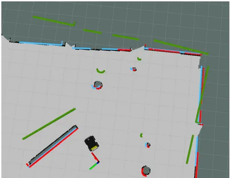
Generally, the term scan denotes in this context a planar laser scanner acting in 2 dimensions, but it can denote any type of laser scan data. A point cloud generally denotes a set of data points in a three-dimensional space; this can be generated from either a two or three-dimensional laser scanner. The purpose of scan matching is to minimize the difference between two point clouds. An example of scan matching being applied can be seen in Figure (1). Here the source scan (green) from the badly localized robot is attempted to be matched with the target scan (red). The target scan is generated by a robot not seen in the image, a few meters down. After applying the transformation retrieved from the scan matching algorithm the transformed scan (teal) can be seen, aligning the transformed scan with the target scan. The main idea in this thesis is that this transformation can be used for localization, ignoring the need for a complicated detection algorithm.
Figure 1: Here the source scan (green) is attempted to be matched with the target scan (red). After applying the transformation retrieved from the scan matching algorithm the transformed scan (teal) can be seen. The axis seen at the bottom represents the transform from the source to the target scan in relation to the current position (the Husky robot).
2.4
Iterative Closest Point - ICP
Iterative Closest Point (ICP) is an algorithm used to solve the scan matching problem, which is how to align two scans to minimize the error between them. The algorithm iteratively minimizes the distance between points starting with an initial guess [13]. The resulting transform between the clouds can be utilized to evaluate the offset between these clouds. A variant to ICP is Point-to-Line Iterative Closest Point (PLICP), A. Censi [13] describes the major difference being that standard ICP uses to-Point metric for matching the points meanwhile the PLICP variant uses a Point-to-Line metric. The PLICP algorithm achieves superior performance over standard ICP unless it receives a large initial displacement error. To overcome this problem, another algorithm was used [14]; this algorithm corrects for the bad initial guess, hence outperforming the standard ICP. 2.4.1 Normal distribution transform - NDT
Normal Distribution Transform (NDT) is a scan registration algorithm that similarly to ICP can be used to align scans. The transform applied to the scan generates a smooth function representation that allows utilizing existing numerical optimization e.g. Newton’s method for scan registration [15]. The original NDT algorithm was implemented in 2D. While most scan matching algorithms such as ICP tries to find correspondences between features, 2D NDT instead divides the problem into a grid where each cell is assigned a normal distribution representing the local probability of measuring a point. With the use of Newton’s algorithm, there is no need for establishing correspondences for the scan match [16].
2.5
Kalman Filter - KF
The Kalman filtering estimator is considered by several to be one of the greatest discoveries in the twentieth century and of statistical estimation theory [17]. The Kalman filter provides reliable state estimation despite noisy measurement. The original Kalman Filter assumes a linear system while several variations have been made to allow for estimating non-linear state transitions. The Kalman Filter consists of two steps, the prediction step, and the correction step. An internal model is used for the state transition that is evaluated in the prediction step, this is thereafter corrected
according to the Kalman gain. The size of the Kalman gain depends on the assumed reliability of the previous state estimate or the assumed reliability of the measurement reading.
2.5.1 Extended Kalman Filter - EKF
The Extended Kalman Filter addresses the problem of utilizing non-linear measurements or a non-linear process instead of the linear system assumed in the standard Kalman Filter. By using the partial derivatives of the process and measurement functions one can compute estimates even when facing non-linear relationships [18].
The EKF is one of the most commonly used tools in the field of robotics for state estimations. As most of the state transitions and measurements are not linear, the original Kalman filter is hardly applicable as the linearity requirements can not be neglected. The Extended Kalman Filter allows for relaxing on this linearity requirement. The EKF utilizes linear Taylor expansion to approximate the non-linear state transition and measurements. The filter is highly computationally efficient, this is because of its belief model being simple multivariate Gaussian distribution. A major drawback of the EKF is how the Taylor approximation treats the Gaussian variables going through the filter, only the mean of the distribution is utilized. A wide Gaussian of the random variable can ruin the function approximation. A way around this is to utilize an Unscented Kalman Filter with sigma points to overcome this issue [10].
2.5.2 Centralized Extended Kalman Filter - cEKF
The Centralized Extended Kalman Filter (cEKF) was utilized by P. Kondaxakis et al. [17,19] on multi-robot localization; this filter treats the multiple robots as a single state. The ”Centralized” in ”cEKF” denotes that it is an EKF that has combined several states into one state transition matrix, several robot states will be represented as a single state matrix.
With the cEKF approach, it was possible to combine landmark observations in a multi-robot scenario to easily pass the relative measurements to the other robots. Three robots could with known landmarks share estimate relative measurements between each other to improve the individ-ual localization. A major motivation for this implementation was to allow multiple robots to move concurrently and be able to model the accumulating error, meanwhile, other localization methods could suffer from an accumulating error or dramatic failures from false-positive detections of other robots. They utilized this cEKF as a map-free localization algorithm that could move unrestricted in unmapped environments. This modular implementation could add and detach robots to the system model, where a high number of robots resulted in increased stability of the system [19].
2.6
Related Work
In a paper by E. Ward et al. [20] the authors focus on how a single motorized vehicle can achieve compare-able results using ICP compared to more complex methods for scan matching. Their proposed solution utilizes Solid State mono pulse short-range radar which they utilize as a cheap alternative to LiDAR, with the added benefit of being able to work in harsh weather and retrieve Doppler based relative velocities.
M. Barczyk et al. [21] utilized a point cloud from a depth camera to improve the pose estimate, two variations to an EKF were used: the Invariant Extended Kalman Filter and the Multiplicative Extended Kalman filter. ICP was utilized to scan match the data relative to the pre-recorded map, they only compared the two variations of the EKF to each other and relative the ground truth.
The paper ”A Monte Carlo algorithm for multi-robot localization” by D. Fox et al. [1] focuses on extending a Monte Carlo algorithm to synchronize the belief states between the robots upon a confirmed visual contact. The authors highlight how repeated integration of the robot’s belief in a short time will result in overconfidence in their positioning, therefore they limit the synchronization to never occur on negative sights (when they can’t see another robot) and use a timer that stops the synchronization to trigger too often. These two limitations were enough to yield significantly improved performance.
A. Martinelli et al. [5] utilized relative bearing and distance measurements between multiple robots and integrated them in an extended Kalman filter to achieve superior performance to dead reckoning alone. This solution does not utilize an algorithm for global positioning from e.g. Monte Carlo localization but instead relies completely on the odometry and the relative poses retrieved from the sensors. The localization improved strongly when utilizing the additional measurements. In a similar fashion by S. Xingxi et al. [22] a distributed unscented Kalman filter is utilized on each local robot. Whenever a robot is lost they will use relative observations towards other robots to improve their localization. They conclude that this is an effective solution even for A heteroge-neous group of robots.
P. Kondaxakis et al. [19] used a setup of three robots that utilize relative measurements between the robots as well as local landmarks to localize. A solution was proposed using a cEKF to improve localization. This reduced the dependence on external landmarks.
R. Dietrich et al. [6] took a completely different approach. They utilized deep learning to detect robots using pre-known shapes, the occupancy grid-map data is feed into a neural network that outputs the position and classification of nearby robots. They utilize solely 2D laser scans to generate this occupancy grid-map. Their solution can function well in fleets of robots localizing in sparse structured areas.
Y. Zhuang et al.[23] developed a method that unlike previous solutions does not utilize a de-tection method for seeing the other robot, instead they utilize the shared sensor data for the surroundings to use in Metric based ICP. This is the most similar work to the planned implemen-tation as it does not use a detection algorithm to find the position of the robot but instead position it using the transform between the scans.
3
Problem formulation
3.1
Hypothesis
Based on the problem formulation, the hypothesis for this thesis is formulated as:
It is possible to improve the localization of an individual robot by utilizing an Extended Kalman Filter with a collaborative scan match with a nearby
stationary robot as measurements.
3.2
Research questions
In an attempt to verify the hypothesis, the following research questions are expressed:
RQ1: What algorithms and configuration can be utilized to obtain relative pose estimates with col-laborative scan matching?
Using the scans from multiple robots, the goal is to develop a practical implementation with suitable scan matching algorithms to improve localization. The output from the scan match-ing algorithm is a transformation, which will be interpreted as a pose of where the robot should have been in relation to the current estimate. This pose adjustment generated from the transformation is referred to as the corrected pose estimate.
RQ2: How can the relative pose estimates extracted from collaborative scan matching be filtered for validity as well as estimating the error in this observation?
After the corrected pose estimate has been retrieved, explore how one should evaluate if this measurement is a valid estimate, and what covariance matrix should be attached to this measurement. If there is no covariance matrix attached to this measurement, it becomes difficult to fuse with other sensor data, this is because the covariance matrix is used to express the estimated error.
RQ3: How can the relative pose estimates extracted from collaborative scan matching be utilized for localization?
After one has generated these pose estimates with an attached error estimate, explore exam-ples of configurations that can utilize this data, followed by evaluation of how these configu-rations perform in comparison to a more standard solution.
3.3
Limitations
Only focus on 2D laser scans, no other type of sensor such as a 3D LiDAR.
No focus on mapping aspects, e.g. Simultaneous Localization And Mapping (SLAM). Will not focus on swarms of robots, just handful at max which can operate independently. Only one robot is active, the other two robots remain stationary and have known initial positions.
Will only operate the robot in three degrees of freedom, in this case, a flat ground.
Assume the environment does not have sparse geometrical data, e.g. area is not a large empty space.
4
Method
The method used for this work is a quantitative iterative process where different solutions are tested and evaluated, then implemented. If an implementation becomes infeasible compared to another solution it can be switched out. The initial plan is set based on several weeks of research in related works. Related work is reread and researched for options if an implementation does not work as intended. The evaluation is quantitative in the sense that it compares the results to a simulated scenario; these values give a sense of the robustness and accuracy of the current implementation. The test cases can be heuristic during development but will be more clearly defined when comparing different solutions in the final stages.
To answer RQ1: two different scan matching algorithms NDT and Generalized Iterative Closest Point (GICP) are implemented, with an initial guess based on the robot’s position according to the map frame. This new pose estimate derived from the transformation calculated from the scan matching algorithms is then evaluated qualitatively relative to the ground truth.
To answer RQ2: the scan matching pose estimate is then further filtered in an attempt to achieve higher accuracy of the pose estimates relative to the ground truth. This is also a qualita-tive evaluation.
To answer RQ3: the pose estimate generated from the scan matching is now fused in an EKF to improve the localization of a simulated robot. Another configuration is also attempted where the Monte Carlo Localization is reset under specific conditions to incorporate the data when the Monte Carlo Localization is deemed unreliable. As the state covariance estimate will grow to infinity over time if no measurements are received, the reset scenario should not trigger unless the covariance estimate shows a low variance for the pose estimate.
5
Implementation
5.1
Scan matching
To help localize the robots relative to each other, one tries to deduce the translation between the robots’ laser scan data. If the scans match perfectly for the same obstacle, then it implies that these robots have the correct distance between each other. This does however not imply that the global localization is perfect. The robots could, in theory, be completely lost in global positioning, but still have a perfect relative position estimate. A transformation is made between the current estimate of the transformation between the main robot and the stationary robots in the proximity. This transformation is made to the laser scans of the robots such that their scans are both in the global coordinate system. This transform becomes the initial guess for the scan matching algorithm. One can expect less error from the scan matching algorithm the closer the robots are, though this requires the current belief state to match this as otherwise, it would result in a bad initial guess. The typical scan matching algorithm ICP has an implicit assumption of full overlap [24], but this is not the case in robots operating with several meters of distance between them. Partially overlapping scans will be much more likely, this is why different algorithms than standard ICP were utilized. The underlying framework for handling the point cloud data as well as estimating the reciprocal correspondences were provided by the Point Cloud Library (PCL).
The outcome from the scan match is evaluated in a second step: there has to be a minimum amount of reciprocal (shared) correspondences between the outcome and the target transformation. In this implementation, 200 which is roughly 25% of the rays from the scan are needed to be reciprocal correspondences between the output and target scan. This correspondence detection is done using a k-d tree search to find the closest neighbor of the points in the outcome and target cloud. An additional parameter for the ”extra” filtered is to set a low max distance for the correspondences in the final step as well. These should together only allow for scan matches that have both significant overlaps and have enough ”points” to conclude that it is a valid match. This implementation goes under the assumption that one wishes to only pass on accurate pose estimates and be careful with publishing unsure measurements. A robust solution should be able to function stand-alone without the collaborative scan matching. The idea behind this heuristic solution is, that only specific segments should be required to have a good overlap. Although it is a very simple model that does not try to make sure specific planes are aligned properly, the early testing does seem to validate this concept by removing outliers. If the robots have sparse geometrical information, the number of ”points” threshold should enforce there is enough geometrical information to provide a valid transform between the robots. Finally, the covariance matrix is estimated using the method developed by P. Sai Manoj et al. [25], although a set amount of extra variance is added to avoid jitter when fusing it with the EKF. Note that although the method for evaluating the covariance error is created for 3D, it is used for practical reasons, where the laser scan is converted into a flat 3D point cloud internally for compatibility with the point cloud library that supplies the algorithms used in this thesis.
The scan implementation used was developed by K. Koide [26]; he created a package contain-ing multi-threaded and optimized versions of NDT and GICP. K. Koide originally utilized this implementation in the paper [27] for scan matching in a SLAM framework. In this framework, one combined the scan matching transform with an angular velocity sensor inside an unscented Kalman filter.
5.2
Extended Kalman Filter implementation
For the thesis work, the robot localization package was used due to its accessibility and ease of use. Previously, a more complex cEKF model was proposed, but problems with accuracy in early tests and time constraints caused a switch to the existing robot localization package. As the measurement model for this filter has been handed to the sender of the sensor data, it relies on them publishing a reasonable covariance. This is especially bothersome when fusing multiple positions as one pose publisher with a covariance matrix containing low variances. A low covariance pose would almost erase any effect of any other pose being published, in parallel with a decimal larger variance. To avoid jitter when using the pose estimates generated by the scan matching node, the covariance matrix is padded with additional variance (the diagonal of the matrix) to give it
a slower convergence. A solution to having multiple poses deciding the position, is to allow only the most reliable pose to decide the position; then integrating the change in the other less reliable poses to estimate the velocities instead. This was deemed highly inaccurate in early tests, likely due to the relatively low frequency of the scan matching node.
5.3
Adaptive Monte Carlo Localization implementation
The implementation for AMCL is based on the existing ROS package created by Brian P. Gerkey et al. [28]. This implementation is based on the KLD sampling version proposed by Dieter Fox [10]. This implementation uses the same tuning for AMCL as the original Clearpath Husky robot [9]. The pose published by AMCL contains a covariance matrix that is used in the AMCL reset configuration to determine when the robot is lost. Upon resetting AMCL one publishes a pose in combination with a covariance matrix. This will reinitialize the particles around the provided pose with a spread based on this provided covariance matrix. This pose with covariance will be used for re-initializing the particles, a high variance in the covariance matrix will result in a larger spread of the particles.
5.4
Simulation
To evaluate the results, the simulation environment Gazebo is used to generate sensor data and ground truth data. A pre-mapped area is used to allow for AMCL to localize within. A 2D LiDAR, an Inertial Measurement Unit (IMU) is simulated with added Gaussian noise. The wheel encoder does not have any explicitly added noise and is generated by the standard diff drive controller from the ros controllers stack. The simulation is based on the Clearpath Robotics Husky implementation [9], although a heavily edited version, that among other changes, contains multiple Husky robots under different namespaces.
5.5
Evaluation metric
The metric used for evaluating the localization is Absolute Pose Error (APE). The APE is based on the absolute relative pose between estimated pose and the reference pose obtained from the ground truth. A software previously developed by M. Grupp [29] is used to evaluate the recorded pose estimates using the following metrics:
Ei= Pest,i Pref,i= Pref,i−1 Pest,i∈ SE(3) is the inverse compositional operator, which calculates the relative pose.
(Translation error) AP Ei= ktrans(Ei)k
(Rotation error) AP Ei= |(angle(logSO(3)(rot(Ei)))|
logSO(3)(·) is the inverse of expso(3)(·) (Rodrigues’ formula)
Thereafter, median, mean, root mean square error, maximum and minimum error values are calculated. Root mean square error (RMSE) is calculated using the following:
RMSE = v u u t 1 N N X i=1 AP E2 i
6
Experimental setup
To evaluate the implementation a simulation environment is used to record the sensor data as well as the ground truth. Different configurations for the localization are then used with this recorded data.
6.1
Gazebo Simulation setup
In the Gazebo simulation environment, three robots are equipped with 270◦ 2D laser scanners, as well as wheel encoders and IMU. The three robots are initialized in three different locations relative to the map frame, (0,0), (-3,0) and (-5,0) relative to the maps X-Y frame. The first robot initialized as the origin (0,0) then drives around the area clockwise while suffering minor obstruction from an obstacle between this robot and the other two. The robot later reverses backward into a barrier to simulate collision and slippage. After a short reverse, the robot drives forward towards the initial starting position in the origin. Two props in the form of two dumpsters were added next to the middle barrier seen in Figure (2) to simulate a less ideal scenario for the global positioning estimate from AMCL, as these props are not on the pre-recorded map. The IMU sensors have a predefined drift and noise of 0.05 standard deviations for the orientation, angular velocity, and linear accelerations. The purpose of the less than ideal environment for the typically used AMCL algorithm configuration with IMU with wheel encoders is to have a scenario where AMCL does not provide highly reliable data. A better environment for AMCL would result in a better initial guess for the scan matching methods and would make it difficult to adjust for significant errors.
Figure 2: Visual representation of the playpen environment in the Gazebo simulation.
6.2
Test case configurations
Several layouts for the localization setups were applied to the sensor data recorded in the simulation step. In all layouts, the EKF fuses the Wheel encoder as an X-axis velocity and Y-axis velocity, meanwhile, the IMU is fused as rotation around the Z-axis and angular velocity around the Z-axis.
6.3
Scan match configurations
The output from the multi-robot scan matching node utilizes either GICP or NDT. First, the scan matching node is evaluated qualitatively, based on the Wheel encoder and IMU with AMCL scenario as an initial guess for the scan match transformation. It displays the scan match between main robots scan to the second robot, which is stationary at the position -3.0 in the X-axis, and 0.0 in the Y-axis, relative to the map frame. The purpose is to evaluate the corrected pose estimate before it is being used as feedback to the localization. The quantitative testing is done with both scan matching algorithms; having a high enough number of reciprocal correspondences was the main metric for filtering. As the maximum distance for correspondences was set to 3 meters, it likely never failed due to the maximum distance condition, but rather to the number of correspondences. Having the stricter filtering would have likely resulted in too low frequency for the EKF to be able to use the collaborative position estimates properly, which is why only the number of correspondences was used for the test cases.
6.3.1 Wheel encoder and IMU with AMCL
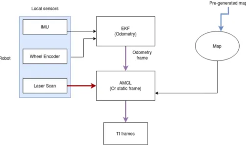
This is a standard configuration where the odometry is estimated using an EKF that fuses linear velocities from the wheel encoder with the angle and angular velocity from the internal IMU. AMCL with the help of a pre-recorded map corrects from the drift accumulated by the EKF, see Figure (3) for the layout.
Figure 3: Brief description of the setup of the ”Wheel encoder and IMU with AMCL” layout.
6.3.2 Wheel encoder and IMU with AMCL that uses scan match reinitialization This scenario uses the GICP scan match averaged using an additional EKF. It was chosen to only display the GICP outcome, as the NDT scenario had similar but worse results. It was deemed redundant to use both algorithms as it is non-deterministic when AMCL falls below the specific threshold required for the reinitialization to trigger, thus comparing the two algorithms became unreliable.
6.3.3 Collaborative scan match fused with wheel encoder and IMU
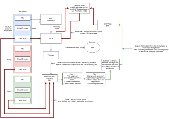
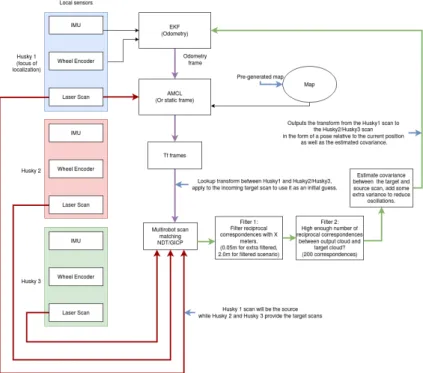
This configuration is evaluated using a collaborative scan match based on the scan matcher utilizing either NDT or GICP for the position estimate in the EKF state estimation, while the wheel encoder and IMU are identically in the filter as in the ”Wheel encoder and IMU with AMCL” scenario. See Figure (3 for the description of the layout. This layout has a static frame for the map to odometry frame instead of using AMCL to correct the drift.
Figure 4: Brief description of the setup of the ”Wheel encoder and IMU with AMCL that uses scan match reinitialization” layout.
6.3.4 Collaborative scan match fused with wheel encoder and IMU with AMCL Same as the ”Collaborative scan match fused with wheel encoder and IMU” except AMCL controls the map to odometry frame, thus trying to localize itself and offset the drift generated.
Figure 5: Brief description of the setup of the ”Collaborative scan match fused with wheel encoder and IMU with/without AMCL” layout.
7
Results
The following section presents the results from the pose estimates generated by the localization configurations as well as the scan matching algorithms. Note that all sensor and ground truth data has been generated from the simulation environment, the interpretation of this data is left to the individual test configurations. The scan matching outputs, AMCL pose estimate, and the EKF outputs are not pre-recorded for each test case, only the sensor data is pre-determined for each run. See the evaluation metric section for an explanation of Absolute Pose Error (APE).
7.1
The scan matching algorithms and the filtering results
In this section the accuracy of the scan matching algorithms are evaluated, this scenario is a non-feedback based case where the initial guess is from the scan matching independent localization. This localization consists of the wheel encoder and IMU fused in an EKF for the odometry used by AMCL, see the implementation section for more details. The ground truth is presented which is generated by the simulation environment. In the figures below, the errors of the pose estimates generated from the scan matching algorithms GICP and NDT are presented. The errors of these pose estimates are separated into the X-axis and the Y-axis for easy visualization, but the rotation errors are not presented in this section. In Figure (6,7) the X-axis and Y-axis errors are plotted without any post-filtering.
Figure 6: The initial scan matching X-position estimate from the scan matching nodes.
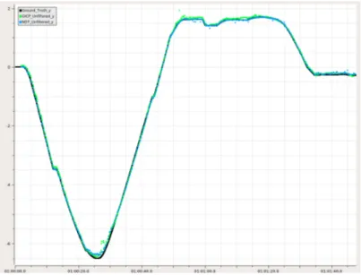
Figure 7: The initial scan matching Y-position estimate from the scan matching nodes. Below in Figure (8,9), the output scan generated by the scan matching algorithm has been filtered based on the correspondence to the target scan. If there is a large number of shared correspondences between these scans one will allow it to pass the filter and a pose estimate is published. This type of filtering is used in the upcoming sections where scan matching is combined with the different localization configurations.
Figure 8: The scan matching pose X-position estimated with filtering based on the number of correspondences. The estimated odometry pose is the AMCL output based on the wheel encoder and IMU scenario; this is independent of the scan matching outputs (does not receive feedback from the scan match).
Figure 9: The scan matching pose Y-position estimated with filtering based on the number of correspondences. The estimated odometry pose is the AMCL output based on the wheel encoder and IMU scenario; this is independent of the scan matching outputs (does not receive feedback from the scan match).
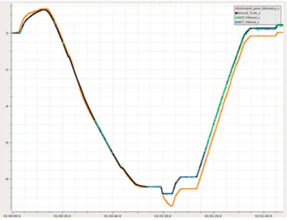
Below in Figure (10,11), scan generated by the scan matching algorithm has been filtered based on the correspondence to the target scan. The difference from the above results is that the maximum distance for searching for these correspondences is only 0.05 meters. This is very low compared to the above example where it has a 2.0 meters search radius for these correspondences. In these figures the odometry estimate is now visualized as well for a final comparison; this is the initial guess used for the scan matching.
Figure 10: The scan matching pose X-position estimated with filtering based on the number of correspondences as well as strict filtering based on the distance for the correspondences. The estimated odometry pose is the AMCL output based on the wheel encoder and IMU scenario; this is independent of the scan matching outputs (does not receive feedback from the scan match).
Figure 11: The scan matching pose Y-position estimated with filtering based on the number of correspondences as well as strict filtering based on the distance for the correspondences. Estimated the odometry pose which is based on wheel encoder and IMU with AMCL; this is independent of the scan matching outputs (does not receive feedback from the scan match).
7.2
Map visualization of the scan matching algorithms and the filtering
Below in Figure (12) the unfiltered pose estimate generated with the scan matching algorithms NDT and GICP is visualized, this is the same data as seen in Figure (8,9). The ground truth generated from the simulation is visualized in addition to the pose estimates generated by the scan matching algorithm.
Figure 12: The scan matching pose estimate, unfiltered. The estimated odometry pose is the AMCL output based on the wheel encoder and IMU scenario; this is independent from the scan matching outputs (does not receive feedback from the scan match).
Below in Figure (13), the scan generated by the scan matching algorithm has been filtered based on the correspondence to the target scan. This is the same data as seen in Figure (8,9).
Figure 13: The scan matching pose estimated with filtering based on the number of correspon-dences. The estimated odometry pose is the AMCL output based on the wheel encoder and IMU scenario; this is independent of the scan matching outputs (does not receive feedback from the scan match).
In Figure (14) the scan matching algorithm transform has been filtered in relation to the target scan and the output scan from the scan matching algorithm, the maximum distance for searching for these correspondences is only 0.05 meters compared to the 2.0 meters used above in Figure (13). This is the same data as seen in Figure (10,11).
Figure 14: The scan matching pose estimated with filtering based on the number of correspondences as well as strict filtering based on the distance for the correspondences. The estimated odometry pose is the AMCL output based on the wheel encoder and IMU scenario; this is independent of the scan matching outputs (does not receive feedback from the scan match).
7.3
Results from the localization configurations
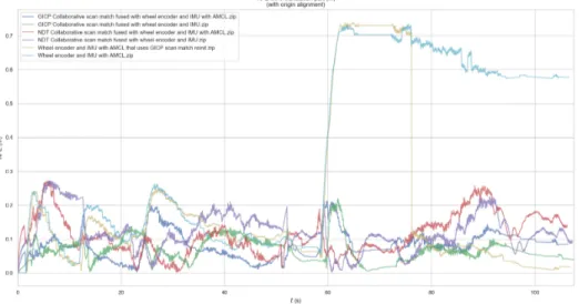
In the following section, the results from the different localization configurations are presented. In Figure (15) absolute pose error related to translation is shown in relation to time, where a small value represents a small error between the ground truth and the current pose estimate. In Figure (16) the statistics of the APE related to translation is presented in a bar plot. The unit for the translation error is in meters.
Figure 16: The resulting Absolute Pose Errors (APE) related to the translation. At time 58 the wheels began slipping causing the drift certain configurations.
Similarly to above the results from the different localization configurations are presented. In Figure (17) absolute pose error related to rotation is shown in relation to time, where a small value represents a small error between the ground truth and the current pose estimate. In Figure (18) the statistics of the APE related to rotation is presented in a bar plot. The unit for the rotation error is in degrees.
Figure 18: The resulting Absolute Pose Errors (APE) related to the rotation.
7.4
Absolute pose error statistics from the localization configurations
In the following section the APE statistics seen in Figure (16,18) are presented in tabular form. The translation error is based on the pose estimate versus the ground truth, the same applies for the rotation error but this is solely based on the rotation. The translation error is in meters while the rotation error is in degrees.
Absolute Pose Translation Error Statistics (in meters)
Localization method max mean median min rmse sse std
GICP Collaborative scan match fused with wheel encoder and IMU with AMCL 0.21 0.08 0.08 5.55e-18 0.09 23.42 0.04 GICP Collaborative scan match fused with wheel encoder and IMU 0.22 0.07 0.06 3.39e-21 0.08 16.81 0.04 NDT Collaborative scan match fused with wheel encoder and IMU with AMCL 0.27 0.11 0.10 0.00 0.13 44.26 0.06 NDT Collaborative scan match fused with wheel encoder and IMU 0.27 0.12 0.11 2.71e-20 0.13 50.25 0.06 Wheel encoder and IMU with AMCL that uses GICP scan match reinit 0.74 0.19 0.11 4.91e-18 0.30 250.16 0.23 Wheel encoder and IMU with AMCL 0.73 0.35 0.21 5.55e-18 0.44 539.47 0.26 Table 1: Table displaying the statistics of the translation error from the different localization configurations.
Absolute Pose Rotation Error Statistics (in degrees)
Localization method max mean median min rmse sse std
GICP Collaborative scan match fused with wheel encoder and IMU with AMCL 4.95 0.61 0.48 2.06e-17 0.88 2198.38 0.64 GICP Collaborative scan match fused with wheel encoder and IMU 4.76 0.60 0.35 2.88e-18 0.97 2699.59 0.76 NDT Collaborative scan match fused with wheel encoder and IMU with AMCL 9.12 0.94 0.55 3.06e-17 1.54 6673.00 1.22 NDT Collaborative scan match fused with wheel encoder and IMU 9.22 1.24 0.75 5.02e-18 1.91 10379.46 1.45 Wheel encoder and IMU with AMCL that uses GICP scan match reinit 3.61 1.11 1.09 1.59e-18 1.21 4197.43 0.50 Wheel encoder and IMU with AMCL 4.43 1.46 1.04 4.38e-18 1.82 9345.81 1.08 Table 2: Table displaying the statistics of the rotation error from the different localization config-urations.
7.5
Absolute pose error from the localization configurations mapped
relative to trajectory
To further allow the evaluation of the different localization configurations, the pose estimates are visualized as a trajectory separately for each configuration. The figures below present the paths used for calculating the statistics seen in Table (1,2), see also Figure (16,18). Note that the two robots used for assisting localization are not shown in the figures, they are at the positions (-3,0) and (-5,0) facing positive x-direction, the initial position for the moving robot is at (0,0) facing positive x-direction then travels clock-wise. The reference line shown is the ground truth of the
position, this is generated from the simulation environment. The colored line is the estimated path with the color describing the translation aspect of the APE relative to ground truth, see the evaluation metric section for an explanation of Absolute Pose Error (APE).
Here in Figure (19) is the localization estimate of the configuration that utilized an EKF to fuse the pose estimates from the GICP algorithm with IMU and wheel encoder. This output from the EKF is used as a guess for the localization algorithm, AMCL. The output of AMCL is then used as an initial guess for the scan matching algorithm in relation to the map.
Figure 19: The Absolute Pose Error related to translation, for the ”GICP Collaborative scan match fused with wheel encoder and IMU with AMCL” scenario.
Here in Figure (20) is the localization estimate of the configuration that utilized an EKF to fuse the pose estimates from the GICP algorithm with IMU and wheel encoder. This output is not fused into AMCL unlike the above example. This had overall the least error in regards to translation.
Figure 20: The Absolute Pose Error related to translation, for the ”GICP Collaborative scan match fused with wheel encoder and IMU” scenario.
In Figure (21) is the localization estimate of the configuration that utilized an EKF to fuse the pose estimates from the NDT algorithm with IMU and wheel encoder, this odometry is then used as a guess for the localization algorithm AMCL. The only difference to configuration seen in Figure (19) is that the scan matching algorithm NDT is used instead of GICP.
Figure 21: The Absolute Pose Error related to translation, for the ”NDT Collaborative scan match fused with wheel encoder and IMU with AMCL” scenario.
In Figure (22) one can see the results of the NDT variation of the EKF fusing wheel encoder, IMU and NDT pose estimates. The setup is similar to the GICP version seen in Figure (20
Figure 22: The Absolute Pose Error related to translation, for the ”NDT Collaborative scan match fused with wheel encoder and IMU” scenario.
In Figure (23) one can see the scan matching free variation, simply fusing wheel encoder and IMU, this odometry is then used as a guess for the localization algorithm AMCL. This is the same configuration used for evaluating the scan matching algorithms seen in Figure (13). Note how the wheel slippage at the top left causes a significant error.
Figure 23: The Absolute Pose Error related to translation, for the ”Wheel encoder and IMU with AMCL” scenario.
The following configuration is almost identical to the one seen in Figure (23), it uses an EKF that fuses IMU and wheel encoder for an initial guess for AMCL. The difference here is that when AMCL publishes a high covariance in its pose estimate it will reset with a scan matching generated pose estimate. This pose estimate is generated with the GICP algorithm which is fused in an EKF. In Figure (24) one can see the results from this configuration. The reset of the particle filter is triggered at roughly the (-6.2,1.8) position, the translation error drops significantly after this reset.
Figure 24: The Absolute Pose Error related to translation, for the ”Wheel encoder and IMU with AMCL that uses GICP scan match reinitialization” scenario.
8
Conclusion
8.1
Scan matching method
Overall, NDT gave more accurate results but with the current settings, GICP had a significantly higher frequency, seen in the unfiltered Figure (6,7). The extra steps of filtering resulted in highly accurate results, but could result in data being sparse, see Figure (10,11) for the extra filtered results. For the following sections the data is filtered with the same settings seen in Figure (8,9), which has a very high maximum distance allowed for the reciprocal correspondences.
8.2
Wheel encoder and IMU with AMCL
This standard configuration performed the worst overall, likely due to a bad estimate of wheel odometry, as well as AMCL not performing optimally with the extra two props in the proximity. See Figure (23).
8.3
Scan matching fused with wheel encoder and IMU
The scan matching algorithms GICP and NDT were used in this configuration. This version improved significantly over the ”Wheel encoder and IMU with AMCL” configuration. See Figure (20,22).
8.4
Scan matching fused with wheel encoder and IMU with AMCL
The scan matching algorithms GICP and NDT were used in this configuration. Here one of the main problems with this approach becomes visible; the incompatibility with AMCL. In some cases, when the Monte Carlo Localization tries to correct for any error by adjusting the odometry frame, it will get counteracted by the scan matching pose estimate. See the translation error in Figure (19,21). The scan matching poses and AMCL can create a feedback loop where they try to correct for the error in each other, this is less obvious with the high amount of variance padding on the scan matching output. The AMCL node also gets somewhat fooled by the odometry created with the scan match. Even if the robot is stationary, it can trigger the ”minimal motion” parameters in AMCL causing it to update even when no real motion has occurred, due to the scan matching poses moving the odometry frame to a more correct position. However, AMCL is unable to differentiate this from real motion in the current implementation.
8.5
Global positioning
This configuration resets AMCL using a filtered pose estimate extracted from GICP, the NDT version was excluded it was deemed redundant due to the worse performance. The current im-plementation of reinitializing AMCL with the external filter works somewhat to adjust for the accumulated error. As seen in Figure (15) a major drop in the translation error occurs at roughly time 75. Although it worked in this case, basing the trigger condition of the covariance matrix from AMCL was not robust. As the covariance output from the AMCL package is based on the spread of the particle clusters, it would likely have worked better with a global positioning algorithm that tries to solve this internally. The reset should be considered a risky approach as one loses the data AMCL has accumulated right before and after the reset.
8.6
Summary
The hypothesis proved to be feasible within the testing environment, as the localization is im-proved with the collaborative scan matching utilized by an EKF, even in multiple layouts. The scan matching between the robots is shown to provide accurate information that could improve the odometry or global positioning, see Figure (16,18) for the comparison graphs. The GICP im-plementation was more accurate than the NDT imim-plementation when fused with the EKF. The EKF fusion method works well stand-alone but is not efficiently combined with the currently im-plemented Adaptive Monte Carlo Localization algorithm. The reinitialization method can correct
major faults but the current heuristic method of judging the accuracy based on the cluster covari-ance appears unpredictable. Several problems remain to be solved, such as having multiple robots using the scan for the localization without suffering from feedback loops. All three search questions are answered. For the first research question: the NDT and GICP configurations allow for estimat-ing the relative pose estimate. For the second research question: the filterestimat-ing based on reciprocal correspondences with and without low maximum search distance could filter out the worst outliers. For the third research question: the EKF is effective at fusing the data for an accurate estimate, but is conflicting or hard to apply on the used map-based localization algorithm.
9
Discussion
In regard to Research Question 1:
The current layout of applying NDT and GICP to generate a pose estimate was quite effective in this specific circumstance.
In future work, one could use sensors such as the IMU and wheel encoders in the scan matching prediction to improve the accuracy. The current method risks having a slightly delayed estimate as it will use slightly outdated data.
In this testing environment, only one robot was mobile, while the other robots were stationary with a known position. The collaborative scan matching measurement acts on the assumption that the stationary robot does have a correct pose relative to the world. Therefore, a more dedi-cated solution that considers this error as well as providing an estimate of it, would likely utilize the collaborative scan matching more efficiently. Currently, the implementation applies an extra variance to the covariance matrix to reduce the jitter when combined with an Extended Kalman Filter, which seems to give a bias towards the GICP algorithm that operates at a higher frequency than the NDT algorithm.
One could have improved the performance with an improved initial guess by using e.g. feature descriptors such as the SHOT descriptor [25,30].
In regard to Research Question 2:
The filtering method of validating based on a threshold of reciprocal correspondences was quite effective as it could remove the worst outliers. Applying a limited maximum distance for the correspondences could guarantee highly accurate estimates. One drawback, however, is the low frequency of the highly filtered pose estimates. More tuning and more filtering could have been done in the scan matching algorithms to have fewer estimates being filtered way. The filtering based on the number of correspondences was only evaluated using reciprocal correspondences;w one could likely have used a non-reciprocal correspondences estimation method. How this filtering method will behave on lasers with different specifications was not evaluated, e.g. how would this behave with a low-density laser scan matched with a high-density laser scan. One would likely have to hand tune specific thresholds for different laser configurations or perhaps use a percentage of the points of the sparsest cloud.
In regard to Research Question 3:
On the topic of global positioning, the original goal was to fuse the AMCL output in a filter along with the collaborative scan matches. This proved to be difficult as the AMCL provides a covariance matrix that does not fuse effectively in the filter as it states too optimistic variances.
A global or a completely new fork of it that is more to this type of input, as it currently relies on either one resetting it with the new estimate, or by one improving the odometry. If it was possible to insert a particle or cluster into the AMCL algorithm based on the relative observation, then this data would likely be a lot more efficient to use the collaborative scan. Using the existing multi-robot Monte Carlo Solutions formulated previously by Dieter Fox e.t al[1], with the current pose estimation method, could give significant improvements to existing global positioning sensors without having to reuse the existing sensors. This could hopefully prevent a ”tug-of-war” effect from happening where the AMCL algorithm will conflict with the scan matched pose estimate, as well as the scan matched pose estimate introducing an error from a robot that is badly localized.
One problem that also has to be resolved is when handling large delays in obtaining the initial transformation between the robots. The initial transformation is used as the initial guess for the scan matching method. The possibility to utilize an old estimate to correct the current estimate could be another topic for future work. This topic might however fall under existing SLAM ap-proaches, such as loop closure on previously recorded data in mapping scenarios, as scan matching algorithms have also been already in those scenarios [31]. The current method in this thesis could from one view be very short term mapping which is then applied to nearby robots, although, this current implementation can be applied for high accuracy positioning and recognition of nearby
robots. Previous approaches with neural networks could classify robots based on the shape of the robot [6]. Instead, one could avoid having to train a network for detecting the robot itself , but rather use scan matching with similar sensors to detect its position in the proximity with high precision.
References
[1] D. Fox, W. Burgard, and S. Thrun, “A monte carlo algorithm for multi-robot localization,” 09 1999.
[2] P. Beinschob and C. Reinke, “Graph slam based mapping for agv localization in large-scale warehouses,” in 2015 IEEE International Conference on Intelligent Computer Communication and Processing (ICCP), Sep. 2015, pp. 245–248.
[3] B. Zhang, J. Liu, and H. Chen, “Amcl based map fusion for multi-robot slam with het-erogenous sensors,” in 2013 IEEE International Conference on Information and Automation (ICIA), Aug 2013, pp. 822–827.
[4] S. Panzieri, F. Pascucci, and R. Setola, “Multirobot localisation using interlaced extended kalman filter,” in 2006 IEEE/RSJ International Conference on Intelligent Robots and Systems, Oct 2006, pp. 2816–2821.
[5] A. Martinelli, F. Pont, and R. Siegwart, “Multi-robot localization using relative observations,” in Proceedings of the 2005 IEEE International Conference on Robotics and Automation, April 2005, pp. 2797–2802.
[6] R. Dietrich and S. D¨orr, “Deep learning-based mutual detection and collaborative localiza-tion for mobile robot fleets using solely 2d lidar sensors,” in 2019 IEEE/RSJ Internalocaliza-tional Conference on Intelligent Robots and Systems (IROS), Nov 2019, pp. 6706–6713.
[7] M. Quigley, K. Conley, B. Gerkey, J. Faust, T. Foote, J. Leibs, R. Wheeler, and A. Y. Ng, “Ros: an open-source robot operating system,” in ICRA workshop on open source software, vol. 3, no. 3.2. Kobe, Japan, 2009, p. 5.
[8] B. G. VaughanAndrewHoward, “Theplayer/stageproject: Toolsformulti-robotand distributed sensor systems,” InProceedings of the International Conference on Advanced Robotics (ICAR 2003)pages 317-323, Coimbra, Portugal, June 30 - July 3, 2003., 2003.
[9] Clearpath Robotics, “Clearpath Husky,” [Online]. Available: https://github.com/husky/ huskyAccessed: 2020-04-10.
[10] S. Thrun, W. Burgard, and D. Fox, Probabilistic Robotics (Intelligent Robotics and Au-tonomous Agents). The MIT Press, 2005.
[11] F. Dellaert, D. Fox, W. Burgard, and S. Thrun, “Monte carlo localization for mobile robots,” in Proceedings 1999 IEEE International Conference on Robotics and Automation (Cat. No.99CH36288C), vol. 2, May 1999, pp. 1322–1328 vol.2.
[12] D. Fox, “Kld-sampling: Adaptive particle filters and mobile robot localization,” Advances in Neural Information Processing Systems (NIPS), 2002.
[13] A. Censi, “An icp variant using a point-to-line metric,” in 2008 IEEE International Conference on Robotics and Automation, May 2008, pp. 19–25.
[14] A. Censi, “Scan matching in a probabilistic framework,” vol. 2006, 06 2006, pp. 2291 – 2296. [15] M. Magnusson, “The three-dimensional normal-distributions transform — an efficient repre-sentation for registration, surface analysis, and loop detection,” Ph.D. dissertation, 12 2009. [16] P. Biber and W. Straßer, “The normal distributions transform: A new approach to laser scan
matching,” in Proceedings 2003 IEEE/RSJ International Conference on Intelligent Robots and Systems (IROS 2003)(Cat. No. 03CH37453), vol. 3. IEEE, 2003, pp. 2743–2748.
[17] P. Kondaxakis, A Modular Framework for Multi-robot Localization Scenarios: Developing and Distributing Localization Algorithms Utilizing Kalman Filter Estimators, for Mobile Multi-robot Systems. LAMBERT Academic Publishing, 2010.
[18] G. Welch, G. Bishop et al., “An introduction to the kalman filter.”
[19] P. Kondaxakis, V. F. Ruiz, and W. S. Harwin, “Compensation of observability problem in a multi-robot localization scenario using cekf,” in 2004 IEEE/RSJ International Conference on Intelligent Robots and Systems (IROS) (IEEE Cat. No.04CH37566), vol. 2, Sep. 2004, pp. 1762–1767 vol.2.
[20] E. Ward and J. Folkesson, “Vehicle localization with low cost radar sensors,” in 2016 IEEE Intelligent Vehicles Symposium (IV), June 2016, pp. 864–870.
[21] M. Barczyk, S. Bonnabel, J. Deschaud, and F. Goulette, “Invariant EKF design for scan matching-aided localization,” CoRR, vol. abs/1503.01407, 2015. [Online]. Available:
http://arxiv.org/abs/1503.01407
[22] Shi Xingxi, Huang Bo, Wang Tiesheng, and Zhao Chunxia, “Cooperative multi-robot local-ization based on distributed ukf,” in 2010 3rd International Conference on Computer Science and Information Technology, vol. 6, July 2010, pp. 590–593.
[23] Y. Zhuang, Z. Wang, H. Yu, W. Wang, and S. Lauria, “A robust extended h∞ filtering approach to multi-robot cooperative localization in dynamic indoor environments,” Control Engineering Practice, vol. 21, no. 7, pp. 953 – 961, 2013. [Online]. Available:
http://www.sciencedirect.com/science/article/pii/S0967066113000245
[24] A. Segal, D. Haehnel, and S. Thrun, “Generalized-icp.” in Robotics: science and systems, vol. 2, no. 4. Seattle, WA, 2009, p. 435.
[25] S. Prakhya, L. Bingbing, Y. Rui, and W. Lin, “A closed-form estimate of 3d icp covariance,” in Machine Vision Applications (MVA), 2015 14th IAPR International Conference on, May 2015, pp. 526–529.
[26] Koide, Kenji, “NDT/GICP OMP,” [Online]. Available: https://github.com/husky/husky Ac-cessed: 2020-04-10.
[27] K. Koide, “A portable 3d lidar-based system for long-term and wide-area people behavior measurement,” 02 2019.
[28] Brian P. Gerkey, “amcl,” [Online]. Available: http://wiki.ros.org/amclAccessed: 2020-04-10. [29] M. Grupp, “evo: Python package for the evaluation of odometry and slam.”https://github.
com/MichaelGrupp/evo, 2017.
[30] S. Salti, F. Tombari, and L. D. Stefano], “Shot: Unique signatures of histograms for surface and texture description,” Computer Vision and Image Understanding, vol. 125, pp. 251 – 264, 2014. [Online]. Available: http://www.sciencedirect.com/science/article/pii/S1077314214000988
[31] M. Magnusson, H. Andreasson, A. Nuchter, and A. Lilienthal, “Appearance-based loop de-tection from 3d laser data using the normal distributions transform,” 05 2009, pp. 23 – 28.